Radio continuum and CO emission in star-forming galaxies.

We combine the radio continuum images from the NRAO VLA Sky Survey with the CO-line observations from the extragalactic CO survey of the Five College Radio Astronomy Observatory to study the relationship between molecular gas and the star formation rate within the disks of 180 spiral galaxies at 45″ resolution. We find a tight correlation between these quantities. On average, the ratio between the radio continuum and the CO emission is constant, within a factor of 3, both inside the same galaxy and from galaxy to galaxy. The mean star formation efficiency deduced from the radio continuum corresponds to convert 3.5% of the available molecular gas into stars on a time scale of $10^{8}$ yr and depends weakly on general galaxy properties, such as Hubble type or nuclear activity. A comparison is made with another similar analysis performed using the H_α luminosity as star formation indicator. The overall agreement we find between the two studies reinforces the use of the radio luminosity as star formation rate indicator not only on global but also on local scales.

1 Introduction

One of the major goals of the studies of external galaxies is understanding the relationship between the star formation rate (SFR) and the physical condition in the interstellar medium. Several indicators have been suggested to estimate the SFR (of massive stars) in galaxies. These include the U-band magnitude, the strength of Balmer lines emission, the far-infrared (FIR) emission and the radio luminosity; the rates inferred from the different indicators span almost four orders of magnitude going from $10^{-2}$ to $10^{2}$ M${}_{\odot}\leavevmode\nobreak\$yr^-1. Cram et al. (1998) checked the consistency between the SFR deduced from the U-band, H_α, FIR and radio luminosity using a sample of 700 local galaxies. They noted that there are systematic differences between these various indicators. In particular they suggested that the H_α luminosity may underestimate the SFR by approximately an order of magnitude when the SFR is $\geq 20$ M${}_{\odot}\leavevmode\nobreak\$yr^-1. They concluded that the radio continuum luminosity at decimeter wavelengths of a star forming galaxy provides a better way to estimate the current rate of star formation. The radio continuum emission at 1.4 GHz from a star-forming galaxy is mainly synchrotron radiation produced from relativistic electrons accelerated by supernovae explosions (Lequeux 1971). Indeed the radio continuum luminosity appears to be directly proportional to the rate of formation of supernovae (Condon 1992). This view is reinforced by the tight correlation existing between the radio luminosity and the FIR for spiral galaxies (see e.g. Condon 1992). Since the radio continuum at 1.4 GHz does not suffer significant extinction, the radio luminosity constitutes a very useful tool to determine the current SFR in a spiral galaxy.

Since the discovery that stars form in molecular clouds, it is essential to determine, not only the rate, but also the efficiency of conversion of the interstellar gas in stars; i.e. the star formation efficiency (SFE). The SFE measures the formation rate of young stars per unit of mass of gas available to form those stars. Determining the SFE is important to distinguish a situation in which a high SFR indicates a higher efficiency in converting gas in stars rather than a higher gas quantity.

The CO molecule luminosity and the virial mass of giant molecular clouds correlate very well in our Galaxy and in other nearby spirals (Young & Scoville 1991 and references therein). The comparison of different SFR tracers with the mass of molecular clouds provides indeed an important tool to investigate the behaviour of the SFE within and among galaxies. Many studies have been concerned with the behaviour of the star formation process on global scales, averaged over the entire star-forming disk. These works showed that the disk-averaged star formation process is well described by a Schmidt (1959) law of the type $\Sigma_{\rm SFR}\propto\Sigma_{\rm gas}^{N}$, where $\Sigma_{\rm SFR}$ and $\Sigma_{\rm gas}$ are the observable surface density of SFR and total (atomic + molecular) gas density, respectively, and the exponent $N$ typically ranges from 1.3 to 1.5 (Kennicutt 1998).

An interesting development of these global studies, the investigation of the behaviour of the SFE within the disks of the individual galaxies, provides much physical insight into the star formation process itself. The extragalactic CO survey of the Five College Radio Astronomy Observatory (Young et al. 1995, hereafter FCRAO CO Survey) provided a uniform database of CO data for 300 galaxies at a resolution of 45″, opening the possibility to extend the study of the Schmidt relationship of the SFR versus the H₂ density over the same physical regions well inside the galaxy disks. Since the star formation process involves the molecular gas directly, some authors recognized that the determination of the Schmidt law assumes a clear physical meaning if restricted to this gas component. Moreover, in the considered regions the molecular gas is dominant over the atomic one and, contrary to this latter, its azimuthally averaged distribution follows closely the radial profiles of the main SFR indicators (Tacconi and Young 1986, Young & Scoville 1991). Rownd & Young (1999; hereafter RY99) conducted an H_α imaging of 121 of these galaxies, determining the local relationship between the SFR and the molecular gas. They found a correlation between these two quantities and concluded that for face-on spiral, in general, there are no strong SFE gradients across the star-forming disks. The majority of large SFE variations they found are seen between adjacent disk points, reflecting regional differences in the SFE, and any radial gradients are at most a secondary effect. In contrast, they pointed out that consistent radial variations (up to an order of magnitude or more) of the SFE exist within many highly inclined galaxy disks. They attributed the decreasing SFE towards the centers of these galaxies to a large amount of dust extinction on the H_α luminosity.

Adler et al. (1991) found a correlation between the radio continuum flux density at 20 cm and the CO line emission on global scales for a sample of 31 spiral galaxies. They also studied the relationship of these two quantities within the disks of 8 nearby well resolved spiral galaxies, finding that their ratio is constant both inside the same galaxy and from galaxy to galaxy.

The work we present here is complementary to the analysis of RY99 and extends that of Adler et al. (1991). We combined the radio continuum images at 1.4 GHz from the NRAO VLA Sky Survey (NVSS, Condon et al. 1998) with the FCRAO CO survey to study the relationship between the radio continuum and the molecular gas point-to-point within the disks of 180 star-forming spiral galaxies. It is important to stress that we are comparing two homogeneous data set with the same angular resolution of 45″.

The paper is organized as follows: in Sect. 2 and Sect. 3 we present the sample used and we describe the data analysis, respectively. In Sect. 4 we present the results of the statistical analysis and in Sect. 5 we discuss the results obtained.

We use a Hubble constant H₀=50 km s^-1Mpc^-1 throughout the paper.

2 Sample selection

To investigate the star formation law within the disks of normal galaxies, we combined the data from two public surveys. We use the NVSS for the radio continuum and the FCRAO CO survey for the molecular gas, respectively.

The NVSS was performed at 1.4 GHz with the Very Large Array (VLA) in D configuration. It has an angular resolution of 45″ (FWHM), a noise level of 0.45 mJy/beam (1$\sigma$) and covers all the sky north of declination –40°. The shortest baseline is 35 m, corresponding to $\simeq$167$\lambda$, therefore structures up to about 10′ in angular size are properly imaged.

The FCRAO CO survey comprises 300 galaxies observed along the major axis of the disk for a total of 1412 locations. Most of the galaxies in the survey are spirals or irregulars north of declination –25°. At the frequency of the CO $J=1-0$ transition (115.27 GHz) the FWHM of the 14-m FCRAO telescope is 45″. The weakest line detected depends on the width of the line, and hence on the velocity field within the beam. The uncertainties on the individual line intensity vary from galaxy to galaxy. A conservative estimate of the rms noise, including the calibration, baseline removal, and the rms noise per channel is about 25% (the median signal-to-noise ratio is 4).

We note that the two surveys have uniform sensitivity and identical angular resolution. This fact circumvents the difficulties deriving from the comparison of data from multiple instruments or studies which are subtly incompatible either because of inconsistent signal-to-noise ratios or unmatched resolution.

The original FCRAO CO survey includes 300 galaxies selected from the RC2 (de Vaucouleurs et al. 1976) or the IRAS database satisfying at least one of the following criteria: i) $B^{0}_{\rm T}<13.0$, ii) $S_{60}>5$ Jy or iii) $S_{100}>10$ Jy. Although the FCRAO CO survey is not a complete sample in terms of flux-density or volume limit, the observed galaxies cover a wide range of luminosity, morphology and environments. For this reason they represent an ideal database to study the behaviour of the star formation process and the molecular gas in a wide variety of conditions.

Since our interest was primarily to investigate the behaviour of star formation within the galaxy disks, we have selected, from the FCRAO CO survey, a sub-sample of 180 objects for which there were at least three different observations of the CO line in the disk.

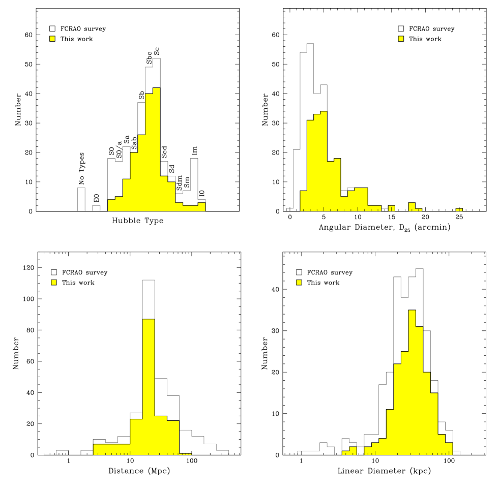
Figure 1: Distributions of morphological types (top left panel), optical angular diameters (top right panel), distances (bottom left panel) and linear diameters (bottom right panel): the solid portion of the histograms indicates the sub-sample used in this work (180 galaxies) whilst the empty portion indicates the distribution of the FCRAO CO survey (300 galaxies). Because of its outstanding angular size, the galaxy NGC598 (M33, $D_{25}=62\arcmin$) is not included in the histogram of angular diameters.

Distributions of morphological types, angular diameters, distances and linear diameters of the sample along with the corresponding distributions for the FCRAO CO survey are shown in Fig. 1.

The galaxies in our sample have morphological types ranging between S0 and I0. Most of them (89%) are spiral galaxies with morphological type between Sa-Sd.

The majority of the galaxies (about 90%) have an optical angular diameter (from RC2) $D_{25}\leq$10′, the median angular diameter being about 5′. This ensures that for all of them the NVSS properly recovered the flux density of the extended structures (see above). The remaining 20 galaxies have an optical angular diameter from 10′ to 25′. For these galaxies it is possible that the NVSS missed a significant fraction of flux from the extended structure. Because of its outstanding angular size, NGC598 (M33, $D_{25}=62\arcmin$) had been excluded from the analysis.

The distances of the galaxies in our sample (taken from Young et al. 1995) span from the Local Group up to about 80 Mpc. Over 87 galaxies are at the distance of the Virgo Cluster (20 Mpc).

The linear diameters range from $\sim 4$ to $\sim 100$ kpc. The median value is 31 kpc.

Our selection excluded most of the galaxies with an angular diameter less than 3′ , i.e. the intrinsically small galaxies (linear diameter smaller than 30 kpc) and the more distant ones.

The complete list of the galaxies in our study (including the galaxy name, Hubble type, inclination, angular diameter and distance) is available in electronic format at http://www.ira.bo.cnr.it/ $\sim$crapsi_s/RADIOCO/Article/tab_art.txt.

3 Data analysis

For each galaxy in our sample we extracted the radio surface brightness, $B_{1.4}$, from the NVSS images . We averaged the NVSS pixel values within circular regions of 45″ diameter, centered on the same pointing positions of the FCRAO survey. Following the same formalism adopted by RY99 for the H_α emission, the radio brightness is expressed in terms of the ratio between the radio luminosity at 1.4 GHz, $L_{1.4}$, and the de-projected surface, $\Sigma$, intercepted by the beam on the galaxy disk:

$$\frac{L_{1.4}\leavevmode\nobreak\ ({\rm W\leavevmode\nobreak\ Hz^{-1}})}{\Sigma\leavevmode\nobreak\ (\rm kpc^{2})}=3.2\times 10^{18}\leavevmode\nobreak\ B_{1.4}\left(\frac{\rm mJy}{\rm beam}\right)\leavevmode\nobreak\ \cos\leavevmode\nobreak\ i$$ (1)

where $i$ is the inclination angle of the galaxy with respect to the plane of the sky. The surface luminosity has the advantage to be distance independent as opposed to the global luminosity.

Since most of continuum radio luminosity of normal galaxies is produced by relativistic electrons accelerated by supernovae explosion and the supernova rate ($\nu_{\rm SN}$) is directly related to the SFR of massive stars, a relation is expected between the radio luminosity and the star formation rate. In the following we indicate with SFR the formation rate of stars with mass $M\geq 5M_{\odot}$. Condon (1992) calibrated empirically the $\nu_{\rm SN}$-SFR relation using the supernova rate and the radio luminosity of our Galaxy:

$$L_{\nu}\leavevmode\nobreak\ ({\rm W\leavevmode\nobreak\ Hz^{-1}})=5.3\times 10^{21}\nu_{\rm GHz}^{-\alpha}\cdot{\rm SFR}\leavevmode\nobreak\ ({\rm M_{\odot}yr^{-1}})$$ (2)

where a Miller-Scalo (1979) initial mass function (IMF) is assumed and $\alpha$ is the radio spectral index ($S_{\nu}\propto\nu^{-\alpha}$). Condon (1992) noted that this relation should apply to the majority of normal galaxies in order to be consistent with the tight FIR/radio correlation widespreadly observed.

Assuming for the radio spectral index a typical value of $\alpha=0.8$, from Eq. (1) and Eq. (2) the relation between the star formation rate per unit surface, $\Sigma_{\rm SFR}$, and the radio brightness at 1.4 GHz is found to be:

$$\Sigma_{\rm SFR}\left({\rm\frac{M_{\odot}}{yr\leavevmode\nobreak\ kpc^{2}}}\right)=8.0\times 10^{-4}\leavevmode\nobreak\ B_{1.4}\left(\frac{\rm mJy}{\rm beam}\right)\leavevmode\nobreak\ \cos\leavevmode\nobreak\ i$$ (3)

In order to derive the ${\rm H}_{2}$  surface density from the FCRAO CO survey integrated CO intensity $I_{\rm CO}$ , we used the formula (RY99):

$$\Sigma_{{\rm H_{2}}}({\rm M_{\odot}\leavevmode\nobreak\ pc^{-2}})=8.5\leavevmode\nobreak\ I_{\rm CO}({\rm K\leavevmode\nobreak\ km\leavevmode\nobreak\ s^{-1}})\leavevmode\nobreak\ \cos\leavevmode\nobreak\ i$$ (4)

In this formula it is assumed a constant linear conversion factor between the CO luminosity and ${\rm H}_{2}$  mass equal to $X_{\rm CO}=2.8\times 10^{20}\leavevmode\nobreak\ {\rm\leavevmode\nobreak\ H_{2}\leavevmode\nobreak\ cm^{-2}[K\leavevmode\nobreak\ km\leavevmode\nobreak\ s^{-1}]^{-1}}$ (Bloemen et al. 1986).

A realistic estimate of the uncertainties in both $\Sigma_{\rm SFR}$ and $\Sigma_{{\rm H_{2}}}$ surface densities should consider several systematic effects. The relation between the SFR and the radio luminosity is based on many not well proved assumptions, such as the IMF thresholds and slope and the extrapolation of the $\nu_{\rm SN}$-SFR Milky Way relation to other galaxies. Cram et al. (1999) pointed out that different modelling of these parameters introduce scaling uncertainties up to a factor of 2. The dominant errors in the gas density are the variation on the CO/${\rm H}_{2}$ conversion factor. These variations can be as high as $\pm$40% for luminous spiral galaxies as those studied in this work (Devereux & Young 1991). Despite these uncertainties, the data provide very strong constrains on the form of the SFE because of the wide ranges of SFR and gas densities explored.

Consistently with the definition given by RY99, the radio SFE is calculated by the ratio of $\Sigma_{\rm SFR}$ to $\Sigma_{\rm H_{2}}$ . In terms of our observables ($B_{1.4}$ and $I_{\rm CO}$ ) the SFE is expressed by

$${\rm SFE\leavevmode\nobreak\ (yr^{-1})}\equiv\frac{\Sigma_{\rm SFR}}{\Sigma_{\rm H_{2}}}=9.4\times 10^{-11}\leavevmode\nobreak\ \frac{B_{1.4}}{I_{\rm CO}}$$ (5)

where $B_{1.4}$ and $I_{\rm CO}$ are measured in mJy/beam and K km s^-1, respectively.

The SFE defined by Eq. (5) gives the fraction of molecular gas converted to massive stars per year. Since the typical lifetime of the synchrotron radiating electrons is shorter than $10^{8}$ yr (Condon 1992), the SFR inferred from the radio luminosity traces a stellar population not older than this timescale (hereafter $\tau_{8}$). The percentage of molecular gas consumed over all this period is

$${\rm SFE_{\tau_{8}}(\%)}=0.94\leavevmode\nobreak\ \frac{B_{1.4}}{I_{\rm CO}}$$ (6)

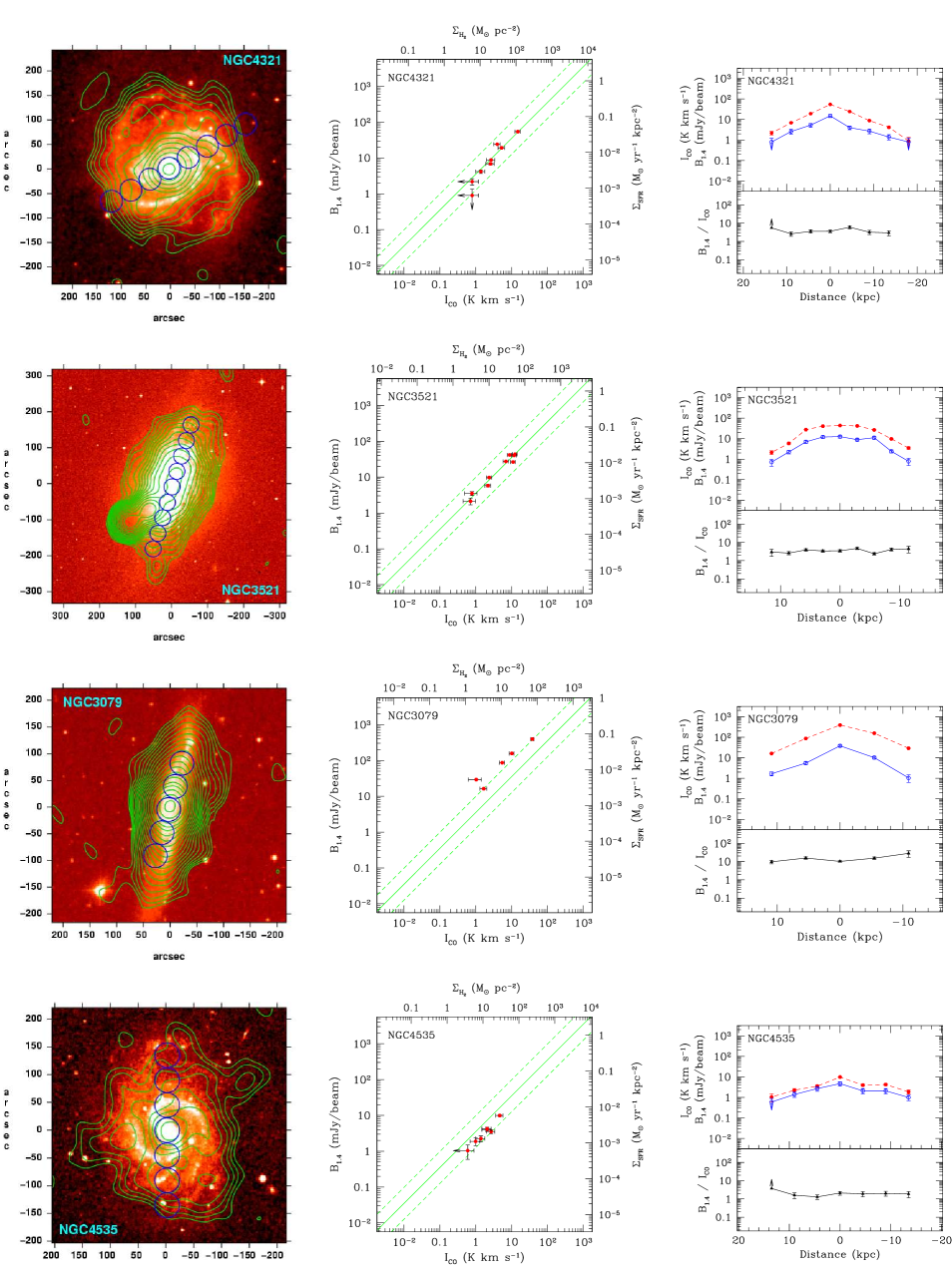
Figure 2: Examples of selected galaxies, see text. Solid and short-dashed lines in middle panels refer to the mean and standard deviation of the ${\rm SFE_{\tau_{8}}}$ of the entire sample. Solid and dashed lines in right panels refer to $I_{\rm CO}$ an $B_{1.4}$ profiles, respectively.

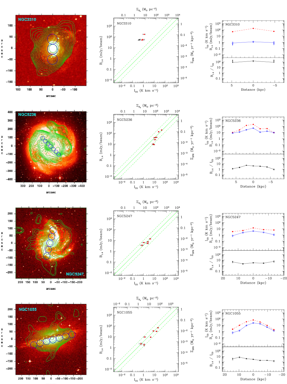
Figure 3: Examples of selected galaxies, see text. Solid and short-dashed lines in middle panels refer to the mean and standard deviation of the ${\rm SFE_{\tau_{8}}}$ of the entire sample. Solid and dashed lines in right panels refer to $I_{\rm CO}$ an $B_{1.4}$ profiles, respectively.

4 Results

The data analysis presented in Sec. 3 allows one to compare the SFR and the molecular gas content to determine the star formation efficiency along the galaxy disks.

Overlays of optical (grayscale) and radio continuum (contours) images for eight selected galaxies are shown in the left columns of Figs. 2 and 3, where the circles indicate the positions and the beam size of the CO observation. In the middle columns we plot $B_{1.4}$ versus $I_{\rm CO}$ reporting also the corresponding values of $\Sigma_{\rm SFR}$ and $\Sigma_{{\rm H_{2}}}$ in the upper and right axis, respectively. The panels in the right columns show the radio brightness ($B_{1.4}$), the CO integrated intensity ($I_{\rm CO}$ ) and their ratio as a function of distance from the galaxy center. The convention is that radius is positive for positive right ascension (or declination) pointing shifts. The optical images are taken from the red Palomar Digitized Sky Survey. The NVSS radio contours start at 0.9 mJy beam^-1 ($2\sigma$) and are spaced by a factor of $\sqrt{2}$. In the plots, error bars and arrows indicate respectively measurement uncertainties and upper limits ($2\sigma$). In the middle column panels, the reference lines represent the mean (solid) and standard deviation (short-dashed) of the SFE computed using all the detections in the whole sample (see Sect. 4.2). In right column panels, the dashed and continuous lines show the $B_{1.4}$ and $I_{\rm CO}$ trends, respectively.

Figure 4: Histogram of star formation efficiency at 628 pointing positions for the entire sample. Only points with a signal-to-noise ratio greater than 2$\sigma$ have been considered. Mean and dispersion refer to the logarithmic values of ${\rm SFE_{\tau_{8}}}$, see text. Values greater than 100% indicate present SFRs that cannot be supported for more than $10^{8}$ yr.

4.1 The SFE within galaxy disks

Most of the galaxies in our sample are at distances between 10 and 40 Mpc, the corresponding linear resolution of the 45″ beam is between 2.2 and 8.7 kpc, i.e. so large to sample the contribution from many molecular clouds complexes. In the following, one should keep in mind that the star-forming regions we are observing are comparable with the width of the spiral arms only for the nearest objects.

The galaxies shown in Figs. 2 and 3 are representative of the diversity of behaviour seen in the distributions of $B_{1.4}$ and $I_{\rm CO}$ within galaxy disks.

The most striking feature is the linear correlation between these two quantities observed for many edge-on and face-on galaxies (see Fig. 2). In these cases, $B_{1.4}$ and $I_{\rm CO}$ present the same scaling from the galaxy center outward, resulting in a constancy of the SFE along the disk. However, there are clear examples of disks characterized by systematic SFE trends (see Fig. 3). A $B_{1.4}$ gradient steeper (flatter) with respect to $I_{\rm CO}$ one implies a SFE decreasing (increasing) with radius (e.g. NGC5236 and NGC5247). Calculating the SFR from non-thermal radio continuum allows us to include in the analysis high inclined galaxies, such as NGC1055 and NGC3079, which generally suffer from extinction in the optical band (see Sect. 5.1). By fitting a power law of the form $B_{1.4}\propto{I_{\rm CO}}^{N}$, we found that the fraction of linear ($0.5<N<2$) correlations is 67%, while the fractions of super-linear ($N>2$) and sub-linear ($N<0.5$) correlations are 23% and 10%, respectively. We examine the composite correlation including all the pointings in the sample in Sect. 4.3.

Figure 5: Histograms of star formation efficiency sorted by galaxy type. Only points with a signal-to-noise ratio greater than 2$\sigma$ have been considered. Mean and dispersion refer to the logarithmic values of ${\rm SFE_{\tau_{8}}}$, see text.

4.2 The SFE variation among galaxies

Having established a correlation between the radio continuum surface brightness and the CO line intensity within galaxies, we investigated the variation of the SFE among galaxies. Fig. 4 shows the distribution of the ${\rm SFE_{\tau_{8}}}$ for the galaxy sample. ${\rm SFE_{\tau_{8}}}$varies from about 0.1 up to more than 100%. Values greater than 100% indicate present SFRs that cannot be supported for more than $10^{8}$ yr. Since the distribution of logarithmic values is more Gaussian we calculated the mean and the dispersion of $\log$(${\rm SFE_{\tau_{8}}}$). The mean of $\log$(${\rm SFE_{\tau_{8}}}$) is approximately 3.5% of the gas consumed per 10⁸ yr and the rms of the distribution is slightly less than a factor of 3. ${\rm SFE_{\tau_{8}}}$ mean and dispersion of the sample are traced in middle plots of Figs. 2 and 3 as solid and dashed reference lines, respectively.

We examined also the variation of ${\rm SFE_{\tau_{8}}}$ among galaxies compared to the morphological type (see Fig. 5).The mean star formation efficiency varies weakly (about 25%) with the morphological type going from S0 to Scd galaxies.

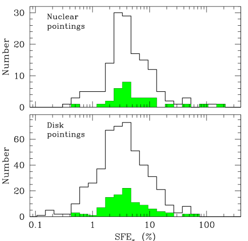
Figure 6: Histograms of star formation efficiency for nuclear (top panel) and disk (bottom panel) pointings. The solid line and solid portion of the histograms indicate normal and Seyfert galaxies, respectively. Three galaxies have nuclear ${\rm SFE_{\tau_{8}}}$ greater than 100%; namely NGC2655, NGC3310 and NGC4151. NGC2655 and NGC4151 are classified as Sy2 and Sy1.5 and have nuclear ${\rm SFE_{\tau_{8}}}$ of 100% and 170%, respectively. The galaxy NGC3310 is a peculiar starburst galaxy characterized by an exceptional nuclear ${\rm SFE_{\tau_{8}}}$ of about 135%

Larger SFE close to the galaxy centers might be attributed to the presence of an active nucleus (AGN). Fig. 6 shows the distribution of disk and nuclear ${\rm SFE_{\tau_{8}}}$ in Seyfert and normal galaxies. Seyferts have a slightly higher ${\rm SFE_{\tau_{8}}}$ than normal galaxies. The mean of the log ${\rm SFE_{\tau_{8}}}$, for Seyfert and normal galaxies, is: 4.1% and 3.3% in the disks and 5.5% and 4.3% in the nuclei, respectively. Most Seyferts have a nuclear ${\rm SFE_{\tau_{8}}}$ comparable with normal galaxies. Only in few cases the nuclear emission is dominated by the radio source related with the AGN, e.g. NGC1068 (Wilson & Ulvestad 1987), NGC4151 (Pedlar et al. 1993), NGC2655 (Keel & Hummel 1988) and NGC4388 (Irwin et al. 2000). We conclude that the AGN-related emission affects only marginally the estimate of the ${\rm SFE_{\tau_{8}}}$ in the nuclear pointings for most Seyfert in our sample.

We further investigate the behaviour of the SFE with respect to the galaxy inclination and size, and beam linear resolution. Fig. 7 shows the maximum variation of the ${\rm SFE_{\tau_{8}}}$, defined as SFE_max/SFE_min, inside each galaxy. Most galaxies present SFE variation up to a factor 6, the median variation being a factor of 2.5.

Figure 7: Star formation efficiency variations within each galaxy as a function of inclination (top panel) and linear resolution of the 45″ beam (bottom panel). Seyfert galaxies are distinguished with open dots. The majority of galaxies have internal SFE variation less than a factor of 3. The starburst galaxies NGC3034 (M82) and NGC520 and the HII galaxy NGC6503, have exceptional internal SFE variations (larger than a factor of 30).

Fig. 7 shows that the internal SFE variations are not strong function of the galaxy inclination or linear resolution of the observing beam. Considerable SFE variations occur also for size of the beam greater than 5 kpc, i.e. smoothing over large regions of the galaxy disks. This fact was already noted by RY99. Ten galaxies show an internal SFE variation greater than a factor of 10. These are: the circumnuclear starbursts IC342, NGC253, NGC520, NGC660, NGC2146 and NGC3034 (see Kennicutt 1998); the Seyfert galaxies NGC2841 and NGC3368; the peculiar galaxy NGC3628; the HII galaxy NGC6503. M82, NGC520 and NGC6503, show exceptional internal SFE variations larger than a factor of 30. In particular, the nearby starburst M82 show a variation of about 2.6 order of magnitude.

Finally, we investigated the behaviour of the star formation efficiency as a function of the distance from the galaxy centers. Fig. 8 shows the SFE as a function of radius for all galaxies. The SFE is found to be approximately constant at all radii.

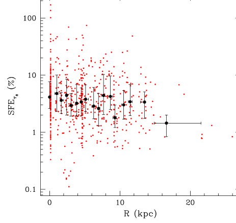
Figure 8: Star formation efficiency as a function of radius for all galaxies. Limits are not shown. All the detections are represented as small points. Bold points and error bars represent the median value and the 50% of objects in each bin, respectively.

4.3 The composite radio Schmidt law

Our data offer the possibility to determine the spatially resolved Schmidt law using the radio continuum as SFR indicator for a sample of galaxies six times larger than the one of Adler et al. (1991). Fig. 9 shows the relationship between the SFR and the ${\rm H}_{2}$ surface densities for all the pointings of the sample. Dashed and dotted reference lines indicate the mean and standard deviation of the ${\rm SFE_{\tau_{8}}}$ for all the detection in the sample (see Sect. 4.1). The galaxies NGC4302, NGC4526, NGC4710 and NGC4866 have been omitted since they have inclination $i=90\degr$. A clear correlation is evident over more than three orders of magnitude, albeit a consistent scatter of 0.5 dex is present. We stress once more that, since this is a correlation between two brightness, we can rule out any subtle effect introduced by the distance. This result confirms the correlation found by Adler et al. (1991) on global scales. The best weighted fit of the radio Schmidt law, $\Sigma_{{\rm SFR}}=a\times{\Sigma_{{\rm H_{2}}}}^{N}$, is: $a=2.6(\pm 1.2)\times 10^{-4}$ and $N=1.3\pm 0.1$. The value for the exponent of the radio Schmidt law is fully consistent with both the global (e.g. Kennicutt 1998) and local (RY99) slopes found using the H_α line emission as SFR indicator. This exponent for the Schmidt law indicates a SFE which weakly increases with the SFR.

Figure 9: Spatially resolved radio Schmidt law for all the detections in the sample. Arrows indicate upper limits at 2$\sigma$. The solid line is the best fit of the composite radio Schmidt law: $\Sigma_{{\rm SFR}}\propto{\Sigma_{{\rm H_{2}}}}^{1.3}$. Dashed and dotted lines refer to the mean and standard deviation of the ${\rm SFE_{\tau_{8}}}$ for all detections in the sample: 3.5% and a factor of 2.8 respectively. The galaxies NGC4302, NGC4526, NGC4710 and NGC4866 have been omitted since they have inclination $i=90\degr$.

5 Discussion and conclusions

The most striking result of our study is the overall consistency of the SFE obtained from the 20 cm radio continuum as SFR indicator instead of the H_α  emission (RY99). Basically we found all the essential features observed by RY99: the constancy of the SFE both within and among galaxies; the weak dependence of the SFE on morphological type and linear size of the observing beam; the extent and slope of the composite Schmidt law. Nevertheless, some important differences arise. In this section we present in details the differences between the two works, discussing their nature and implications.

Figure 10: Comparison of SFRs surface densities deduced from 1.4 GHz luminosity (horizontal axis) and H_α emission (vertical axis) for 102 galaxies of our sample in common with RY99. The various panels show different values of galaxy inclinations $i$, as indicated. There are 453 detections, 65 of which are upper limits (at 2$\sigma$). The reference dashed lines indicate 1:1 relations. The subsample of face-on galaxies ($i\leq 40\degr$) shows the best correlation, with a dispersion of a factor of 2.3. SFRs surface densities deduced by the H_α for highly inclined galaxies ($i\geq 70\degr$) are systematically underestimated for $\Sigma_{\rm SFR}{\rm 1.4\leavevmode\nobreak\ GHz}\geq 3\times 10^{-3}\leavevmode\nobreak\ {\rm M_{\odot}\leavevmode\nobreak\ yr^{-1}kpc^{-2}}$.

5.1 Star formation rate surface densities

Cram et al. (1998) checked the consistency between the SFR deduced from the radio luminosity with the rates predicted by other indicators, in particular by the H_α luminosity. They concluded that the rates deduced from the radio continuum and the H_α luminosities, although in broad agreement, are affected by two systematic deviations: respectively at low ($\leq 0.1\leavevmode\nobreak\ {\rm M_{\odot}yr^{-1}}$) and high ($\geq 20\leavevmode\nobreak\ {\rm M_{\odot}yr^{-1}}$) star formation rates, the H_α luminosity overestimate and underestimate the SFR deduced by the radio luminosity. The deviation at low rates can be attributed in part to problems related to the zero-point H_α luminosity calibration. They suggest that the deviation at high SFR could be attributed to a larger amount of extinction by dust in those objects undergoing strong star formation or to particular IMFs that favour low mass supernovae progenitors rather than high mass stars responsible for the H_α .

By comparing our data set with that of RY99 we have the possibility to extend the consistency check between the surface star formation rate densities deduced from the radio continuum and H_α emission over the same regions of galaxy disks.

Figure 11: Ratio of SFRs surface densities deduced from H_α and 1.4 GHz luminosity for highly inclined (NGC1055 and NGC3079) and starburst galaxies (NGC2146, NGC3034). These examples dramatically illustrate that the SFRs surface density inferred from the H_α emission towards the nuclei of these objects are underestimated by more than one order of magnitude.

Using Eq. (2) of Cram et al. (1998), we calculated the SFR surface density from the H_α brightness reported by RY99 through the formula:

$$\Sigma_{\rm SFR}\left({\rm\frac{M_{\odot}}{yr\leavevmode\nobreak\ kpc^{2}}}\right)=2.6\times 10^{-2}\leavevmode\nobreak\ \mu({\rm H_{\alpha}})$$ (7)

where the (de-projected) H_α surface brightness, $\mu({\rm H_{\alpha}})$, is measured in ${\rm L_{\odot}\leavevmode\nobreak\ pc^{-2}}$. Eq. (2) of Cram et al. (1998) accounts for a correction of 1.1 magnitude in the luminosity to compensate for the mean extinction in H_α (Kennicutt 1983a). Fig. 10 shows the direct comparison between the radio and H_α SFRs inferred respectively from Eq. (3) and Eq. (7) for 453 position within 102 galaxies of the sample. All galaxies are shown in the top panel of Fig. 10. In general there is a broad agreement between the two SFR indicators. Considering the distribution of the logarithm values of the ratio $R=\Sigma_{\rm SFR(H_{\alpha})}/\Sigma_{\rm SFR(1.4GHz)}$, we have that $R$ have a mean of 0.83 with a standard deviation of 2.8, i.e. the H_α is underestimating the surface SFR as compared to continuum radio emission. Sorting the sample by galaxy inclination indicates that this effect is strongly correlated with galaxy orientation. For the face-on subsample ($i<40\degr$) $R$ has a mean of 1.1 and a dispersion of a factor 2.3. At intermediate inclinations ($40\degr\leq i<70\degr$) mean and dispersion of $R$ are 0.8 and a factor of 3, respectively. Finally, for highly inclined galaxies ($i\geq 70\degr$) mean and dispersion of $R$ are 0.7 and a factor of 2.9, respectively. In particular, SFR surface densities deduced by the H_α for highly inclined galaxies are systematically underestimated for $\Sigma_{\rm SFR(1.4\leavevmode\nobreak\ GHz)}$ greater than $\sim 3\times 10^{-3}\leavevmode\nobreak\ {\rm M_{\odot}\leavevmode\nobreak\ yr^{-1}kpc^{-2}}$. Fig. 11 shows two edge-on spirals, NGC3079 and NGC1055 (see Figs. 2 and 3) and two well known starburst galaxies, NGC2146 and M82, in which SFRs deduced by the H_α emission are underestimated by more than a factor of about 10. As a consequence, the SFE variations deduced for these objects by RY99, on the basis of H_α observations, can be attributed to extinction, as suspected by these authors.

These results have two important implications: i) the close correlation observed between $\Sigma_{\rm SFR(1.4\leavevmode\nobreak\ GHz)}$ and $\Sigma_{\rm SFR(H_{\alpha})}$ for face-on galaxies reinforces the use of the radio luminosity as SFR indicator not only on global but also on local scales; ii) extinction could significantly affect estimates based on H_α emission for high SFRs in edge-on galaxies.

Although the star formation rates deduced from the H_α emission are systematically underestimated compared to those deduced from the radio continuum, the mean SFE reported by RY99 for their entire sample (121 galaxies) is 4.3%, i.e. higher than the mean SFE deduced from the radio continuum for our entire sample of 180 galaxies. However, considering the 103 galaxies we have in common with RY99, the mean SFE deduced from the H_α emission is about 3.1% in good agreement with our value.

Figure 12: Ratio of SFRs surface densities deduced from 1.4 GHz luminosity and H_α emission as functions of the linear scale of the beam (top panel) and distance from galaxy center (bottom panel). Highly inclined galaxies ($i>70\degr$) are represented with open dots.

5.2 Non-thermal radio continuum scale-length

Discrete supernova remnants (SNR) themselves account only for $<10\%$ of the radio luminosity of normal galaxies (Ilovaisky & Lequeux 1972). Most of cosmic rays escape from their parent SNRs and diffuse along the galaxy disk during their characteristic lifetimes which are much larger than typical ages of SNRs ($\sim 10^{5}$ yr). Therefore one expects the non-thermal radio continuum emission to be smoothed over a larger region around the parent stellar population with respect to the H_α emission. On scale smaller than the cosmic rays characteristic diffusion scale, $D_{\rm CR}$, the non-thermal radio continuum cannot provide a reliable estimate of the local SFR. On the other hand, averaging over regions larger than the typical spiral arm width leads to a dilution of the H_α emission. Fig. 12 (top panel) shows the ratio between the SFR surface densities deduced from H_α and from radio luminosity versus linear size of the observing beam. One notes that, apart for edge-on galaxies (where the H_α is affected by extinction), the ratio $\Sigma_{\rm SFR(1.4\leavevmode\nobreak\ GHz)}$ to $\Sigma_{\rm SFR(H_{\alpha})}$ tends to increase with the beam size. In particular, the ratio is smaller or greater than one for beam sizes respectively below and above $\sim 5$ kpc. This is consistent with a scenario in which the characteristic linear scale of both cosmic rays diffusion scale and arm size is about 3 kpc. Higher resolution radio images are required to determine the lowest linear scale at which the radio continuum correlates with the H_α emission and thus providing an estimate of $D_{\rm CR}$.

We found also that the ratio $\Sigma_{\rm SFR(1.4\leavevmode\nobreak\ GHz)}$ to $\Sigma_{\rm SFR(H_{\alpha})}$ on average does not depend on the distance from the galaxy centers (Fig. 12, bottom panel).

5.3 The nature of Schmidt law scatter

The dispersion (standard deviation) of the composite radio Schmidt law shown in Fig. 9 is a factor of 2.8, which is smaller than the corresponding dispersion of a factor 4 of the H_α Schmidt law (RY99). This is probably because the radio continuum does not suffer the effects of dust extinction. The noisiness of the correlation could reflect real variations of the mean Schmidt law, indicating that it should be regarded at best as a first order approximation of the star formation process, or it could be due to the many assumptions involved in the calculation of gas and SFR densities.

Variations of the $X_{\rm CO}$ factor from galaxy to galaxy can be advocated to explain a part of the correlation scatter. These could introduce uncertainties up to a factor of 2 in the gas density scale (Kennicutt 1998). Another possibility is that the extrapolation of the proportionality between CO luminosity and virial mass of giant molecular clouds observed in our own Galaxy and in nearby galaxies, which is the basis of molecular mass determinations in this and similar works, does not hold for all spiral galaxies.

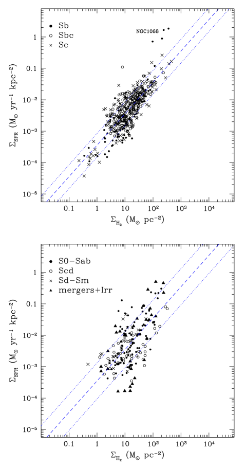
Figure 13: Radio Schmidt law for Sa, Sbc and Sc (top panel) and S0-Sab, Scd, Sd-Sm and merging-irregular (bottom panel); limits are not shown. Dashed and dotted reference lines indicate the mean and the dispersion of the two sub-samples, respectively. The scatter of the Schmidt law is considerably reduced excluding extreme morphological types. The scatter of the correlations shown in top and bottom panels is a factor of 2.4 and 3.8, respectively. In top panel, the deviation from the correlation of the four points belonging to NGC1068 is due to the AGN-related radio emission of this Seyfert galaxy (see Sect. 4.2).

However, by comparing SFR surface densities deduced from H_α and from radio continuum luminosity we showed that, even in the face-on subsample, the $\Sigma_{\rm SFR(H_{\alpha})}-\Sigma_{\rm SFR(1.4\leavevmode\nobreak\ GHz)}$ relation itself is affected by a scatter of at least a factor of 2. Hence, the uncertainties of the SFR indicators alone can account for a consistent fraction of the Schmidt law scatter.

Fig. 13 shows the Schmidt law separately for Sb, Sbc and Sc and S0-Sab, Scd and Sd-Sm galaxies (only detections with signal-to-noise ratio greater than 2$\sigma$ are considered). The two subsamples have the same mean SFE of 3.5% but very different dispersions of a factor of 2.4 for the former and 3.8 for the latter, i.e. the scatter of the Schmidt law is considerably reduced excluding extreme morphological types. RY99 also found that the H_α Schmidt law is considerably tightened with the exclusion of the irregular galaxies and mergers. These SFE variations around the mean Schmidt law can be attributed to the particular physical conditions and/or environments experienced by these objects (see e.g. starburst galaxies), but they could also be induced by observational effects further amplified by poor statistic. In fact, Scd galaxies which are characterized by the lower mean SFE in our sample (see also Fig. 5) behave consistently with other morphological types excluding IC342 for which the NVSS misses flux density from the extended structure, see Sec. 2.

5.4 Molecular gas consumption timescale

The star formation efficiency can be expressed in terms of gas consumption (or cycling) timescale. The molecular gas consumption timescale, $\tau_{\rm H_{2}}$, indicates the time needed to convert all the molecular gas in stars given a constant SFE. Expressed in Gyr, $\tau_{\rm H_{2}}$ is given by

$$\tau_{\rm H_{2}}({\rm Gyr})=\frac{10}{\rm SFE_{\tau 8}(\%)}$$ (8)

The mean star formation efficiency found in this work for spiral galaxies yields a molecular gas consumption timescale of about $\tau_{\rm H_{2}}\simeq 2.8$ Gyr. Given the dispersion of the SFE in the sample, most galaxies have gas cycling timescale between about 1 and 9 Gyr. At the lower end of the distribution we found galaxies with a ${\rm SFE_{\tau_{8}}}$$\sim 1\%$, such as NGC4535 (see Fig. 2). The corresponding molecular gas consumption timescale is almost comparable with the Hubble time. The shortest gas cycling timescale corresponds to galaxies with exceptional SFE like NGC3310 (see Fig. 3). Star formation rates in these galaxies are so high, compared to their gas supplies, that the gas cycling timescale is $\tau_{\rm H_{2}}\leq 0.1$ Gyr.

It is interesting to investigate the behaviour of the so-called starburst galaxies with respect to the gas cycling timescale. In literature, galaxies have been classified as starbursts according to different criteria. Heckman et al. (1998) define a galaxy as starburst when it is hosting a star-forming event that dominates its bolometric luminosity, i.e. on the basis of the magnitude of the SFR. Alternatively, Shu (1987) and Young (1987) proposed a classification based on the efficiency of the star formation. In this latter definition a galaxy with a high SFR is not defined as starburst if the mass of gas available is enough to sustain the star formation rate and vice versa. Following RY99 we selected the galaxies hosting a region in which the SFE is enhanced by a factor of three compared to the mean of the sample; for these starburst regions $\tau_{\rm H_{2}}\leq 1$ Gyr. Fig. 14 shows the usual $\Sigma_{{\rm SFR}}-\Sigma_{{\rm H_{2}}}$ plane for all the detection in the sample along with three reference lines indicating the gas cycling timescales $\tau_{\rm H_{2}}=0.1$, 1 and 10 Gyr.

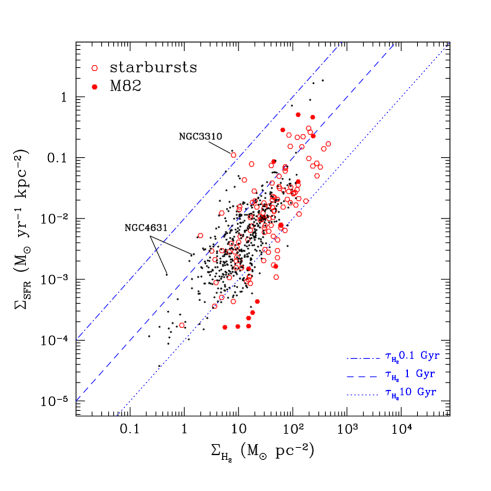
Figure 14: $\Sigma_{{\rm SFR}}-\Sigma_{{\rm H_{2}}}$ plane for all the detection in the sample (limits are not shown) along with three reference lines corresponding to different molecular gas consumption timescales, as indicated. Pointings of known starburst galaxies are represented by open dots.

Most galaxies known in literature as “starbursts” have consumption timescales comparable with those of normal spiral galaxies. In some cases, e.g. M82, starburst galaxies host both regions characterized by SFE lower and higher than the mean of the sample. On the other hand, galaxies with normal or even low SFR surface densities, such as the highly inclined galaxy NGC4631, should be regarded as starburst according to our selection criterion based on the SFE. Finally, there are some galaxies for which the SFE is so high that the gas cycling timescale is $\tau_{\rm H_{2}}\leq 0.1$ Gyr, e.g. the starburst NGC3310. NGC3310 is one of the best examples of a local UV-bright starburst (see Conselice et al. 2000 and reference therein). The exceptional high SFE of this galaxy indicates that its interstellar medium is truly affected by an extraordinary star formation event.

5.5 Conclusions

The results of this work are the following:

1. There is a tight correlation between the 20 cm non-thermal radio continuum and the CO line intensity in a representative sample of 180 spiral galaxies. The correlation holds within and among the galaxies.

2. The mean star formation efficiency, i.e. the ratio of the radio SFR to the molecular gas densities, for our sample is $0.035\times 10^{-8}$ yr^-1 with a dispersion of a factor of 3. This corresponds to convert 3.5% of the available gas into stars on a time of $10^{8}$ yr.

3. The comparison of SFRs surface densities deduced from 1.4 GHz luminosity and from the H_α emission for 102 galaxies, reveals that $\Sigma_{\rm SFR(1.4\leavevmode\nobreak\ GHz)}$ and $\Sigma_{\rm SFR(H_{\alpha})}$ are closely correlated for face-on galaxies ($i\leq 40\degr$), reinforcing the use of the radio radio luminosity as SFR indicator not only on global but also on local scales. SFRs surface densities deduced by the H_α luminosity for highly inclined galaxies ($i\geq 70\degr$) are systematically underestimated for $\Sigma_{\rm SFR(1.4\leavevmode\nobreak\ GHz)}\geq 3\times 10^{-3}\leavevmode\nobreak\ {\rm M_{\odot}\leavevmode\nobreak\ yr^{-1}kpc^{-2}}$.

4. The star formation efficiency varies weakly (less than 25%) with the Hubble morphological type.

5. The variation of the SFE within individual galaxy disks is less than a factor of 3. The largest variations are found in starburst galaxies.

6. The SFE is found to be approximately constant as a function of distance from the galaxy centers.

7. The composite radio Schmidt law, star formation versus molecular gas content, extends for more than 3 order of magnitude with an exponent of 1.3.

8. Most galaxies known in literature as “starbursts” have consumption timescales comparable with those of normal spiral galaxies. In some cases, e.g. M82, starburst galaxies host both regions characterized by a SFE lower and higher than the mean of the sample. Furthermore, there are some galaxies for which the SFE is so high that the gas cycling timescale is $\tau_{\rm H_{2}}\leq 0.1$ Gyr, e.g. NGC3310.

- (1) Adler, D.S., Allen, R.J., Lo, K.Y., 1991, ApJ 238, 475
- Bloemen et al. (1986) Bloemen, J.B.G.L., Strong, A.W., Mayer-Hasselwander, H.A., et al., 1986, A&A, 154, 25
- (3) Condon, J.J., 1992, ARA&A, 30, 575
- (4) Condon, J.J., Cotton, W.D., Greisen, E.W., et al., 1998, AJ, 115, 1693
- (5) Conselice, C.J., Gallagher, J.S., Calzetti, D., et al., 2000, AJ, 119, 79
- (6) Cram, L., Hopkins, A., Mobasher, B., et al., 1998, ApJ, 507, 155
- (7) de Vaucouleurs, G., de Vaucouleurs, A., Corwin, J.R., 1976, Second Refrence Catalogue of Bright Galaxies (Austin: Univ. of Texas Press) (RC2)
- (8) Devereux, N.A., & Young, J.S., 1991, ApJ, 371, 515
- (9) Heckman, T., Carmelle, R., Leitherer, C., et al., 1998, ApJ, 503, 646
- (10) Ilovaisky, S.A., & Lequeux, J., 1972, A&A, 20, 347
- (11) Irwin, J.A., Saikia, D.J., English, J., 2000, AJ, 119, 1592
- (12) Keel, W.C., & Hummel, E., 1988, A&A, 194, 90
- (13) Kennicutt, R.C., 1983a, ApJ, 272, 54
- (14) Kennicutt, R.C., 1998, ApJ, 498, 541
- (15) Lequeux, J., 1971, A&A, 15, 42
- (16) Miller, G.E., & Scalo, J.M., 1979, ApJS, 41, 513
- (17) Pedlar, A., Kukula, M.J., Longley, D.P.T., et al., 1993, MNRAS, 263, 471
- (18) Rownd, B.K., & Young, J.S., 1999, AJ, 118, 670
- (19) Schmidt, M., 1959, ApJ, 129, 243
- (20) Shu, F.H., 1987, in Star Formation in Galaxies, ed. C.J. Lonsdale Persson (NASA CP - 2466)(Washington: NASA), 263
- (21) Tacconi, L., & Young, J.S., 1986, ApJ, 308, 600
- (22) Wilson, A.S., & Ulvestad, J.S., 1987, ApJ, 319, 105
- (23) Young, J.S., 1987, in Star Formation in Galaxies, ed. C.J. Lonsdale Persson (NASA CP - 2466)(Washington: NASA), 197
- (24) Young, J.S., & Scoville, N.Z., 1991, ARA&A, 29, 581
- (25) Young, J.S., Xie, S., Tacconi, L., et al., 1995, ApJS, 98, 219