Extended Power-Law Decays in BATSE Gamma-Ray Bursts:
Signatures of External Shocks?

Abstract

The connection between Gamma-Ray Bursts (GRBs) and their afterglows is currently not well understood. Afterglow models of synchrotron emission generated by external shocks in the GRB fireball model predict emission detectable in the gamma-ray regime ($\mathrel{\hbox{\raise 2.15277pt\hbox{$>$}\hbox to0.0pt{\hss\lower 2.15277pt\hbox{$\sim$}}}}25$ keV). In this paper, we present a temporal and spectral analysis of a subset of BATSE GRBs with smooth extended emission tails to search for signatures of the “early high-energy afterglow”, i.e., afterglow emission that initially begins in the gamma-ray phase and subsequently evolves into X-Ray, uv, optical, and radio emission as the blast wave is decelerated by the ambient medium. From a sample of 40 GRBs we find that the temporal decays are best described with a power-law $\sim t^{\beta}$, rather than an exponential, with a mean index $\langle\beta\rangle\approx-2$. Spectral analysis shows that $\sim 20\%$ of these events are consistent with fast-cooling synchrotron emission for an adiabatic blast wave; three of which are consistent with the blast wave evolution of a jet, with $F_{\nu}\sim t^{-p}$. This behavior suggests that, in some cases, the emission may originate from a narrow jet, possibly consisting of “nuggets” whose angular size are less than $1/\Gamma$, where $\Gamma$ is the bulk Lorentz factor.

1. Introduction

Afterglow emissions from Gamma-Ray Bursts (GRBs) in the X-ray, optical, and radio wavebands are in good agreement with afterglow models of relativistic fireballs (Wijers, Rees, and Mészáros (1997), Galama et al. (1998), Waxman (1997), Vietri (1997)). The observed afterglow spectrum is well-described as synchrotron emission that arises from the interaction of the relativistic blast wave with bulk Lorentz factor $\Gamma_{0}\sim 10^{2}-10^{3}$ with the ambient medium (Mészáros and Rees (1997), Galama et al. (1998)). The often highly variable gamma-ray phase of the burst may reflect the physical behavior of the fireball progenitor through collisions internal to the flow, i.e., internal shocks (Sari and Piran (1997), Kobayashi et al. (1997)). On the other hand, Dermer and Mitman (1999) have suggested a blast wave with an inhomogenous external medium. Heinz and Begelman (1999) have suggested an inhomogeneous bullet-like jet outflow that encounters the interstellar medium.

The precise relationship between the observed GRB and the afterglow emission is not well understood. GRBs recorded by the BeppoSAX satellite suggest that the X-ray afterglow emission may be delayed in time from the main GRB (e.g., GRB970228, Costa et al. (2000)) or may begin during the GRB emission (e.g., GRB980519, In’T Zand et al. (1999)). In the latter case, it is not clear if the X-ray afterglow is a separate underlying emission component or a continuation of the GRB itself. The internal-external shock model presents a scenario in which emission from internal and external shocks may overlap in time. If the internal shocks reflect the activity of the progenitor, then the onset of the afterglow may be separated from the prompt gamma-ray emission. Since the nature of the progenitor is not known, the effect of the ambient medium on the emission from the progenitor is highly problematic. The model therefore does not prohibit internal and external shock emissions from overlap, while in other cases the afterglow emission may be delayed with respect to the GRB (e.g., Sari and Piran (1999), Mészáros and Rees (1999), Vietri (2000)).

The detection of optical emission simultaneous with the gamma-ray emission of GRB990123 (Akerlof et al. (1999)) provided the first evidence for two distinct emission components in a GRB; here, the prompt optical emission is believed to originate from synchrotron emission in the production of the reverse shock generated when the ejecta encounters the external medium (Galama et al. (1999), Sari and Piran (1999), Mészáros and Rees (1999)). The gamma-ray spectrum of GRB990123 can not be extrapolated from the spectral flux from the simultaneous optical emission, indicating that the optical and gamma-ray emission originate from two separate mechanisms (Briggs et al. (1999), Galama et al. (1999)). Evidence for overlapping shock emission was also found in GRB980923 (Giblin et al. 1999a ), where a long power-law decay tail ($\sim t^{-1.8}$) was observed in soft gamma-rays (25-300 keV). Two separate emission components are favored in this burst because the spectral characteristics of the tail were markedly different from those of the variable main GRB emission. The spectrum in the tail is consistent with that of a slow-cooling synchrotron spectrum, similar to the behavior of low-energy afterglows (e.g., Bloom et al. (1998), Vreeswijk et al. (1999)).

The gamma-rays produced by internal shocks and the soft gamma-rays of the “afterglow” may therefore overlap, the latter having a signature of power-law decay in the synchrotron afterglow model. If this is the case, at least some GRBs in the BATSE database should show signatures of the early external shock emission. These events would contain a soft gamma-ray (or hard X-ray) tail component that decays as a power-law in their time histories, possibly superposed upon the variable gamma-ray emission. It has been shown that the peak frequency of the initial synchrotron emission, which depends on the parameters of the system (see $\S 2$), can peak in hard X-rays or gamma-rays (Mészáros and Rees (1992)). Further, it may be possible to see a smoothly decaying GRB that is the result of an external shock, i.e., the GRB itself is a “high-energy” afterglow. For such GRBs, the subsequent afterglow emission in X-rays and optical would then simply be the evolution of the burst spectrum. A situation like this might arise when the progenitor generates only a single energy release (i.e., no internal shocks).

It is well known that the temporal structures of GRBs are very diverse and often contain complex, rapid variability. However, some bursts exhibit smooth decay features that persist on timescales as long as, or even longer than, the variable emission of the burst. Our investigation focuses on the combined temporal and spectral behavior of a sample of 40 BATSE GRBs that exhibit smooth decays during the later phase of their time histories. Many of these events fall into a category of bursts traditionally referred to as “FREDs” (Fast Rise, Exponential-like Decay), bursts with rapid rise times and a smooth extended decay (Kouveliotou et al. (1992)). In $\S 2$ we present temporal and spectral properties of the afterglow synchrotron spectrum. In $\S 3$ we examine the temporal behavior and spectral characterisitics of the decay emission for the events in our sample and compare their spectra with the model synchrotron spectrum. A color-color diagram (CCD) technique is also applied to systematically explore the spectral evolution of each event. In $\S 4$ we present a set of high-energy afterglow candidates, followed by a discussion of our results in the framework of current fireball models.

2. Synchrotron Spectra from External Shocks

Internal shocks are capable of liberating some fraction of the total fireball energy $E_{0}=\Gamma_{0}M_{0}c^{2}$, leaving a significant fraction to be injected into the external medium via the external shock (Kobayashi et al. (1997)). However, recent simulations suggest that internal shock efficiencies can approach $\sim 100\%$ (Beloborodov (2000)). Nonetheless, as the blast wave sweeps up the external medium, it produces a relativistic forward shock and a mildly relativistic reverse shock in the opposite direction of the initial flow. The reverse shock decelerates the ejecta while the forward shock continuously accelerates the electrons into a non-thermal distribution of energies described by a power law $dn_{e}/d\gamma_{e}\propto\gamma_{e}^{-p}$, where $\gamma_{e}$ is the electron Lorentz factor. The distribution has a low-energy cutoff given by $\gamma_{m}\leq\gamma_{e}$. Behind the shock, the accelerated electrons and magnetic field acquire some fraction, $\epsilon_{e}$ and $\epsilon_{B}$ of the internal energy.

The resulting synchrotron spectrum of the relativistic electrons consists of four power-law regions (Sari et al. (1998)) defined by three critical frequencies $\nu_{\rm a}$, $\nu_{\rm c}$, and $\nu_{\rm m}$, where $\nu_{\rm a}$ is the self-absorption frequency, $\nu_{\rm c}=\nu(\gamma_{\rm c})$ is the cooling frequency, and $\nu_{\rm m}=\nu(\gamma_{\rm m})$ is the characteristic synchrotron frequency (see Figure 1 in Sari et al. (1998)). Here, we are only concerned with the high-energy spectrum, therefore we do not consider self-absorption. Electrons with $\gamma_{e}\geq\gamma_{\rm c}$ cool down to $\gamma_{\rm c}$, the Lorentz factor of an electron that cools on the hydrodynamic timescale of the shock (Piran (1999)). The electrons cool rapidly when $\gamma_{\rm m}\geq\gamma_{\rm c}$, known as fast-cooling (i.e., $\nu_{\rm m}>\nu_{\rm c}$), and cool more slowly when $\gamma_{\rm m}\leq\gamma_{\rm c}$, known as slow-cooling. In the fast-cooling regime, the evolution of the shock may range from fully radiative ($\epsilon_{e}\sim 1$) to fully adiabatic ($\epsilon_{e}\ll 1$). In the slow-cooling mode, the evolution can only be adiabatic, since $\gamma_{\rm m}<\gamma_{\rm c}$. The characteristic synchrotron frequency of an electron with minimum Lorentz factor $\gamma_{\rm m}$ is (Sari and Piran (1999))

$$\nu_{\rm m}=1.0\times 10^{19}\ {\rm Hz}{\epsilon_{e}\overwithdelims( )0.1}^{2}{\epsilon_{B}\overwithdelims( )0.1}^{1/2}{\Gamma\overwithdelims( )300}^{4}n_{1}^{1/2},$$ (1)

corresponding to a break in the observed spectrum with energy

$$E_{\rm m}=41.4\ {\rm keV}{\epsilon_{e}\overwithdelims( )0.1}^{2}{\epsilon_{B}\overwithdelims( )0.1}^{1/2}{\Gamma\overwithdelims( )300}^{4}n_{1}^{1/2},$$ (2)

where $\Gamma$ is the bulk Lorentz factor and $n_{1}$ is the constant density of the ambient medium. Although the frequency in equation 1 depends strongly on the parameters of the system, the forward shock may very well peak initially in hard X-rays or in gamma rays (Sari and Piran 1999).

The synchrotron spectrum evolves with time according to the hydrodynamic evolution of the shock and the geometry of the fireball (e.g., spherical or collimated). Specifically, the time dependence of $\nu_{\rm c}$ and $\nu_{\rm m}$ will strongly depend on the time evolution of the Lorentz factor $\gamma(t)$. Assuming a spherical blast wave and a homogeneous medium, for radiative fast-cooling, $\nu_{\rm m}\propto t^{-12/7}$ and $\nu_{\rm c}\propto t^{-2/7}$, while for adiabatic evolution (fast or slow-cooling) $\nu_{\rm m}\propto t^{-3/2}$ and $\nu_{\rm c}\propto t^{-1/2}$. The shape of the synchrotron spectrum remains constant with time as $\nu_{\rm c}$ and $\nu_{\rm m}$ evolve to lower values. In the fast-cooling mode, $\nu_{\rm m}$ decays faster than $\nu_{\rm c}$, causing a transition in the spectrum from fast to slow-cooling.

Since the break frequencies scale with time as a power-law, the spectral energy flux of the synchrotron spectrum, $F_{\nu}$ (erg s^-1 cm^-2 keV^-1), will also scale as a power-law in time so that $F_{\nu}(\nu,t)\propto\nu^{\alpha}t^{\beta}$, where the spectral and temporal power-law indices, $\alpha$ and $\beta$, depend on the temporal ordering of $\nu_{\rm c}$ relative to $\nu_{\rm m}$, i.e., fast or slow-cooling. For radiative fast-cooling,

$$F_{\nu}\propto\cases{\nu^{1/3}t^{-1/3}&$\nu<\nu_{\rm c}$,\cr\nu^{-1/2}t^{-4/7}&$\nu_{\rm c}<\nu<\nu_{\rm m}$,\cr\nu^{-p/2}t^{(2-6p)/7}&$\nu_{\rm m}<\nu$,\cr}$$ (3)

and for adiabatic fast-cooling,

$$F_{\nu}\propto\cases{\nu^{1/3}t^{1/6}&$\nu<\nu_{\rm c}$,\cr\nu^{-1/2}t^{-1/4}&$\nu_{\rm c}<\nu<\nu_{\rm m}$,\cr\nu^{-p/2}t^{(2-3p)/4}&$\nu_{\rm m}<\nu$\cr}$$ (4)

(Sari et al. (1998)). For slow-cooling the spectral energy flux is

$$F_{\nu}\propto\cases{\nu^{1/3}t^{1/2}&$\nu<\nu_{\rm m}$,\cr\nu^{-(p-1)/2}t^{-3(p-1)/4}&$\nu_{\rm m}<\nu<\nu_{\rm c}$,\cr\nu^{-p/2}t^{-(3p-2)/4}&$\nu_{\rm c}<\nu$\cr}$$ (5)

(Sari et al. (1998)). Note that a simple relation exists between the temporal and spectral indices through the value of the electron index $p$ for the high-energy spectral slopes ($\nu>\nu_{\rm c}$) and the spectral slope below $\nu_{\rm c}$ in the slow-cooling regime. Defining the low-energy spectral slope as $\alpha$ and the high-energy spectral slope as $\alpha^{\prime}$, the following relations between the temporal and spectral indices for a spherical blast wave are established (Sari et al. (1998)):

$$\beta=\cases{2(6\alpha^{\prime}+1)/7&({\rm fast-cooling, radiative}),\cr 3\alpha^{\prime}/2+1/2&({\rm fast-cooling, adiabatic}),\cr 3\alpha/2&({\rm slow-cooling}, $\nu_{\rm m}<\nu<\nu_{\rm c}$),\cr 3\alpha^{\prime}/2+1/2&({\rm slow-cooling}, $\nu_{\rm c}<\nu$).\cr}$$ (6)

The numerical value of $p$ is readily determined from the measured high-energy spectral slope, $p=-2\alpha^{\prime}$. Long wavelength afterglow measurements give typical electron indices in the range $2.0\leq p\leq 2.5$. Although the nature of the emission in this model is always synchrotron radiation with its characteristic slopes and breaks, the time dependence of the breaks are affected by the details of the geometry and dynamics.

The relations in equation 6 are only valid in the case of a spherical blast wave encountering a constant density medium. Rhoads (1999) considered the adiabatic evolution of a collimated or jet-like outflow in which the ejecta are confined to a conical volume with a half opening angle $\theta_{c}$. As the outflow encounters the external medium, the bulk Lorentz factor of the flow, $\Gamma$, decreases with radius and time as a power-law (e.g., see Huang et al. (1999)). However, the hydrodynamical evolution of the shock changes from a power-law to an exponential regime when $\theta_{b}\equiv\Gamma^{-1}\simeq\theta_{c}$ (Rhoads (1999), Sari et al. (1999)). The observer is able to discern that the flow is confined to an expanding cone rather than a sphere because less radiation is observed. In consequence, a break in the light curve to a $F_{\nu}\sim t^{-p}$ behavior is observed as the ejecta sweep up a larger amount of mass. For adiabatic evolution of a jet, $\nu_{\rm m}\propto t^{-2}$, $\nu_{\rm c}\propto t^{0}=$ const, and the peak flux scales as $F_{\nu,{\rm max}}\propto t^{-1}$ (Rhoads (1999), Sari et al. (1999)). Thus the spectral flux for an adiabatic jet in the fast-cooling regime is given by

$$F_{\nu}\propto\cases{\nu^{1/3}t^{-1}&$\nu<\nu_{\rm c}$,\cr\nu^{-1/2}t^{-1}&$\nu_{\rm c}<\nu<\nu_{\rm m}$,\cr\nu^{-p/2}t^{-p}&$\nu>\nu_{\rm m},$\cr}$$ (7)

and for slow-cooling,

$$F_{\nu}\propto\cases{\nu^{1/3}t^{-1/3}&$\nu<\nu_{\rm m}$,\cr\nu^{-(p-1)/2}t^{-p}&$\nu_{\rm m}<\nu<\nu_{\rm c}$,\cr\nu^{-p/2}t^{-p}&$\nu>\nu_{\rm c}.$\cr}$$ (8)

The jet geometry can therefore be tested by the simple relation $\beta=2\alpha^{\prime}=-p$, irrespective of whether the spectrum is fast or slow-cooling, provided that $\nu>{\rm max}(\nu_{\rm c},\nu_{\rm m})$.

3. Analysis

We examine the properties of extended decay emission in GRBs in the energy range $\sim 25$-2000 keV using data from BATSE, a multi-detector all-sky monitor instrument onboard the Compton Gamma-Ray Observatory (CGRO). BATSE consisted of eight identical detector modules placed at the corners of the CGRO in the form of an octahedron (Fishman et al. (1989)). Each module contains a Large Area Detector (LAD) composed of a sodium iodide crystal scintillator that continuously recorded count rates in 1.024 and 2.048 second time intervals with four and sixteen energy channels, respectively (known as the DISCLA and CONT data types). Nominally, a burst trigger is declared when the count rates in two or more LADs exceed the background count rate by at least $5.5\sigma$. Various burst data types are then accumulated, including the four channel high time resolution (64 ms) discriminator science data (DISCSC). The DISCSC and DISCLA rates cover four broad energy channels in the 25-2000 keV range (25-50, 50-100, 100-300, $>300$ keV). The CONT data span roughly the same energy range, but with sixteen energy channels and 2.048 s time resolution.

3.1. Dataset and Background Modeling

Our dataset was collected by visually selecting events from the current BATSE catalog with extended decay features, using DISCSC time histories in the 25-2000 keV range. Time histories used in this search had a time resolution of 64 ms or longer, therefore our scan was not sensitive to the selection of events from the short class of bursts in the bimodal duration distribution (Kouveliotou et al. 1993a ). A study of decay emission in short GRBs will not be included in this analysis but will be the subject of future work. Our search resulted in a sample of 40 bursts, 17 with a FRED-like profile and 23 that exhibit a period of variability followed by a smooth decaying emission tail.

We grouped events into three categories based on the characteristic time history of the bursts: (1) pure FREDs (PF), (2) FREDs with initial variability mainly during the peak (FV), and (3) bursts with a period of variability followed by an emission tail (V+T). Note that this categorization only serves as a descriptive guideline for this analysis and does not imply a robust temporal classification scheme. Our analysis uses discriminator (DISCSC and DISCLA) and continuous (CONT) data from the BATSE LADs.

The source count rates in the $i{\rm th}$ time bin and the $j{\rm th}$ energy channel, $S_{i,j}$, were obtained by subtracting the background model rates, $B_{i,j}$, from the burst time history. The background model rates in the $j{\rm th}$ energy channel were generated by modeling pre and post-burst background intervals appropriate for each burst with a polynomial of order $n$, where $1\leq n\leq 4$. Post-burst intervals were chosen at sufficiently late times beyond the tail of the burst, since the time when the tail emission disappears into the background is somewhat uncertain. This method was adequate for bursts with durations less than $\sim 200$ seconds. For longer bursts however, the long term variations in the background can inhibit knowledge of when the tail emission drops below the background level. For this reason, we applied an orbital background subtraction method to events with durations that exceed $\sim 200$ seconds. This technique uses as background the average of the CONT data count rates registered when CGRO’s orbital position is at the point closest in geomagnetic latitude to that at the time of the burst on days before and after the burst trigger. A complete description of the technique is given in Connaughton (2000).

3.2. Temporal Modeling

In the context of afterglow models, the decay emission is usually fit with a power-law. We fit the smooth decay of the background subtracted source count rates, $S_{i}$, in each burst with a power-law function of the form

$$R(t_{i})=R_{0}(t_{i}-t_{0})^{\beta},$$ (9)

where $R(t_{i})$ is the model count rate of the $i{\rm th}$ time bin. The free parameters of the model are the amplitude, $R_{0}$, in counts s^-1, the power-law index, $\beta$, and the fiducial point of divergence, $t_{0}$, given in seconds. As a general guideline, the fit intervals $[\tau_{1},\tau_{2}]$ were selected in a systematic manner. For the PF bursts, the start time of each fit interval, $\tau_{1}$, was taken as the time of half-width at half-maximum intensity (HWHM) of the burst. This approach obviously does not apply to the V+T group of bursts. For these events, $\tau_{1}$ was defined as the bin following the apparent end time of the variable emission. The fit interval end time, $\tau_{2}$, was defined as the time when the amplitude of the tail count rates first falls within $1\sigma_{b,i}$ of the background model, where $\sigma_{b,i}$ is the Poisson count rate uncertainty of the $i{\rm th}$ bin of the background model. To avoid obtaining a premature value of $\tau_{2}$ caused by statistical fluctuations in the tail, the amplitude of the count rates in the tail was calculated using a moving average of 16 time bins. The value of $\tau_{2}$ was not particularly sensitive to the width of the moving average. We further found that the fitted model parameter values were generally insensitive to arbitrarily larger values of $\tau_{2}$.

Table 1Summary of Temporal Fits (25-300 keV)

GRB	Trigger	Time Profile	$[\tau_{1},\tau_{2}]$ (s)	$\beta$	$t_{0}$	$d.o.f.$	$\chi^{2}/d.o.f.$
910602	257	FV	[19,361]	$-1.74_{+0.11}^{-0.72}$	$-13.69_{+4.41}^{-22.58}$	166	1.41
910814c	676	V+T	[67,109]	$-1.75_{+0.40}^{-0.65}$	$58.05_{+2.05}^{-3.07}$	39	0.98
910927	829	FV	[15,52]	$-2.06_{+0.44}^{-0.72}$	$7.69_{+2.05}^{-2.14}$	34	1.20
911016	907	FV	[140,292]	$<-2.06$	$<113.73$	147	4.03
920218	1419	FV	[130,204]	$-2.15_{+0.33}^{-0.54}$	$120.90_{+2.08}^{-1.02}$	71	1.32
920502	1578	FV	[14,99]	$-2.51_{+0.22}^{-3.27}$	$4.69_{+1.10}^{-17.71}$	81	1.04
920622	1663	V+T	[21,80]	$<-2.98$	$<4.77$	56	1.75
920801	1733	PF	[9,123]	$-1.91_{+0.33}^{-0.56}$	$-2.84_{+3.06}^{-2.49}$	110	2.15
920813	1807	FV	[39,150]	$-2.10_{+0.04}^{-6.05}$	$18.07_{+0.47}^{-118.1}$	106	1.57
920901	1885	PF	[19,200]	$<-2.02$	$<-12.81$	175	1.15
921207	2083	FV	[12,56]	$-2.88_{+0.02}^{-0.03}$	$3.74_{+0.02}^{-0.03}$	41	1.32
930106	2122	FV	[28,503]	$-1.76_{+0.12}^{-0.33}$	$-12.28_{+5.08}^{-9.23}$	213	0.88
930131	2151	V+T	[3,96]	$-0.71_{+0.11}^{-0.31}$	$-2.41_{+2.12}^{-4.76}$	89	0.91
930612	2387	PF	[17,264]	$-2.09_{+0.11}^{-0.86}$	$1.01_{+1.48}^{-9.46}$	190	1.24
931223	2706	PF	[10,72]	$-2.57_{+0.10}^{-6.71}$	$-4.75_{+1.03}^{-60.4}$	59	1.26
940218	2833	FV	[7,50]	$-3.28_{+0.04}^{-0.08}$	$-0.83_{+0.03}^{-0.05}$	40	1.60
940419b	2939	PF	[17,264]	$<-1.75$	$<-17.48$	239	1.51
941026	3257	PF	[17,131]	$<-1.95$	$<-8.89$	109	1.67
951104	3893	V+T	[22,99]	$-1.97_{+0.02}^{-0.22}$	$14.49_{+1.03}^{-0.05}$	75	1.08
960530(1)	5478	PF	[9,121]	$-1.49_{+0.04}^{-0.77}$	$2.36_{+0.29}^{-6.38}$	108	0.88
960530(2)	5478	PF	[273,515]	$<-2.13$	$<251.46$	234	1.33
970302	6111	PF	[9,133]	$-1.49_{+0.11}^{-0.93}$	$-0.81_{+1.15}^{-10.43}$	119	1.85
970411	6168	FV	[44,398]	$-2.06_{+0.20}^{-0.21}$	$16.01_{+4.23}^{-0.00}$	171	0.95
970925	6397	PF	[12,85]	$-1.98_{+0.21}^{-0.31}$	$-1.65_{+2.25}^{-1.02}$	69	1.71
971127	6504	PF	[11,198]	$-1.96_{+0.11}^{-0.61}$	$-4.26_{+1.57}^{-6.43}$	180	1.44
971208	6526	PF	[361,2995]	$-1.34_{+0.01}^{-0.11}$	$-26.34_{+6.55}^{-7.05}$	1047	2.32
980301	6621	PF	[35,87]	$-2.50_{+0.05}^{-1.58}$	$27.65_{+0.11}^{-7.20}$	48	1.37
980306	6629	FV	[242,402]	$-1.71_{+0.50}^{-0.71}$	$219.03_{+9.51}^{-5.46}$	154	1.09
980325	6657	PF	[20,152]	$-2.32_{+0.04}^{-5.64}$	$-7.49_{+1.58}^{-102.5}$	127	2.36
980329	6665	V+T	[16,59]	$<-2.39$	$<6.64$	40	2.48
981203	7247	FV	[60,851]	$-1.61_{+0.002}^{-0.013}$	$-17.1_{+2.13}^{-6.15}$	384	1.52
981205	7250	FV	[18,127]	$-1.59_{+1.20}^{-1.57}$	$-10.92_{+27.72}^{-14.67}$	104	0.90
990102	7293	PF	[13,235]	$-2.14_{+0.13}^{-1.36}$	$-3.7_{+2.0}^{-15.71}$	215	1.14
990220	7403	PF	[17,196]	$-1.97_{+0.30}^{-1.04}$	$-9.78_{+6.16}^{-16.86}$	85	0.83
990316	7475	PF	[25,158]	$<-2.20$	$<11.06$	128	1.54
990322	7488	PF	[4,110]	$-0.87_{+0.01}^{-0.02}$	$1.27_{+0.13}^{-0.05}$	102	1.17
990415	7520	V+T	[44,122]	$<-2.23$	$<29.44$	75	1.54
990518	7575	V+T	[177,291]	$-1.92_{+0.90}^{-0.92}$	$154.57_{+15.76}^{-0.79}$	110	1.61
991216	7906	V+T	[35,75]	$-2.35_{+0.03}^{-1.15}$	$26.76_{+0.00}^{-6.25}$	37	1.23
991229	7925	FV	[16,154]	$<-2.09$	$<-24.29$	132	1.16
000103	7932	V+T	[53,250]	$-1.90_{+0.90}^{-1.10}$	$18.46_{+24.58}^{-7.22}$	191	1.39

The model was fit to the data using a Levenberg-Marquardt nonlinear least squares $\chi^{2}$ minimization algorithm. The algorithm was modified to incorporate model variances rather than data variances in the computation of the $\chi^{2}$ statistic to avoid overweighting data points with strong downward Poisson fluctuations (Ford et al. (1995)). We performed a set of Monte Carlo simulations to test the accuracy of our fitting method. We found a bias in the distribution of fitted slopes that was hinged on the correlation of the ($\beta$,$t_{0}$) model parameters. The bias results when the value of $\tau_{1}$ is too far out in the tail of the power-law. In this situation, the curvature of the power-law decay is undersampled and results in a broad $\chi^{2}$ minimum. The broad $\chi^{2}$ minimum is most easily illustrated by plotting the joint confidence intervals between $\beta$ and $t_{0}$. For example, Figure 1 shows the $\Delta\chi^{2}$ contours for the fit to GRB970925 with $\Delta\chi^{2}=$ 2.3, 6.2, and 11.8, corresponding to the $68\%$ ($1\sigma$), $95\%$ ($2\sigma$), and $99\%$ ($3\sigma$) confidence levels for two parameters of interest (Press et al. (1992)).

$\Delta\chi^{2}$ contour plot for GRB970925 that shows the correlation between $\beta$ and $t_{0}$. Elliptical contours are the $1\sigma$ ($68\%$), $2\sigma$ (95%), and $3\sigma$ (99%) joint confidence intervals. Values of $\beta$ and $t_{0}$ corrresponding to the fitted $\chi^{2}$ minimum are indicated by the filled circle.

Examples of three burst decays from our sample are displayed in Figure 2. The dashed lines indicate the best-fit power-law model for each event as listed in Table 1. The temporal fit parameters for all events in our sample are given in Table 1. The uncertainties in the $\beta$ and $t_{0}$ parameters quoted in Table 1 reflect the projection of the $68\%$ confidence contours onto the axis of the parameter of interest, and, in nearly all cases are larger than the uncertainties obtained from the covariance matrix in the Levenberg-Marquardt algorithm. It is important to point out that modeling of the temporal decay of afterglow measurements at very late times after the burst (e.g., days, weeks, and months) in, for example, the optical band does not suffer from this bias because the value of $t_{0}$ is typically set to the trigger time of the burst, i.e., a very good approximation to the true value of $t_{0}$ relative to the time of the fit interval (e.g., Fruchter et al. (1999)). In the case of the early decays in GRBs however, the fit is very sensitive since we are fitting so close in time to the burst trigger.

For completeness we also modeled the decay interval in each event with an exponential function of the form $R_{e}(t_{i})\sim\exp[-(t_{i}-\tau_{1})/\tau_{e}]$ with the amplitude and exponential decay constant $\tau_{e}$ as free parameters. We find that only 12 of the 41 fits resulted in a lower reduced $\chi^{2}$ value, $\chi_{r}^{2}$, than that of the power-law model. The largest value of $\Delta\chi_{r}^{2}$ of these events was only 1.15 while most other events had $\Delta\chi_{r}^{2}\sim 0.3$ or less, indicating that the power-law is nearly as good a fit as the exponential. For events in which the exponential model was a poor fit, the power-law fits were strongly favored with $\Delta\chi_{r}^{2}$ values as high as 7.5. Our results are consistent with that of a similar study for a small number of GRBs performed early in the BATSE mission (Schaefer and Dyson (1995)).

A logarithmic plot of the time histories of three events in the 25-300 keV range. The dashed line is the best-fit power-law model for each burst. The time intervals for each fit are listed in the fourth column in Table 1.

3.3. Spectral Modeling

Nearly all GRB spectra are adequately modeled with a low and high-energy power-law function smoothly joined over some energy range within the BATSE energy bandpass (Band et al. (1993), Preece et al. (2000)). Curvature in the spectrum is almost always observed, although on rare occasions a broken power-law (BPL) model is a better represention of the data (Preece et al. (1998)). Spectra of X-ray afterglows in the 2-10 keV range observed with BeppoSAX are best fit with a single power-law, with spectral indices that range from $-1.5$ to $-2.3$ (Costa et al. (2000)). Recently it has been noted that the breaks in the synchrotron spectrum may not be sharp, but rather smooth (Granot and Sari (2001)). Therefore we chose two spectral forms to model the spectra of the gamma-ray tails: a single power-law as a baseline function, and a smoothly broken power-law (SBPL). The SBPL was chosen to enable direct comparison with the spectral form of the synchrotron shock model.

Because we are interested in the spectral behavior during late times of the burst, the CONT data-type from individual detectors is the optimum choice of available data-types from the LADs. CONT affords the best compromise between temporal and energy coverage, with 16 energy channels and 2.048 s time resolution. Coarse temporal and energy bins are required as we are dealing with a signal that continuously decays with time.

We model the photon spectrum (photons s^-1 cm² keV^-1) using the standard deconvolution and the Levenberg-Marquardt nonlinear least-squares fitting algorithm that incorporates model variances. The spectra were modeled using CONT channels 2-14, which covered the energy range of $\sim 30$-1800 keV. Count spectra from the two brightest detectors (i.e., the two detectors with the smallest source angles to the LAD normal vector) were generally used to make the fits. In some cases, the source angles differed substantially ($>20^{\circ}$) resulting in a normalization offset in the count spectra between the two detectors. The data from the two detectors were fit jointly with a multiplicative effective area correction term in the spectral model. For bursts in which the effective area correction was small ($\mathrel{\hbox{\raise 2.15277pt\hbox{$<$}\hbox to0.0pt{\hss\lower 2.15277pt\hbox{$\sim$}}}}5\%$), we summed the CONT count rates from the individual detectors to maximize the count statistics. These were cases in which the source angles of the two detectors differed by only a few degrees. Detectors with angles to the source exceeding $60^{\circ}$ or with strong signal from sources such as Vela X-1 or Cyg X-1 were excluded from the fit.

Table 2Time-Integrated Spectral Fits: Smoothly Broken Power-Law

GRB	$\alpha$	$\alpha^{\prime}$	$E_{b}$ (keV)	$\chi^{2}/d.o.f.$	$\Delta$	$p$	category
910927	$0.06\pm 0.04$	$-3.27\pm 0.17$	$158\pm 7$	1.84	$3.33\pm 0.17$	$6.54\pm 0.17$	$\cdots$
920218	$-0.69\pm 0.01$	$-1.45\pm 0.05$	$175\pm 7$	2.37	$0.76\pm 0.15$	$2.90\pm 0.05$	$\cdots$
920502	$-0.10\pm 0.05$	$-1.96\pm 0.20$	$183\pm 20$	1.22	$1.86\pm 0.21$	$3.92\pm 0.20$	$\cdots$
920622	$-0.49\pm 0.04$	$-1.48\pm 0.26$	$263\pm 68$	1.97	$0.99\pm 0.26$	$2.96\pm 0.26$	(i),(iii)
920801	$-0.23\pm 0.05$	$-0.98\pm 0.15$	$252\pm 70$	1.13	$0.75\pm 0.16$	$1.96\pm 0.15$	(iii)
930612	$-0.01\pm 0.17$	$-1.46\pm 0.12$	$108\pm 19$	0.49	$1.45\pm 0.21$	$2.92\pm 0.12$	$\cdots$
931223	$-0.24\pm 0.06$	$-1.39\pm 0.13$	$141\pm 12$	1.28	$1.15\pm 0.14$	$2.79\pm 0.13$	$\cdots$
940419b	$-0.52\pm 0.17$	$-1.66\pm 0.55$	$140\pm 73$	1.15	$1.14\pm 0.58$	$3.32\pm 0.55$	(i)
941026	$-0.24\pm 0.03$	$-1.55\pm 0.08$	$150\pm 6$	2.32	$1.32\pm 0.09$	$3.10\pm 0.08$	$\cdots$
960530(1)	$-0.10\pm 0.18$	$-1.48\pm 0.22$	$128\pm 33$	1.59	$1.47\pm 0.28$	$2.96\pm 0.22$	$\cdots$
960530(2)	$-0.56\pm 0.04$	$-1.88\pm 0.37$	$203\pm 25$	1.54	$1.33\pm 0.37$	$3.76\pm 0.37$	(i)
970411	$-0.35\pm 0.04$	$-1.10\pm 0.08$	$228\pm 41$	1.60	$0.75\pm 0.09$	$2.20\pm 0.08$	(iii)
970925	$-0.02\pm 0.32$	$-1.28\pm 0.13$	$101\pm 32$	1.10	$1.26\pm 0.35$	$2.56\pm 0.13$	(iii)
971208	$-0.55\pm 0.02$	$-2.03\pm 0.04$	$179\pm 6$	2.02	$1.48\pm 0.04$	$4.06\pm 0.04$	$\cdots$
980301	$-0.55\pm 0.22$	$-1.24\pm 0.13$	$76\pm 34$	0.80	$0.69\pm 0.13$	$2.48\pm 0.13$	(i),(iii)
981203	$0.29\pm 0.05$	$-0.59\pm 0.01$	$124\pm 8$	2.28	$0.88\pm 0.05$	$\cdots$	(iii)
990102	$0.53\pm 0.16$	$-1.82\pm 0.15$	$121\pm 14$	1.03	$2.35\pm 0.22$	$3.64\pm 0.15$	$\cdots$
990220	$0.64\pm 0.24$	$-1.36\pm 0.08$	$94\pm 13$	5.79	$2.00\pm 0.25$	$2.72\pm 0.08$	$\cdots$
990316	$-0.58\pm 0.04$	$-1.52\pm 0.09$	$145\pm 18$	3.44	$0.94\pm 0.10$	$3.04\pm 0.09$	$\cdots$
990518	$-0.52\pm 0.04$	$-1.45\pm 0.20$	$174\pm 22$	2.07	$0.93\pm 0.20$	$2.90\pm 0.20$	(i)

Note. — Uncertainties in the model parameters are taken from the covariance matrix.

Table 3Time-Integrated Spectral Fits: Single Power-Law

GRB	Trigger	$\alpha_{p}$	$\chi^{2}/d.o.f.$	$p$
910602	257	$-0.52\pm 0.01$	1.05	$1.04\pm 0.01$
911016	907	$-1.77\pm 0.22$	1.22	$3.54\pm 0.22$
920813	1807	$-1.01\pm 0.02$	13.2	$2.02\pm 0.02$
930131	2151	$-0.89\pm 0.11$	0.89	$1.78\pm 0.11$
951104	3893	$-1.47\pm 0.05$	4.96	$2.94\pm 0.05$
970302	6111	$-0.73\pm 0.10$	1.13	$1.46\pm 0.10$
990322	7488	$-0.42\pm 0.06$	1.51	$0.84\pm 0.06$
990415	7520	$-1.28\pm 0.16$	1.19	$2.56\pm 0.16$
000103	7932	$-1.99\pm 0.43$	1.34	$3.98\pm 0.43$

Note. — Uncertainties in the model parameters are taken from the covariance matrix.

The free parameters of the power-law spectral model are the amplitude and the power-law index $\alpha_{p}$. The free parameters of the BPL and SBPL are the amplitude, low-energy index $\alpha_{\rm low}$, high-energy index $\alpha_{\rm high}$, and the break energy $E_{b}$. The slopes of the spectral energy flux, $F_{\nu}$ are readily obtained from the simple relations: $\alpha=\alpha_{\rm low}+1$ and $\alpha^{\prime}=\alpha_{\rm high}+1$.

For the decay emission of each burst, we modeled the time-integrated spectrum defined over a time interval that was either the same as or shorter in length than the time interval used in making the temporal fits. In all cases, the time interval was restricted to the region of the burst during the power-law decay. Shorter time intervals were used for events with weaker signal-to-noise. For the PF class bursts, however, we selected the entire burst emission (spectra of the burst intervals starting at the peak gave nearly identical parameter values). For the majority of events, the SBPL model was preferred over the single power-law model. Summarized in Table 2 are the spectral fit parameters for events where the SBPL was the better choice of model based on the $\chi^{2}$ statistic. In 6 bursts, however, the fitted value of the high-energy slope was unusually steep ($\mathrel{\hbox{\raise 2.15277pt\hbox{$<$}\hbox to0.0pt{\hss\lower 2.15277pt\hbox{$\sim$}}}}-4.0$). Preece et al. (1998) pointed out that spectral models with curvature can sometimes overestimate the steepness of the high-energy slope, depending on how well the data tolerate curvature (see figure 1 in Preece et al. (1998)). The broken power-law model was therefore used for these 6 events, resulting in slightly better reduced $\chi^{2}$ values and better constrained values of the fitted high-energy slope. This resulted in spectral parameters for a total of 20 bursts. The reduced $\chi^{2}$ values are reasonable, although a few bursts for which joint fits were made tended to give slightly larger values ($\chi^{2}/d.o.f.\mathrel{\hbox{\raise 2.15277pt\hbox{$>$}\hbox to0.0pt{\hss\lower 2.15277pt\hbox{$\sim$}}}}2$). Given in the table are the fitted values of the spectral indices, the break energy, and their uncertainties from the covariance matrix. Also given is the difference in spectral slope across the break energy, $\Delta=\mid\alpha^{\prime}-\alpha\mid$, and the value of $p$ calculated from the high-energy spectral slope.

Of the remaining bursts, 9 events were best represented by the single power-law function. The best fit parameters and the corresponding value of $p$ are presented in Table 3. The spectral fits for the remaining 12 events resulted in poor $\chi^{2}$ values and poorly constrained parameter values, regardless of the choice of spectral model. These are clearly cases when the counting statistics are too poor to constrain the model parameters and therefore were excluded. The results in Table 3 should be interpreted with some degree of caution. These events may be cases in which the flux level was to low, causing the break in the spectrum to be washed out in the counting noise. In such cases, the single power-law will often be adequate to model the spectrum, even though the true burst spectrum may contain a break.

A careful inspection of Table 2 immediately allows us to identify high-energy afterglow candidates based on three characteristic signatures of the synchrotron spectrum which we categorize as the following: (i) in the fast-cooling mode, the spectral slope below the high-energy break ($\nu_{\rm m}$) is always $-1/2$ for radiative or adiabatic evolution, as seen from equations 3 and 4, (ii) in the slow-cooling mode, the change in spectral slope across the high-energy break ($\nu_{\rm c}$) is always $1/2$, as seen from equation 5, and (iii) the electron energy index, $p$, calculated from the measured spectral slope should have a value in the range $2.0\leq p\leq 2.5$, the typical range derived from afterglows observed at X-ray, optical, and radio wavelengths.

Applying these criteria, we label events with these properties in the last column of Table 2. We thus immediately identify several fast-cooling candidates: GRB920622, GRB940419b, GRB960530(2), GRB980301. Each of these events has a value of $\alpha$ within one-sigma of $-0.5$ and a value of $p$ similar to those found for afterglows. GRB970411, GRB971208, GRB990316, and GRB990518 are only marginally consistent with fast-cooling, having larger $p$ values and reduced $\chi^{2}$’s. None of the events in Table 2 are consistent (within one-sigma) with $\Delta=0.5$, suggesting no slow-cooling candidates (however, 5 events [GRB920218, GRB920622, GRB920801, GRB940419b, and GRB980301] have values within two-sigma). A total of 9 bursts in Table 2 are ruled out as high-energy afterglow candidates because their spectral parameters bear no resemblance to the fast or slow-cooling synchrotron spectrum. One event of notable interest is GRB981203, which has $\alpha$ and $\alpha^{\prime}$ values consistent with a cooling break $\nu_{\rm c}$, as opposed to $\nu_{\rm m}$, in the fast-cooling spectrum. This implies a $\nu_{\rm m}$ break above $\sim 2$ MeV, while the value of $p$ remains unconstrained by the data. In $\S 4$ the early high-energy afterglow candidates are discussed in greater detail.

Obviously, for the single power-law events listed in Table 3 we have less spectral information. The value of $p$ given in Table 3 is derived from $\alpha_{p}$ under the assumption that $\alpha_{p}$ is the slope above the break, for fast or slow-cooling. Clearly this need not be the case. A case in point is GRB910602, which has $\alpha_{p}=-0.52\pm 0.01$, a value consistent with the spectral slope of fast-cooling for $\nu_{\rm c}<\nu<\nu_{\rm m}$. In this interpretation the cooling break, $\nu_{\rm c}$, would be below the BATSE window and $\nu_{\rm m}$ above. The value of $p$ would be undetermined from the data. Scanning the values of $p$ given in Table 3, we find $p=2.56\pm 0.16$ for GRB990415, a typical value for afterglows. This suggests that the measured slope $\alpha_{p}=-1.28\pm 0.16$ could be the slow or fast-cooling high-energy slope. What values of the spectral slope do we expect to observe below $\nu_{\rm c}$ for slow-cooling? If we assume a value of $p=2.5$, then the calculated slope below $\nu_{\rm c}$ is $\alpha=-(p-1)/2=-0.75$. We find one burst, GRB970302, with $\alpha_{p}=-0.73\pm 0.10$, consistent with the expected value if $p=2.5$.

A plot of high-energy spectral index vs. temporal index for the twenty events listed in Table 2. Also plotted are the linear relationships expected from the evolution of an adiabatic spherical blast wave (solid line, dash-dot line) and a jet (dashed line). The five bursts labeled on the plot (fill diamonds) are within one-sigma of the $\beta=2\alpha^{\prime}$ line.

An additional constraint we can apply to the data is a comparison of the measured temporal slopes with their expected values derived from the measured spectral indices given in the expressions in equation 6. A plot of temporal vs. spectral index for the data in Table 2 is shown in Figure 3. Here, the spectral index is the high-energy spectral energy index, $\alpha^{\prime}$, in the third column of Table 2. For comparison with the models, we plot the possible linear relationships between $\alpha^{\prime}$ and $\beta$ given in equation 6. Note that this plot should be interpreted with a certain degree of caution. The expected values of $\alpha^{\prime}$ are somewhat restricted by the possible range of $p$ values between 2.0 and 2.5 predicted by Fermi acceleration models (e.g., Gallant et al. (1999), Gallant et al. (2000)). Interestingly, however, five events (filled diamonds) are consistent with the $\beta=-p$ line for adiabatic jet evolution. We address this implication in detail in $\S 4$ and $\S 5$.

A similar plot is shown in Figure 4 for the single power-law fits from Table 3. In general, all but one event appear consistent with the relations between the temporal and spectral indices expected from external shocks. Thus, closer inspection of the spectral parameters (e.g., $\alpha_{p}$ and $p$) in Table 3 is required to establish if these are viable high-energy afterglow candidates (see $\S 4$).

3.4. Spectral Evolution: Color-Color Diagrams

The evolution of the synchrotron spectrum is unique for a given hydrodynamical evolution of the blast wave. This evolution can be traced in a graphical form using a Color-Color Diagram (CCD). The CCD method is a model-independent technique that characterizes the spectral evolution of the burst over a specified energy range. With this method, a comparison of spectral evolution patterns among GRBs can be made in addition to a comparison with patterns expected from the evolution of the synchrotron spectrum.

A plot of spectral index vs. temporal index for the 9 events listed in Table 3. The asymmetric uncertainties in the temporal indices reflect the $68\%$ joint confindence intervals between $\beta$ and $t_{0}$. Thus the uncertainties for bursts with highly elongated $\Delta\chi^{2}$ contours are indicated by downward arrows. Lines indicate the linear relationships expected in the synchrotron afterglow spectrum: $\nu_{m}<\nu<\nu_{c}$ in slow cooling, $\beta=3\alpha_{p}/2$ (dotted line), $\nu_{m}<\nu$ in adiabatic fast-cooling or $\nu_{c}<\nu$ in slow cooling, $\beta=3\alpha_{p}/2+1/2$ (solid line), and for $\nu_{m}<\nu$ in radiative fast cooling, $\beta=2(6\alpha_{p}+1)/7$ (dash-dot). Also plotted is the $\beta=2\alpha_{p}$ line for adiabatic jet evolution. Since we do not observe a break in the spectrum for these events and thus can not distinguish if the observed power-law index is the low or high-energy index, we plot all possible relationships between the spectral and temporal index.

The CCD is a plot of the hard color vs. the soft color, where the hard and soft colors are defined as the hardness ratios (i.e., ratios of the count rates) between (100-300 keV/50-100 keV) and (50-100 keV/25-50 keV), respectively. To construct the CCDs we use the count rates in the three lowest (25-300 keV) of the four broad energy channels from the DISCSC data. We select a time interval large enough to cover most of the burst emission until the statistical noise begins to dominate. These bins are identified by hardness ratios with two-sigma upper limits. We also fold the fast and slow-cooling broken power-law synchrotron spectra of a spherical blast wave through the LAD detector response to obtain the expected count spectrum (shown as the dashed and solid lines, respectively, in Figures 5-8). We assume the fast-cooling spectrum is radiative, with $p=2.4$, $\alpha_{\rm low}=-1.5$, and allow $E_{\rm m}$ to evolve from $220\rightarrow 25$ keV. For the slow-cooling spectrum, we also assume $p=2.4$ and the same evolution for $E_{\rm c}$.

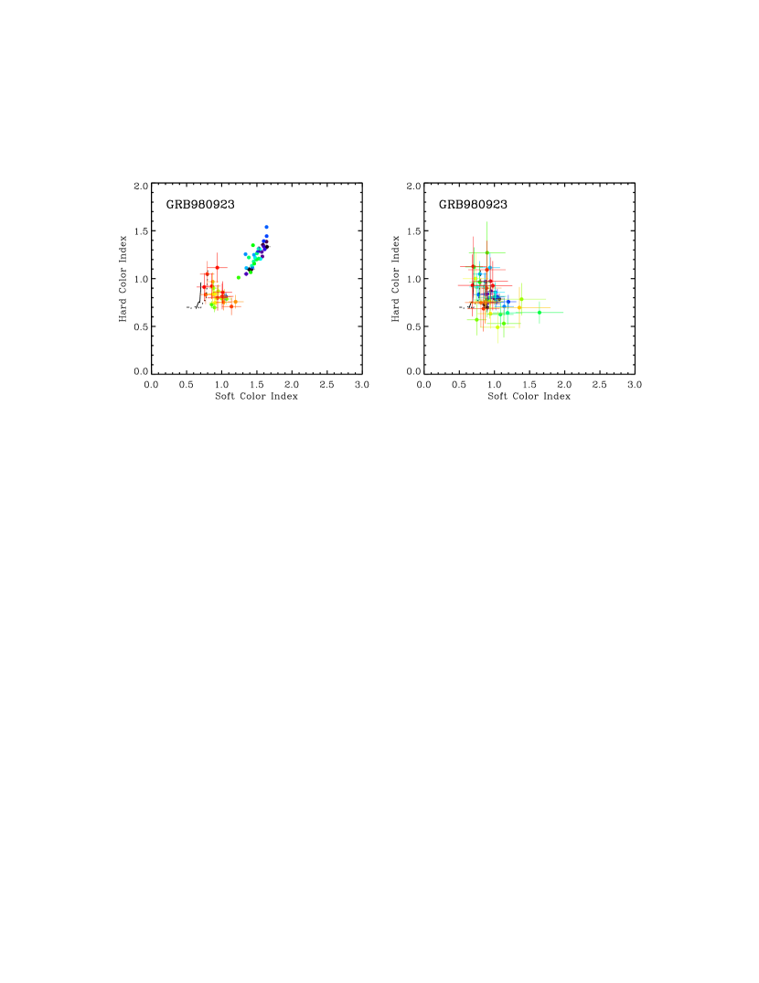
Figure 1.— Left panel: Color-color diagram of GRB980923 variability episode and tail emission (0-70 seconds). The crescent-like pattern is the variable emission while the decoupled cluster of points is the tail emission. Right panel: Color-color diagram of the tail emission only, covering a much longer time interval (40-100 seconds). Also plotted are the evolution patterns expected from the slow (solid) and fast-cooling (dashed) synchrotron spectrum.

Giblin et al. (1999a) have shown that the tail emission from GRB980923 resembles that of afterglow synchrotron emission due to an external shock. To illustrate the usefulness of the CCD technique, we show in Figure 5 the CCD for GRB980923. In this representation, the time evolution of the burst is preserved by a color sequence of the hardness ratios, with black/violet/blue signaling the onset of the burst and yellow/red signaling the end of the burst. The left panel shows the CCD for the time interval that brackets the entire burst (variability + tail). The variable emission of the burst shows a crescent-like pattern decoupled from a cluster of points that represent the tail of the burst.

The crescent pattern is typical among GRBs (Kouveliotou et al. 1993b , Giblin et al. 1999b ), however the clustering is less common. The crescent track exhibits a sawtoothing of soft-hard-soft evolution, indicative of the spectral behavior of the individual pulses that comprise the main burst emission. The pattern drastically changes when the variability ceases and the tail becomes visible. The tail cluster overlaps the region of the two-color plane that contains the evolution of the slow and fast-cooling synchrotron spectrum. This is best illustrated in the right panel of Figure 5, where the CCD is constructed from a longer time interval in the tail only. Unfortunately the CCD pattern of the tail is not completely resolved due to the increasingly large uncertainties in the hardness ratios that arise from the decreasing flux level. However, the points do lie in the correct region of the diagram. This decoupling of the points in the model-independent CCD is clear evidence for two distinct spectral components observed in a GRB.

Figure 6 shows the CCDs for the four fast-cooling candidates identified based on their spectral parameters in Table 2. The pattern for GRB920622 bears a striking resemblance to that of GRB980923 in the left panel of Figure 5. Like GRB980923, this burst contains a period of variability followed by a very smooth emission tail. The crescent pattern that arises from the variable part of the burst is clearly visible and spans nearly the same range of soft and hard color indices. However, the clear discontinuity between the burst emission and the tail emission in the CCD of GRB980923 is not as pronounced in the CCD of GRB920622. Nonetheless, the tail emission (denoted by the orange and red points) lies in the same region as those of GRB980923 and the synchrotron afterglow spectrum. The CCD pattern for GRB949419b (in the PF class) is similar, but appears more cluster-like in the region of synchrotron evolution.

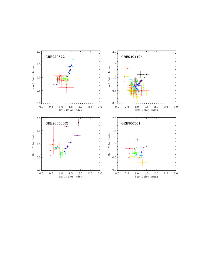
Figure 2.— Color-color diagrams for the four fast-cooling candidates from Table 3. Arrows indicate two-sigma upper limits.

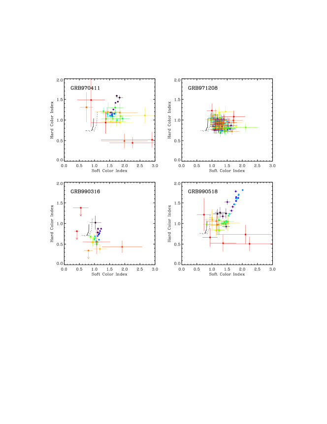
Figure 3.— Color-color diagrams for the marginal fast-cooling candidates from Table 3. Arrows indicate two-sigma upper limits.

Another burst of interest in the PF category is GRB960530. This event consists of two FREDs separated by $\sim 200$ seconds. The 2nd FRED only has about half of the peak intensity as the first. The CCD for the 2nd FRED is seen in Figure 6. The episode begins very hard on the rise and evolves through the synchrotron spectrum during the decay. Interestingly, although the 1st episode of GRB960530 is also a FRED, its color-color diagram (Figure 8) shows a broad crescent pattern that evolves much farther away from the synchrotron pattern. This may be a case where the external shock is clearly decoupled in time from the GRB.

The last event in Figure 6, GRB980301, shows an intriguing pattern that closely resembles the evolution pattern of the synchrotron spectrum. The evolution is mainly shaped like a reverse “L”, but marginally offset to higher soft color values and lower hard color values. In this case it is difficult to argue in favor or against the synchrotron model.

Figure 7 shows the CCDs of the four events from Table 3 that are only marginally consistent with fast-cooling. GRB970411 and GRB990518 show similar patterns that resemble those in Figure 6, but the consistency with the synchrotron pattern is weak. GRB971208 shows little evolution and a cluster of points partially overlapping the synchrotron region. GRB990316 shows a nearly identical pattern to that of GRB980301.

A total of 23 events from our sample showed CCDs inconsistent with the evolution of the synchrotron spectrum. Rather, most of these events showed the crescent pattern that are common among GRBs, as depicted in Figure 8. These events span a much larger range of hard and soft colors than expected from the synchrotron emission alone. Others were too weak to distinguish a pattern.

4. High-Energy Afterglow Candidates

We identify a total of 8 from our sample of 40 events as high-energy afterglow candidates based on their observed spectral parameters and color-color diagrams. Each burst is discussed in detail below.

4.0.1 GRB 910602

The observed spectral slope for GRB910602 is consistent with the spectral slope below $\nu_{\rm m}$ in the fast-cooling spectrum, although the slope below $\nu_{\rm c}$ in slow-cooling can not be ruled out, implying a value of $p=2$. A series of time-resolved fits with a uniform time resolution of 4.096 s revealed no softening of the spectrum, i.e, the slope remained constant with $\alpha_{p}\sim-0.5$ throughout the tail. Applying the relations in equation 6, for slow-cooling we expect $\beta=-0.78\pm 0.01$ and, from equations 4 and 5, for fast-cooling we expect $\beta=-4/7$ (radiative) or $\beta=-1/4$ (adiabatic). These values do not agree with the measured value $\beta=-1.74_{+0.11}^{-0.72}$. Although the spectrum appears to be consistent with that of the synchrotron spectrum, the evolution does not appear to be consistent with the evolution of a spherical blast wave.

4.0.2 GRB 920622

The time history of this burst bears a striking resemblance to that of GRB980923 reported by Giblin et al. (1999). Initially the burst is highly variable, then at $\sim 18$ s after the trigger time the burst enters a phase of smooth decay that lasts until $\sim 50$ s after the trigger. From Table 2, the time-integrated spectral fit suggests fast-cooling, with low-energy index $\alpha=-0.49\pm 0.04$. From the high-energy index, a value of $p=2.96\pm 0.26$ is inferred. The value of $\Delta=0.99\pm 0.26$ is marginally consistent (within two-sigma) with the expected value of 0.5 for slow-cooling. The time-integrated spectrum of the variable emission of the burst is in contrast with the fluence spectrum of the tail. The variable emission gives $\alpha_{\rm v}=-0.07\pm 0.01$, $\alpha_{\rm v}^{\prime}=-1.50\pm 0.04$, and $E_{{\rm v},b}=370\pm 12$ keV, suggestive of a spectral change near $\sim 18$ seconds. Note that the spectral parameters of the variable emission are not consistent with the synchrotron spectrum. We binned the tail emission into three time bins with S/N $\geq 45$ to model the spectral evolution, however the parameters were poorly constrained due to the steep nature of the flux decay. The spectral evolution of the variability + tail emission, however, can be seen in Figure 6. The tail of the burst appears consistent with the region of the diagram defined by the evolution of the synchrotron spectrum. The measured temporal index of the tail is $\beta\leq-2.98$, clearly inconsistent with the expected values for $\beta$ for $\nu<\nu_{\rm m}$. Interestingly, however, $\beta$ is nearly identical to the value of $p$ inferred from the high-energy slope, as expected for jet evolution.

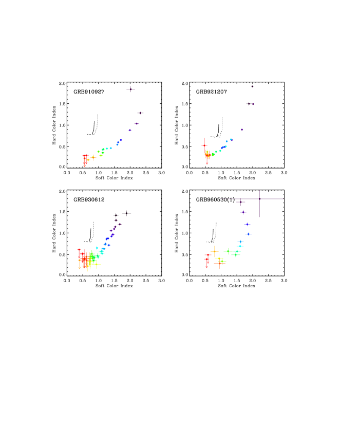
Figure 4.— A sample of color-color diagrams of GRBs that are not consistent with the evolution of the synchrotron spectrum. Arrows indicate two-sigma upper limits.

4.0.3 GRB 940419b

The smooth rise and decay structure of this burst place it in the PF category. Like the tail emission of GRB920622, this burst also shows a low-energy slope consistent with the fast-cooling spectral slope below $\nu_{\rm m}$. The measured temporal slope is $\beta\leq-1.75$. While this slope is not consistent with the temporal index below $\nu_{\rm m}$, it is consistent with the expected values of $\beta=-2.56\pm 0.55$ (radiative) and $\beta=-1.95\pm 0.55$ (adiabatic) for $\nu>\nu_{\rm m}$, given the large uncertainties. We further binned the data in the tail to S/N $\geq 45$ and constrained the evolution of the break energy by holding the low and high-energy spectral indices fixed to their values derived from the time-integrated fit. We find $E_{b}\sim(t-t_{0})^{-1.21\pm 0.15}$ for $t_{0}$ fixed at $-25.0$ s ($\chi^{2}/d.o.f.=7.52/8$). Additional fits with other larger values of $t_{0}$ gave slightly shallower indices, as expected if one compares the behavior to that of $\beta$ and $t_{0}$. For an adiabatic fast-cooling spherical blast-wave we expect the break energy to decay as $-1.5$, within two-sigma of our measured value. As seen from the CCD in Figure 5, the spectral evolution of this burst is very close to that of the synchrotron spectrum, although the rise of the burst tends to be somewhat harder in the soft color index than expected from evolution of the synchrotron spectrum alone.

4.0.4 GRB 960530

GRB960530 is of particular interest because of its striking temporal behavior. The burst has two distinct episodes of emission, each having a FRED-like time profile. The second episode, much weaker with a peak intensity less than half of the first, occurs $\sim 200$ seconds after the first. As seen in Table 2, the low-energy slope of the second episode is consistent with the fast-cooling slope below $\nu_{\rm m}$, however the value of $p=3.76\pm 0.37$ is large mainly because the high-energy slope is not well-constrained. The value of $p$ derived for the first episode is not unreasonable, however the low-energy slope is roughly three-sigma away from the expected value of $-0.5$. The decay index for the second episode is $\beta\leq-2.13$, not inconsistent with the expected values $\beta=-4.57\pm 1.57$ and $\beta=-3.75\pm 1.57$ for radiative and adiabatic fast-cooling, respectively. The CCD of the second emission episode of this burst (Figure 6) indicates that during the decay the emission evolves into the synchrotron spectrum.

4.0.5 GRB 970411

From Table 2, the low-energy index of this burst is nearly four-sigma from the value $-0.5$ expected in the fast-cooling regime. However, it does have $p=2.2\pm 0.08$, consistent with typical afterglow values and particle acceleration models of relativistic shocks (e.g., Gallant et al. (2000)). Additionally, the change in slope, $\Delta$ is less than three-sigma from the expected value of $-0.5$ for the cooling break in the slow-cooling regime. For slow-cooling, we expect the temporal slope to be $\beta=-0.53\pm 0.04$ for $\nu<\nu_{\rm c}$ and $\beta=-1.15\pm 0.08$ for $\nu>\nu_{\rm c}$. For $\nu>\nu_{\rm m}$ in fast-cooling we expect $\beta=-1.60\pm 0.08$ (radiative) and $\beta=-1.15\pm 0.08$ (adiabatic). Our measured value of the decay, $\beta=-2.06_{+0.20}^{-0.21}$, is marginally consistent (within two-sigma) with the radiative fast-cooling slope. More notably, it is consistent (within one-sigma) with the value of $p$. A series of spectral fits during the tail of the burst holding the low and high-energy spectral indices constant show that $E_{b}$ decays with time described by a power-law of the form $E_{b}\sim(t-t_{0})^{-0.96\pm 0.26}$ for $t_{0}=16$ s ($\chi^{2}/d.o.f.=4.02/3)$, marginally consistent with the adiabatic evolution (spherical or jet) of $\nu_{\rm m}$.

4.0.6 GRB 971208

GRB971208 is the longest burst ever detected with BATSE. The temporal structure of the burst is a simple smooth FRED lasting several thousand seconds. The emission is soft, with no emission in channel 4 ($E>300$ keV). The spectral parameters tend to favor fast-cooling, but not strongly, as the value of $p=4.06\pm 0.04$ is unusually high. The value of $\Delta=1.48\pm 0.04$ is well-determined, and very far from the value expected for slow-cooling ($\Delta=0.5$). Although in apparent contradiction to this, the CCD pattern for this event (Figure 7) shows a strong resemblance to that of the tail of GRB9890923 in Figure 5.

4.0.7 GRB 980301

GRB980301 shows a low-energy slope consistent with fast-cooling but also a value of $p=2.48\pm 0.13$, remarkably consistent with values of observed afterglows. The change in slope across the break energy is slightly higher than that expected for slow cooling (but within two-sigma). If the spectrum is fast-cooling, then we expect $\Delta=0.74\pm 0.13$, based on the measured high-energy slope. This value is within one-sigma of the value $\Delta=0.69\pm 0.13$ that we derive from the measured slopes. For radiative evolution we expect $\beta=-1.84\pm 0.13$, while for adiabatic evolution we expect $\beta=-1.36\pm 0.13$. However, we measure a much steeper value of $\beta=-2.50_{+0.05}^{-1.58}$, suggesting an evolution inconsistent with the hydrodynamics of a spherical blast wave, but consistent with that of a jet. The CCD pattern for GRB980301 is shown in Figure 6. Although very similar to the model pattern, the observed pattern appears to be displaced.

4.0.8 GRB 981203

The measured low and high-energy spectral indices for this event are notably different than those of other bursts listed in Table 2. The low-energy spectral index is consistent with the spectral slope below $\nu_{\rm m}$ in the slow-cooling mode and below $\nu_{\rm c}$ in the fast-cooling regime. Interestingly, for the fast-cooling regime the high-energy index is marginally consistent with the spectral slope for $\nu_{\rm c}<\nu<\nu_{\rm m}$. The direct implication here is that $\nu_{\rm m}$ is above the BATSE window and has yet to evolve through. Hence the value of $p$ is undetermined. The flux in the tail was too weak to follow the evolution of the spectrum with any reasonable accuracy. From equation 3 and 4, clearly the temporal decay should be very shallow, unlike our measured value of $\beta=-1.61_{+0.002}^{-0.013}$. This evolution is not consistent with the evolution of a spherical blast wave into a constant density medium.

5. Discussion

The diverse temporal and spectral properties of GRBs leave their origin open to different interpretations. From our analysis, we have identified a subset of gamma-ray bursts that exhibit smooth high-energy ($\sim$ 25-300 keV) decay emission whose spectral properties are very similar to that of fast-cooling synchrotron emission that results from a power-law distribution of relativistic electrons accelerated in a forward external shock. The 25-300 keV time histories of the high-energy afterglow candidates are shown in Figure 9. The diversity of the time profiles suggests that the GRB time history is not necessarily the distinguishing feature of external shock emission in the fireball model. The diversity also suggests that the afterglow may be disconnected from the burst emission (e.g., GRB960530), or overlap the burst emission (e.g., GRB920622). BeppoSAX has demonstrated the existence of both cases: overlap or continuation of the afterglow onset with the prompt burst emission [e.g., GRB970508 (Piro et al. (1998)), and more recently GRB990510 (Pian et al. (2001))], and the case in which the afterglow begins at a later time, disconnected from the prompt GRB [e.g., GRB970228 (Costa et al. (2000))]. Our analysis further suggests that in some cases (e.g., GRB971208) the early high-energy afterglow may actually be the burst emission itself. This situation could arise if the energy deposition in the internal shocks is too low.

Figure 5.— Time histories (25-300 keV) for the eight high-energy afterglow candidates.

The spectra of a significant fraction of bursts in our sample, however, show inconsistencies with the synchrotron model. From a catalog of BATSE GRB spectra, we see that the low and high-energy spectral indices follow well-defined distributions (Preece et al. (2000)). For example, the distribution of low-energy power-law indices given in Figure 7 of Preece et al. (2000) peaks near $\alpha_{\rm low}\sim-1$. Roughly $\sim 200$ of the 5500 spectra in the distribution are consistent with the expected value of $\alpha_{\rm low}$ below $\nu_{\rm m}$, or about $\sim 4\%$. If we adopt the hypothesis that GRB spectra are not synchrotron spectra, then on average $\sim 4\%$ of the time we expect to measure parameters consistent with the synchrotron spectrum purely by chance coincidence. This implies that we can expect $\sim 0.8$ events from Table 2 to have $\alpha_{\rm low}=-1.5$ ($\alpha=-0.5$) purely by chance. Clearly, our total of eight candidate events exceeds this limit. These events are thus likely sources of synchrotron emission.

Table 4Jet Candidates

GRB	Trigger	$p$	$\beta$
910602	257	$2.00\pm 0.01$	$1.74_{-0.11}^{+0.72}$
920622	1663	$2.96\pm 0.26$	$>2.98$
920813	1807	$2.02\pm 0.02$	$2.10_{-0.04}^{+6.05}$
970302	6111	$1.46\pm 0.10$	$1.49_{-0.11}^{+0.93}$
970411	6168	$2.20\pm 0.08$	$2.06_{-0.20}^{+0.21}$
980301	6621	$2.48\pm 0.13$	$2.50_{-0.05}^{+1.58}$
990316	7475	$3.04\pm 0.09$	$>2.20$
990322	7488	$0.84\pm 0.06$	$0.87_{-0.01}^{+0.02}$
990415	7520	$2.56\pm 0.16$	$>2.23$
Pre-break Jet Candidates
910131	2151	$1.78\pm 0.11$	$0.71_{-0.11}^{+0.31}$
940419b	2939	$3.32\pm 0.55$	$>1.75$
960530	5478	$2.96\pm 0.22$	$1.49_{-0.04}^{+0.77}$
970925	6397	$2.56\pm 0.13$	$1.98_{-0.21}^{+0.31}$
971208	6526	$4.06\pm 0.04$	$1.34_{-0.01}^{+0.11}$

Recent studies on electron acceleration models for ultra-relativistic shocks predict values of the electron index in a narrow range $2.0\leq p\leq 2.5$ (Gallant et al. (1999), Gallant et al. (2000)). Our values maintain a significant dispersion under the assumption that the observed high-energy afterglow is equivalent to the high-energy slope of the fast or slow-cooling synchrotron spectrum (i.e., $\alpha_{\rm high}+1=-p/2$). Electron indices in Table 2 tend to be steepr on average than $p=2.5$. One possible alternative for a high value of $p$ ($p\simeq 3$) may be due to a shock generated in a decreasing density, $n\propto r^{-2}$, external medium that is the result of a massive stellar wind (Chevalier (1998), Chevalier et al. (1999)). On the other hand, Sari (2000) pointed out that there is no reason why the value of $p$ should be different for wind models. Note that several values of $p$ in Table 3 are below $p=2$. Hard electron indices ($1<p<2$) have recently been reported for the jet model of GRB00301c (Panaitescu (2001)) assuming a broken power-law electron energy distribution. Similarly, a jet interpretation for GRB010222 would also require a flatter electron index, based on analysis of the BeppoSAX data (In’T Zand et al. (2001)). However, In’T Zand et al. (2001) show that the slowing of the ejecta into the non-relativistic regime yields $p=2.2$. From a theory viewpoint, Malkov (1999) has shown that it is possible to obtain a hard electron electron distribution in Fermi acceleration models. While the model predictions for the range of electron indices appear somewhat uncertain, the observed dispersion in $p$ values may be strongly linked to the accuracy of the fitted value of $\alpha_{\rm high}$. Systematic effects may play a role that introduces a bias toward steeper values in the estimation of the high-energy power-law index.

Our analysis shows that the tail temporal decays are well-described by a power-law with a mean index $\langle\beta\rangle=-2.03\pm 0.51$. While the spectral parameters of approximately $20\%$ of the decays in our sample are in generally good agreement with the synchrotron spectrum, the temporal evolution, in general, does not agree well with the evolution of a spherical blast wave in a homogeneous medium. There are alternatives that might explain this deviation: first, we only considered fully radiative or fully adiabatic evolution. More than likely the fireball is neither fully radiative nor fully adiabatic throughout its evolution, although at the very early stages the evolution may nearly be fully radiative while at latter stages the evolution is completely adiabatic. Böttcher and Dermer (2000) have considered the early afterglow regime with the intermediate cases: partially radiative or partially adiabatic blast waves. They find that the temporal decay of the spectral flux in the fast-cooling regime is a function of $\epsilon=\epsilon_{e}\epsilon_{\rm rad}$, where $\epsilon_{\rm rad}$ is the fraction of energy radiated by the accelerated electrons, or $F_{\nu}\propto\nu^{-1/2}t^{-2{(1+\epsilon)\over(8-\epsilon)}}$ for $\nu_{\rm c}<\nu<\nu_{\rm m}$ and $F_{\nu}\propto\nu^{-p/2}t^{-{{2(1+\epsilon)+6(p-1)}\over{(8-\epsilon)}}}$ for $\nu>\nu_{\rm m}$. Higher efficiencies therefore produce steeper temporal slopes. However, as can be seen for $\epsilon=0.8$, we obtain $F_{\nu}\propto\nu^{-1/2}t^{-1/2}$ for $\nu_{\rm c}<\nu<\nu_{\rm m}$. This is steeper than the expected value of $-1/4$ from equation 4 but not steep enough to match the discrepancies in our observations.

Another possibility to consider is a jet-like geometry or collimated outflow, as opposed to the simple spherical blast wave. The break in the light curve may occur at early times after the initial shock, as in the case of GRB980519, where evidence exists for a break to a steep decay that apparently occurred during the few hours between the GRB and the first afterglow detection (Sari et al. (1999)). Rhoads (1999) has shown for adiabatic evolution that the time of the break in the observer’s frame goes as $t_{b}\propto\theta_{c}^{2}$. A very early break therefore requires a very small $\theta_{c}$. If $\theta_{c}<\theta_{b}$ initially, then the slope is steep from the start. This implies one of two possiblities: (1) very narrow emission spots, or “nuggets”, within a narrow collimation angle, or (2) a very small value of $\Gamma$ such that $\Gamma^{-1}>\theta_{c}$. The second option is not likely since the observed emission is in the keV to MeV range and $\nu_{\rm m}\propto\Gamma^{4}$, requiring a high Lorentz factor. A list of events from Table 2 and 3 with comparable electron indices and temporal indices (as required for a jet-like blast-wave) are presented in Table 4. Note that although the value of $p$ for GRB990322 is low, the temporal decay does follow the $t^{-p}$ relation. Events with values of $\beta$ shallower than $p$ may be events in which the break occurs at some later time after the GRB. We categorize these events as pre-break jet candidates. Three of these events (GRB940419b, GRB960530, and GRB970925) have some spectral properties characteristic of the synchrotron spectrum (see last column of Table 2). The five bursts labeled in Figure 3 are also candidates for jet outflows. More importantly, note that three of these events (GRB920622, GRB980301, and GRB970411) are strong candidates because they belong to the group of high-energy afterglow candidates presented in $\S 4$ that were selected based on their spectral properties. The spectra of the remaining two events (GRB920801 and GRB931223) are only marginally consistent with synchrotron emission from an external shock.

6. Summary and Conclusion

Our temporal and spectral analysis of the smooth extended gamma-ray decay emission in GRBs has shown evidence of signatures for early high-energy afterglow emission in gamma-ray bursts. The extended decay emission is best described with a power-law function $F_{\nu}\propto t^{\beta}$ rather than an exponential, similar to the results of Ryde and Svensson (2001) who studied the decay phase of a sample of GRB pulses with a broad range of durations. From our sample of 40 events, we find $\langle\beta\rangle\approx-2$ for long, smooth decays. Color-color diagrams have provided a qualitative interpretation of the burst spectral evolution and allow a simple comparison with the evolution expected from the synchrotron model as well as comparison of spectral evolution among GRBs. The CCD patterns and the spectral analysis indicate that $\sim 20\%$ of the events in our sample are consistent with synchrotron emission expected from an external shock. Interestingly, three of these events have decay rates consistent with that expected from the evolution of a jet, $F_{\nu}\sim t^{-p}$. Because the break is essentially at the onset of deceleration, the jet must, at least, be very narrow, since $\theta_{c}<1/\Gamma$. Table 4 suggests that in some cases the break occurs at a later time, so that the prompt emission we observe is pre-break, $\theta_{c}>1/\Gamma$ and consistent with spherical geometry. A possible scenario is one in which the ejecta is very grainy, where the nuggets in the ejecta are smaller than $1/\Gamma$, similar to the model discussed by Heinz and Begelman (1999). Huang et al. (1999) (see also Wei and Lu 2000) have shown that the break in the light curve is more of a smooth transition due to the off-axis emission of a jet with no angular dependence. The steep light curve can only occur if the angular size of the nugget is less than $1/\Gamma$.

Connaughton (2001) has investigated the average late-time temporal properties of GRBs observed with BATSE and found statistically significant late time power-law decay emission that softens relative to the initial burst emission, suggesting the existence of early high-energy afterglow. Other studies using PHEBUS (Tkachenko et al. (2000)) and APEX (Litvine et al. (2000)) bursts show similar behaviors in late-time GRB light curves. Collectively, these studies strongly suggest that the afterglow emission may overlap or be connected to the prompt, variable burst emission. On the other hand, it is clear that not all GRBs exhibit such behavior. In some cases, the initial gamma-ray flux from the external shock may simply be too low to detect (e.g., see Figure 4 in Giblin et al. 2000). In other cases, the bulk Lorentz factor may be too low to generate the gamma-ray photons upon impact with the surrounding medium.

As the number of afterglow/counterpart detections increases, the relationship of the afterglow emission to the gamma-rays released in the initial phase of the burst can be studied systematically. The capabilities of Swift (Gehrels (2002)) will allow broad spectral coverage using three co-aligned instruments (BAT, XRT, and UVOT) during the gamma-ray phase and early afterglow phase of the burst and facilitate the distinction between the GRB and the onset of the afterglow based on temporal and spectral information. With well-constrained spectral and temporal parameters in hand, plots of temporal index vs. spectral index can be readily constructed and thus provide information on the geometry of the fireball and definitively test the internal/external shock model for GRBs.

References

- Akerlof et al. (1999) Akerlof, C. W., Balsano, R., Barthelmy, S., et al., 1999, Nature, 398, 400
- Band et al. (1993) Band, D., Matteson, J., Ford, L., et al., 1993 ApJ, 413, 281
- Beloborodov (2000) Beloborodov, A. M., 2000, ApJ, 539, L25
- Bloom et al. (1998) Bloom, J. S, Frail, D. A., Kulkarni, S. R., et al., 1998, ApJ, 508, L21
- Böttcher and Dermer (2000) Böttcher, M., and Dermer, C. D., 2000, ApJ, 532, 281
- Briggs et al. (1999) Briggs, M., S., Band, D., Kippen, R. M., et al., 1999, ApJ, 524, 82
- Burenin et al. (1999) Burenin, R., A., Vikhlinin, A. A., Terekhov, O. V., et al., 1999, A & AS, 138, 443
- Chevalier (1998) Chevalier, R., 1998, ApJ, 499, 810
- Chevalier et al. (1999) Chevalier, R., and Li, Z. Y., 1999, ApJ, 520, L29
- Connaughton et al. (2001) Connaughton, V., 2001, ApJ, submitted.
- Costa et al. (2000) Costa, E.,, 2000, in Gamma-Ray Bursts: 5th Huntsville Symposium, eds. Kippen, R. M., Mallozzi, R. M. (AIP Conference Proceedings: New York), pp. 365.
- Dermer and Mitman (1999) Dermer, C. D., and Mitman, K. E., 1999, ApJ, 513, L5
- Fishman et al. (1989) Fishman, G. J., et al. 1989, in Gamma-Ray Observatory Science Workshop, NASA/GSFC Greenbelt, MD, ed. W. N. Johnson, pp. 2.
- Ford et al. (1995) Ford, L., Band, D. L., Matteson, J. L., et al., 1995, ApJ, 439, 307
- Fruchter et al. (1999) Fruchter, A., et al., 1999, ApJ, 519, L13
- Galama et al. (1998) Galama, T., J., et al., 1998, ApJ, 500, L97
- Galama et al. (1999) Galama, T., J., et al., 1999, Nature, 398, 394
- Gallant et al. (1999) Gallant, Y. A., Achterberg, A., and Kirk, J. G., 1999, A&AS, 138, 549
- Gallant et al. (2000) Gallant, Y. A., Achterberg, A., and Kirk, J. G., and Guthmann, A., 2000, in Gamma-Ray Bursts: 5th Huntsville Symposium, eds. Kippen, R. M., Mallozzi, R. M. (AIP Conference Proceedings: New York), pp. 524.
- Gehrels (2002) Gehrels, N., 2002, in Gamma-Ray Bursts and Afterglow Astronomy 2001, ed. Ricker, G. (AIP Conference Proceedings: New York), in press.
- (21) Giblin, T., W., van Paradijs, J., Kouveliotou, C., et al., 1999, ApJ, 524, L47
- (22) Giblin, T., W., Kouveliotou, C., van Paradijs, J., et al., 1999, BAAS, 193, 79.06
- Giblin et al. (2000) Giblin, T., W., et al. 2000, in Gamma-Ray Bursts: 5th Huntsville Symposium, eds. Kippen, R. M., Mallozzi, R. M. (AIP Conference Proceedings: New York), pp. 394.
- Granot and Sari (2001) Granot, J., and Sari, R., 2001, ApJsubmitted, [astro-ph/0108027]
- Huang et al. (1999) Huang, Y. F., Dai, Z. G., and Lu, T., 1999, MNRAS, 309, 513
- In’T Zand et al. (1999) In’T Zand, J. J. M., et al. 1999, ApJ, 516, L57
- In’T Zand et al. (2001) In’T Zand, J. J. M., et al. 2001, ApJ, 559, 710
- Kobayashi et al. (1997) Kobayashi, S., Piran, T., and Sari, R., 1997, ApJ, 490, 92
- Kouveliotou et al. (1992) Kouveliotou, C., Paciesas, W. S., Fishman, G. J., et al., 1992, Proceedings of the Compton Observatory Science Workshop, NASA ref. Publication, pp. 61.
- (30) Kouveliotou, C., Meegan, C. M., Fishman, G. J., et al., 1993, ApJ, 413, L101
- (31) Kouveliotou, C., Paciesas, W. S., Fishman, G. J., et al., 1993, A & AS, 97, 55
- Litvine et al. (2000) Litvine, D. A., et al. 2000, in Gamma-Ray Bursts: 5th Huntsville Symposium, eds. Kippen, R. M., Mallozzi, R. M. (AIP Conference Proceedings: New York), pp. 390.
- Malkov (1999) Malkov, M., 1999, ApJ, 511, L53
- Mészáros and Rees (1992) Mészáros, P., and Rees, M. J., 1992, MNRAS, 258, 41
- Mészáros and Rees (1997) Mészáros, P., and Rees, M. J., 1997, ApJ, 476, 232
- Mészáros and Rees (1999) Mészáros, P., and Rees, M. J., 1999, MNRAS, 306, L39
- Panaitescu (2001) Panaitescu, A., 2001, ApJ, 556, 1002
- Pian et al. (2001) Pian, E., et al. 2001, A & A, 372, 456
- Piran (1999) Piran, S., 1999, Physics Reports, 314, 575
- Piro et al. (1998) Piro, L., 1998, A & A, 331, L41
- Preece et al. (1998) Preece, R. D., Pendleton, G. N., Briggs, M. S., et al., 1998, ApJ, 496, 849
- Preece et al. (2000) Preece, R. D., Briggs, M. S., Mallozzi, R. S., et al., 2000, ApJS, 126, 19
- Press et al. (1992) Press, W. H., Teukolsky, S. A., Vetterling, W. T., and Flannery, B. P., 1992, Numerical Recipes in C, (Cambridge University press: New York), p. 697.
- Rhoads (1999) Rhoads, J. E., 1999, ApJ, 525, 737
- (45) Ryde, F. and Svensson, R., 2001, Gamma-Ray Bursts in the Afterglow Era: 2nd Workshop, in press.
- Sari et al. (1996) Sari, R., Narayan, R., and Piran, T., 1996, ApJ, 473, 204
- Sari and Piran (1997) Sari, R., and Piran, T., 1997, ApJ, 485, 270
- Sari et al. (1998) Sari, R., Piran, T., and Narayan, R., 1998, ApJ, 497, L17
- Sari and Piran (1999) Sari, R., and Piran, T., 1999, ApJ, 520, 641
- Sari et al. (1999) Sari, R., Piran, T., and Halpern, J. P., 1999, ApJ, 519, L17
- Sari (2000) Sari, R., 2000, in Gamma-Ray Bursts: 5th Huntsville Symposium, eds. Kippen, R. M., Mallozzi, R. M. (AIP Conference Proceedings: New York), pp. 504.
- Schaefer and Dyson (1995) Schaefer, B. E., and Dyson, S. E., 1995, in Gamma-Ray Bursts: 3rd Huntsville Symposium, eds. Kouveliotou, C. K., Briggs, M. S., Fishman, G. J., (AIP Conference Proceedings 384: New York), pp. 96.
- Tkachenko et al. (2000) Tkachenko, A. Y., et al. 2000, A & A, 358, L41
- Vietri (1997) Vietri, M., 1997, ApJ, 488, L105
- Vietri (2000) Vietri, M., 2000, Astroparticle Physics, 14, 211
- Vreeswijk et al. (1999) Vreeswijk, P. M., Galama, T. J., Owens, A., et al., 1999, ApJ, 523, 171
- Waxman (1997) Waxman, E., 1997, ApJ, 489, L33
- Wijers, Rees, and Mészáros (1997) Wijers, R., Rees, M., and Mészáros, P., 1997, MNRAS, 288, L51