SUSX-TH/02-004 NORDITA-2002-2 AP

MHD inverse cascade in the early Universe

Mark Hindmarsh

Centre for Theoretical Physics, University of Sussex, Brighton BN1 9QJ, U.K.

and

M. Christensson, A. Brandenburg

Nordita, Blegdamsvej 17, DK-2100 Copenhagen Ø, Denmark

We have carried out numerical simulations of freely decaying magnetohydrodynamic (MHD) turbulence in three dimensions, which can be applied to the evolution of stochastic magnetic fields in the early Universe. For helical magnetic fields an inverse cascade effect is observed in which magnetic helicity and energy is transfered from smaller scales to larger scales, accompanied by power law growth in the characteristic length scale of the magnetic field. The magnetic field quickly reaches a scaling regime with self-similar evolution, and power law behaviour at high wavenumbers. We also find power law decay in the magnetic and kinematic energies.

PRESENTED AT

COSMO-01
Rovaniemi, Finland,
August 29 – September 4, 2001

1 Introduction

Magnetic fields are ubiquitous in the Universe, being observed in nature on scales from planetary size to galaxy cluster size [2, 3]. In galaxies and galaxy clusters, the typical strength is of order a few $\mu$Gauss, which is thought to be produced by dynamo action on a seed field. In galaxies the dynamo timescale is roughly a rotation period, $10^{8}$ Yr, and a simple calculation [2] based on the age of a typical galaxy shows that the seed field must have been about $10^{-20}$ Gauss, or perhaps less in the currently favoured models with a cosmological term [5].

There is no shortage of ideas for generating this seed field. The more conventional astrophysical explanations are based on a Biermann battery operating at the era of reionisation (see e.g. [6] and the references therein). There are more speculative ideas based on various models of inflation [7], phase transitions [8] and primordial black holes [9].

All these mechanisms have the common feature of producing stochastic, homogeneous and isotropic magnetic and velocity fields which can be characterised by their power spectra and characteristic initial scales. Our interest here is to try and make model-independent statements about the evolution of the magnetic fields once they are generated. This article, which is based on Ref. [10], studies the evolution of a stochastic magnetic field generated at a phase transition, such as the confinement transition in QCD at $t\simeq 1$ sec, or the electroweak symmetry-breaking transition at $t\simeq 10^{-11}$ sec. It therefore falls into the category of decaying 3D MHD turbulence, which has been studied before in the MHD community [11, 12, 13, 14, 15, 16]. Most directly comparable to our work, Biskamp and Müller [15] studied the energy decay in incompressible 3D magnetohydrodynamic turbulence in numerical simulations at relatively high Reynolds number, and in a companion letter [16] studied the scaling properties of the energy power spectrum.

We focus here on the transfer of magnetic energy from small to large scales, as necessitated by the conservation of magnetic helicity. This is important for a primordial magnetic field to reach a large enough scale with sufficient amplitude to be relevant for seeding the galactic dynamo [17].

We perform 3D simulations both with and without magnetic helicity, starting from statistically homogeneous and isotropic random initial conditions, with power spectra suggested by cosmological applications. We find a strong inverse cascade in the helical case, with the coherence scale of the field growing as $t^{0.5}$, and equivocal evidence for a weak cascade when only helicity fluctuations are present. In the helical case we also find a self-similar power spectrum with an approximately $k^{-2.5}$ behaviour at high $k$. We find decay laws for the magnetic and kinetic energies of $t^{-0.7}$ and $t^{-1.1}$, respectively, in the helical case, and $t^{-1.1}$ for both in the non-helical case.

2 Evolution of magnetic fields in the early Universe

A convenient benchmark is to assume that the field is created on the horizon scale with a power spectrum $k^{n}$, taking all the energy in the Universe, and that it is subsequently completely frozen into the plasma [17]. If one takes the epoch of creation to be either the QCD transition or the electroweak transition, one finds that the RMS fluctuations on the scale of a protogalaxy are roughly

$$B(t_{0},L=0.5\mathrm{Mpc})<\left\{\begin{array}[]{ll}10^{-14-3n}\;{\textrm{G}}&\mathrm{QCD}\\[-2.0pt] 10^{-20-4.5n}\;{\textrm{G}}&\mathrm{EW}\end{array}\right.$$

Thus we see that for causal fields ($n\geq 2$) there needs to be some amplification on large scales for there to be any interesting seed field for the galactic dynamo.

In fact, the field is not strictly frozen into the plasma, and in order to calculate observable effects, we must determine how the field scale length $\xi$ and magnetic energy $E_{M}$ evolves. There are various scaling arguments which have been put forward: for example, for ideal MHD (infinite conductivity) and with no helicity Olesen [18] (and later Son [19], Field and Carroll [20] and Shiromizu [21]) argued

$$\xi(t)\sim t^{2/(n+5)},$$ (1)

where $t$ is conformal time. The effect of having a conserved helicity modifies this scaling law to [4, 20, 19]

$$\xi(t)\sim t^{2/3},\qquad E_{M}\sim t^{-2/3}.$$ (2)

Early numerical experiments with a shell model of the full MHD equations [22] suggested $\xi\sim t^{0.25}$, and focussed attention on the possibility of an inverse cascade, in which power is transferred locally in $k$-space from small to large scales.

3 MHD equations

The MHD equations in an expanding Universe are most conveniently expressed in terms of conformally rescaled fields ${\mathbf{B}}$, ${\mathbf{u}}$ and dissipation parameters $\nu$, $\eta$, and in the gauge $A^{0}=\eta\mbox{\boldmath$\nabla$}\mbox{\boldmath$\cdot$}{\mathbf{u}}$ [23, 10].

The matter and radiation in the early Universe is modelled as an isothermal compressible gas with a magnetic field, which is governed by the momentum equation, the continuity equation, and the induction equation, written here in the form

$$\frac{\partial{\mathbf{u}}}{\partial t} = -{\mathbf{u}}\cdot\mbox{\boldmath$\nabla$}{\mathbf{u}}-c_{s}^{2}\mbox{\boldmath$\nabla$}\ln\rho+\frac{{\mathbf{J}}\times{\mathbf{B}}}{\rho}+\frac{\mu}{\rho}\left(\nabla^{2}{\mathbf{u}}+\frac{1}{3}\mbox{\boldmath$\nabla$}\mbox{\boldmath$\nabla$}\cdot{\mathbf{u}}\right),$$ (3)

$$\frac{\partial\ln\rho}{\partial t} = -{\mathbf{u}}\cdot\mbox{\boldmath$\nabla$}\ln\rho-\mbox{\boldmath$\nabla$}\cdot{\mathbf{u}},$$ (4)

$$\frac{\partial{\mathbf{A}}}{\partial t} = {\mathbf{u}}\times{\mathbf{B}}+\eta\nabla^{2}{\mathbf{A}},$$ (5)

where ${\mathbf{B}}=\nabla\times{\mathbf{A}}$ is the magnetic field in terms of the magnetic vector potential ${\mathbf{A}}$, ${\mathbf{u}}$ is the velocity, ${\mathbf{J}}$ is the current density, $\rho$ is the density, $\mu$ is the dynamical viscosity, and $\eta$ is the magnetic diffusivity.

In the ideal limit $\mu=\eta=0$, there is a conserved quantity in addition to the energy, which is the magnetic helicity $H_{\rm M}$, given by

$$H_{\rm M}=\int{\mathbf{A}}\cdot{\mathbf{B}}\,d^{3}x.$$ (6)

Helicity is known to be important in dynamo theory [24, 25], where turbulence is driven. We shall also be able to confirm its importance in decaying turbulence.

An important dynamical quantity is the magnetic Reynolds number $Re_{\rm M}=Lv/\eta$, where $L$ and $v$ are the typical length scale and velocity of the system under consideration, because it measures the importance of the non-linear term in the equation for the magnetic field. In the early Universe, $Re_{\rm M}$ can be very large. This is often taken to mean that the magnetic field is frozen into the plasma, and the scale length of the field increases only with the expansion of the Universe. This is in general untrue, because turbulence can transfer energy to different length scales [22]. Not only can there be the usual direct cascade of energy from large to small scales, but also an inverse cascade, increasing the overall comoving correlation length [24].

4 Plasma properties in the early Universe

We are considering the time before recombination, when the plasma in the early Universe has a relativistic equation of state $p=\rho/3$, and therefore a sound speed $c_{s}=1/\sqrt{3}$. The number species contributing to the pressure gradually decreases with the temperature $T$, until $T\simeq m_{e}$, the electron mass, when only photons and neutrinos remain relativistic. At that point the number of charge carriers in the plasma reduces by a very large factor: for $T\gg m_{e}$, the electron number density $n_{e}$ is approximately equal to the photon number density $n_{\gamma}$, while for $T\ll m_{e}$ $n_{e}/n_{\gamma}=n_{B}/n_{\gamma}\simeq 10^{-10}$, where $n_{B}$ is the baryon number density.

The transport properties of the plasma are determined from the mean free path $l_{\rm mfp}$ of the relevant particles involved in the transport of the quantity of interest, which typically is $l_{\rm mfp}\sim 1/\alpha|\log\alpha|T$ [26], where $\alpha$ is the fine structure constant. From this we can infer that the conductivity is

$$\sigma\sim\left\{\begin{array}[]{ll}T/\alpha|\log\alpha|&T\gg m_{e}\\ (n_{e}/n_{\gamma})(m_{e}^{2}/T)/\alpha&T\ll m_{e}\\ \chi(n_{B}/n_{\gamma})(T/m_{e})^{2}Te^{-2}&T<T_{\mathrm{dec}}\end{array}\right.,$$ (7)

where $T_{\mathrm{dec}}$ is the temperature at photon decoupling, roughly 1 eV.

The viscosity parameter $\nu$ is given by

$$\nu\equiv\eta/\rho\sim\left\{\begin{array}[]{ll}1/\alpha^{2}|\log\alpha|T&T\gg m_{e}\\ (n_{\gamma}/n_{e})(m_{e}^{2}/T^{2})/\alpha T&T\ll m_{e}\end{array}\right.$$ (8)

We can estimate the importance of non-linear terms relative to diffusion from the Reynolds numbers of the plasma, the hydrodynamical $\mathrm{Re}=vL/\nu$ and magnetic $\mathrm{Re}_{M}=vL\sigma$. Upper bounds are obtained by assumed a fluid flowing at the speed of light on a scale somewhere between the mean free path and the particle horizon $ct$:

$$(\alpha,1/\alpha^{2}\log^{2}\alpha)\mathrel{\mathchoice{\lower 0.5pt\vbox{\halign{$\math\displaystyle\hfil#\hfil$\cr\scriptstyle<\crcr{\scriptstyle\sim}\crcr}}}{\lower 0.5pt\vbox{\halign{$\math\textstyle\hfil#\hfil$\cr\scriptstyle<\crcr{\scriptstyle\sim}\crcr}}}{\lower 0.5pt\vbox{\halign{$\math\scriptstyle\hfil#\hfil$\cr\scriptstyle<\crcr{\scriptstyle\sim}\crcr}}}{\lower 0.5pt\vbox{\halign{$\math\scriptscriptstyle\hfil#\hfil$\cr\scriptstyle<\crcr{\scriptstyle\sim}\crcr}}}}(\mathrm{Re},\mathrm{Re}_{M})\mathrel{\mathchoice{\lower 0.5pt\vbox{\halign{$\math\displaystyle\hfil#\hfil$\cr\scriptstyle<\crcr{\scriptstyle\sim}\crcr}}}{\lower 0.5pt\vbox{\halign{$\math\textstyle\hfil#\hfil$\cr\scriptstyle<\crcr{\scriptstyle\sim}\crcr}}}{\lower 0.5pt\vbox{\halign{$\math\scriptstyle\hfil#\hfil$\cr\scriptstyle<\crcr{\scriptstyle\sim}\crcr}}}{\lower 0.5pt\vbox{\halign{$\math\scriptscriptstyle\hfil#\hfil$\cr\scriptstyle<\crcr{\scriptstyle\sim}\crcr}}}}10^{19}(T/\mathrm{GeV})^{-1}$$ (9)

5 3D MHD simulations of decaying turbulence

We solve these equations numerically with a code [27] using a variable third order Runge-Kutta timestep and sixth order explicit centred derivatives in space. All our runs are performed on a $120^{3}$ grid, and we use periodic boundary conditions, which means that the average plasma density $\langle\rho_{0}\rangle=\rho_{0}$ is conserved during runs. Here $\rho_{0}$ is the value of the initially uniform density, and the brackets denote volume average.

We use natural units $c=1$, and set the unit of length by setting measure $k_{1}=1$, where $k_{1}$ is the smallest wave number in the simulation box. Hence the box has a size of $L_{\rm BOX}=2\pi$. The scale factor is fixed by setting $\rho_{0}=1$, and ${\mathbf{B}}$ is measured in units of $\sqrt{\mu_{0}\rho_{0}}c$, where $\mu_{0}$ is the magnetic permeability. We define the mean kinematic viscosity $\nu\equiv\mu/\rho_{0}$. The sound speed $c_{s}=1/\sqrt{3}$, as appropriate for a relativistic fluid.

The equations are not quite those for a relativistic gas in the early universe [22]. However, we have checked that our results change little when using the true relativistic equations in the low velocity limit.

The initial conditions appropriate for the early Universe are to take both the velocity and magnetic fields to be homogeneous and isotropic Gaussian random fields drawn from a power-law distribution with a high wavenumber cut-off, determined by the physical mechanism generating the power spectrum. The power spectra, defined by $P_{\rm M}(k)\equiv\langle{\mathbf{B}}^{*}_{\mathbf{k}}\cdot{\mathbf{B}}_{\mathbf{k}}\rangle$, and $P_{\rm V}(k)\equiv\langle{\mathbf{u}}^{*}_{\mathbf{k}}\cdot{\mathbf{u}}_{\mathbf{k}}\rangle$ is taken to have the form

$$P_{\rm M}(k)=A_{M}k^{n}\exp(-(k/k_{c})^{4}),\quad P_{\rm V}(k)=A_{V}k^{m}\exp(-(k/k_{c})^{4}).$$ (10)

note that in the plots it is the shell-integrated energy spectra, $E_{\rm M,V}=4\pi k^{2}\times{1\over 2}P_{\rm M,V}(k)$, which are shown.

Note also that causality demands that $n\geq 2$ and $m\geq 0$ [28]. In the simulations presented we took the power laws to be the lowest consistent with causality. We also chose $k_{c}=30$, unless specified otherwise. The initial magnetic energy was taken equal to the kinetic energy, and had the value $5\times 10^{-3}$ in all runs.

We are also able to control the helicity in the initial conditions, ranging from identically zero to maximal, where maximal helicity is defined as saturating the inequality

$$|H_{\rm M}(k)|\leq 2k^{-1}E_{\rm M}(k).$$ (11)

It should be noted that if one chooses the initial field with no constraint, there are helicity fluctuations present, around a mean of zero. It is possible to completely eliminate the fluctuations but in practice they are quickly regenerated by the evolution of the field.

6 Results

In all runs the mean kinematic viscosity $\nu$ and the resistivity $\eta$ were chosen to be equal with values between $\nu=\eta=5\times 10^{-4}-5\times 10^{-5}$.

6.1 Magnetic energy spectrum

In Fig. 1 we show magnetic energy spectra $E_{\rm M}(k)$ for runs with unconstrained and maximal initial magnetic helicity.

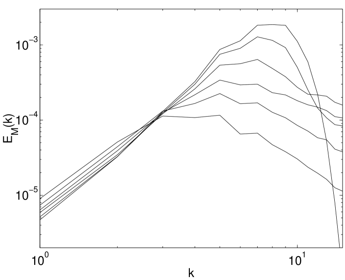
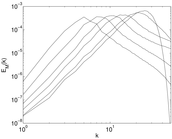
Figure 1: Magnetic energy spectrum $E_{\rm M}(k)$ for a run with unconstrained (left) and maximal (right) magnetic helicity. $\nu=\eta=5\times 10^{-5}$. The times shown are $0,1.0,4.6,10.0,21.5$ and $46.3$. At low wavenumbers $k$ the energy spectrum $E_{\rm M}(k)$ increases with time.

Turning first to maximal initial helicity, one sees that after a short initial direct cascade, there is energy transfer towards lower $k$, and the peak of the power spectrum moves to the left, signifying a growth in the coherence scale of the field. This has been called an inverse cascade, although it should be noted that the term “cascade” carries the implication of a local interaction in $k$-space, which is not necessarily true [30]. In fact, in simulations where the initial conditions contain power in only a single wavenumber, the $k^{4}$ spectrum is very quickly established at low $k$ [31], indicating that the power transfer to large scales is non-local in $k$-space [27].

For wavenumbers above the peak, one sees a decrease in power with quite a different form than is present in the initial conditions, which can be fitted approximately by $E_{\rm M}(k)\sim k^{-2.5}$.

When only helicity fluctuations are present in the initial conditions, the peak in the power spectrum still moves to low $k$, but there is very little transfer of power. It is perhaps surprising to see any transfer at all, as there are arguments which connect the evolution of the coherence length with helicity conservation [4, 20]. In an attempt to test this idea we also did a run with identical parameters but zero initial helicity, but saw essentially identical behaviour, with a small increase in power at small scales.

In our runs with $E_{\rm K}=E_{\rm M}$ initially, the kinetic energy spectrum shows no evidence of an inverse cascade at any scale. However, when the initial velocity distribution is zero the kinetic spectrum grows on all scales initially and in the low wave number region the energy continue to grow even after the high wave number modes start to decay.

6.2 Coherence length evolution

One length scale is the magnetic Taylor microscale $L_{\rm T}$, defined as $B_{\rm rms}/J_{\rm rms}$. In Fig. 2 we show $L_{\rm T}$ against time $t$ for a run with maximal initial helicity.

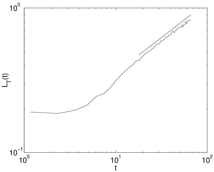
Figure 2: Time evolution of the magnetic Taylor microscale for with maximal initial magnetic helicity. $\nu=\eta=5\times 10^{-5}$. The straight line indicates the power law $\propto t^{0.5}$.

The asymptotic behaviour of the length scale is seen to grow approximately as $L_{\rm T}\sim t^{0.5}$.

In runs with non-helical initial conditions the growth of the magnetic Taylor microscale is slower: we find approximately $L_{\rm T}\sim t^{0.4}$.

6.3 Energy decay laws

Figure 3 shows the magnetic energy $E_{\rm M}(t)$ and the kinetic energy $E_{\rm K}(t)$ with maximal initial helicity.

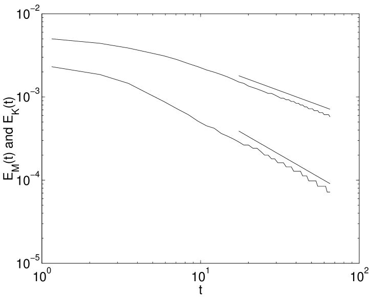
Figure 3: Time evolution of the magnetic energy $E_{\rm M}(t)$ and the kinetic energy $E_{\rm K}(t)$ in the case where there is initial magnetic helicity. $\nu=\eta=5\times 10^{-5}$. The straight lines indicate the power laws $\propto t^{-0.7}$ and $\propto t^{-1.1}$ respectively.

It is seen that the asymptotic decay rate for $E_{\rm M}(t)$ is approximately $t^{-0.7}$. The kinetic energy also decays with a power law behaviour at late times: $E_{\rm K}(t)\sim t^{-1.1}$.

In runs without initial helicity the decay rates of $E_{\rm M}(t)$ and $E_{\rm K}(t)$ are approximately the same, close to $t^{-1.1}$.

6.4 Magnetic Reynolds number

The Reynolds numbers in our simulations are evaluated using the magnetic Taylor microscale. In most our simulations we typically obtain Reynolds numbers of the order of $100-200$. In Fig. 4 we show the magnetic Reynolds number of the run with maximal helicity whose power spectrum is shown in Fig. 1.

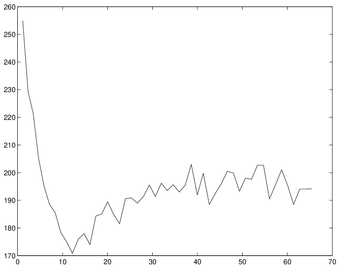
Figure 4: Magnetic Reynolds number for the run of Fig. 1

Note that for the second half of the run the magnetic Reynolds number is approximately constant.

6.5 Self-similarity in magnetic power spectrum

We make the following ansatz for the energy spectrum

$$E_{\rm M}(k,t)=\xi(t)^{-q}g_{\rm M}(k\xi),$$ (12)

where $\xi$ is the characteristic length scale of the magnetic field, taken to be the magnetic Taylor microscale defined above, and $q$ is a parameter whose value is some real number.

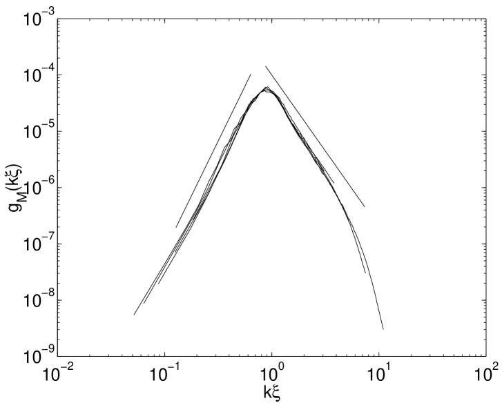
Figure 5: The magnetic scaling function $g_{\rm M}(k\xi)$ described in the text, equation (12), against $k\xi$, with power laws $(k\xi)^{4}$ and $(k\xi)^{-2.5}$ for comparison.

Figure 5 shows $\xi(t)^{q}E_{\rm M}(k,t)$ versus the scaled variable $k\xi(t)$, with $q=0.7$, plotted for different values of time $t$. The data is seen to collapse onto a single curve given $g_{\rm M}(k\xi)$: thus the magnetic field evolves in a self-similar manner.

7 Discussion and conclusions

The most directly comparable simulations of decaying 3D MHD turbulence were carried out by Biskamp and Müller [15, 16]. They found similar results, the magnetic field evolved self-similarly, with a power-law behaviour at high $k$. However, their power law was $k^{-5/3}$, much less steep than our $k^{-2.5}$. There were a number of differences between their and our simulations: they were able to achieve larger Reynolds numbers, both by having larger grids, and by using hyper-diffusivity (a $\nabla^{4}$ magnetic diffusivity term). However, we believe that the real difference is due to their initial cut-off scale being significantly larger, at $k_{c}=4$. We have performed a run with larger initial length scale, $k_{c}=5$. In this case the magnetic energy spectrum develop into an approximate $k^{-5/3}$ law at late times. However, this occurs only after the peak of the spectrum has left the simulation box.

There have also been renormalisation group (RG) analyses looking for an inverse cascade in driven MHD turbulence [21, 29]. In particular Berera and Hochberg [29] saw no evidence for an inverse cascade. However, it is not clear that the results are directly comparable, firstly because we are considering freely decaying turbulence, and secondly because RG analysis can only give information about late times when the system is in equilibrium with the driving force. What we have referred to as an inverse cascade is, even in the driven case [27], a time-dependent phenomenon characterised by a bump in the power spectrum travelling to smaller wave number.

In conclusion, we find good evidence from our numerical simulations that helical stochastic magnetic fields show an inverse cascade (in the sense explained above), and that even if only small helicity fluctuations are present initially, there is still weak inverse cascade.

We have determined growth laws for the magnetic and kinetic energies $E_{M}$ and $E_{K}$. In the helical case, $E_{M}\sim t^{-0.7}$ and $E_{K}\sim t^{-1.1}$, which means that that there is no equipartition of energy. This is because the extra constraint of helicity conservation forces the magnetic field to transfer power to larger scales rather than allow it to be dissipated. The importance of helicity is borne out by the fact that in the non-helical case, we find $\xi\sim t^{0.4}$ and $E_{M}\sim E_{K}\sim t^{-1.1}$.

Length scales in the magnetic field increase as $t^{0.5}$ in the helical case, but slightly slower in the non-helical case, $t^{0.4}$. Note that these growth laws disagree with all theoretical predictions to date [4, 18, 20, 19], which give $t^{2/3}$ in the helical case and $t^{2/7}$ for our power spectrum in the non-helical case.

Helical magnetic fields are found to evolve in a self-similar way, with a scaling function $g_{M}(z)\sim z^{-p}$ at large $k$, where $p=2.5$ for $\mathrm{Re}\sim 10^{2}$. Note that this is significantly different from both the Iroshnikov-Kraichnan and Kolmogorov spectra, $k^{-3/2}$ and $k^{-5/3}$, respectively.

A good theoretical understanding of these scaling laws is required before the evolution of magnetic fields in the early Universe is properly understood, as a small error in the exponent makes a large error in the prediction of the magnetic field strength when propagated over many orders of magnitude in time. For example, Vachaspati’s contribution to these proceedings [32] assumes a growth law of $t^{2/3}$ in the length scale, based on a simple argument invoking helicity conservation [4, 19, 20], to obtain seed fields of an interesting strength from the electroweak transition, which is quite different from our observed growth law of $t^{0.5}$.

ACKNOWLEDGEMENTS

This work was conducted on the Cray T3E and SGI Origin platforms using COSMOS Consortium facilities, funded by HEFCE, PPARC and SGI. We also acknowledge computing support from the Sussex High Performance Computing Initiative. MH thanks NORDITA for hospitality while this work was completed.

References

- [1]
- [2] Ya.B. Zeldovich, A.A. Ruzmaikin and D.D. Sokoloff, Magnetic Fields in Astrophysics (Gordon & Breach, New York, 1983); A.A. Ruzmaikin, A.A.Shukurov and D.D. Sokoloff, Magnetic Fields in Galaxies (Kluwer, Dordrecht, 1988).
- [3] P.P. Kronberg, Rep. Prog. Phys. 57, 325 (1994).
- [4] D. Biskamp, Nonlinear Magnetohydrodynamics (Cambridge Univ. Press, Cambridge, 1993).
- [5] A. C. Davis, M. Lilley and O. Tornkvist, Phys. Rev. D 60 (1999) 021301 [arXiv:astro-ph/9904022].
- [6] N.Y. Gnedin, A. Ferrara and E.G. Zweibel Astrophys.J. 539 (2000) 505-516 [arXiv:astro-ph/0001066]
- [7] M. S. Turner and L. M. Widrow, Phys. Rev. D 37 (1988) 2743.; B. Ratra, Ap. J. 391, L1 (1992); A. Dolgov, Phys. Rev. D 48 (1993) 2499 [arXiv:hep-ph/9301280].; M. Gasperini, M. Giovannini and G. Veneziano, Phys. Rev. Lett. 75 (1995) 3796 [arXiv:hep-th/9504083].; D. Lemoine and M. Lemoine, Phys. Rev. D 52 (1995) 1955.; O. Bertolami and D. F. Mota, Phys. Lett. B 455 (1999) 96 [arXiv:gr-qc/9811087]; K. Dimopoulos, T. Prokopec, O. Tornkvist and A. C. Davis, [arXiv:astro-ph/0108093].
- [8] C.J. Hogan, Phys. Rev. Lett. 51, 1488 (1983); J.M. Quashnock, A. Loeb and D.N. Spergel, Ap. J 344, L49 (1989); B. l. Cheng and A. V. Olinto, Phys. Rev. D 50 (1994) 2421; G. Sigl, A. V. Olinto and K. Jedamzik, Phys. Rev. D 55 (1997) 4582 [arXiv:astro-ph/9610201]; M. M. Forbes and A. R. Zhitnitsky, Phys. Rev. Lett. 85 (2000) 5268 [arXiv:hep-ph/0004051].
- [9] A. Vilenkin and D. Leahy, Ap. J 248, 13 (1981); Ap. J 254, 77 (1982).
- [10] M. Christensson, M. Hindmarsh and A. Brandenburg, Phys. Rev. E 64, 056405 (2001) [arXiv:astro-ph/0011321].
- [11] M. Hossain, P. Gray, D. Pontius, W. Matthaeus and S. Oughton, Phys. Fluids 7, 2886 (1995).
- [12] H. Politano, A. Pouquet and P.L. Sulem in Small-Scale Structures in Fluids and MHD, edited by M. Meneguzzi, A. Pouquet, and P.L.Sulem, Springer-Verlag Lecture Notes in Physics Vol. 462 (Springer-Verlag, Berlin, 1995), p. 281.
- [13] S. Galtier, H. Politano and A. Pouquet, Phys. Rev. Lett. 79, 2807 (1997).
- [14] M. Mac Low, R.S. Klessen, A. Burkert, and M.D. Smith, Phys. Rev. Lett.80, 2754 (1998).
- [15] D. Biskamp and W.C. Müller, Phys. Rev. Lett.83, 2195 (1999).
- [16] W.C. Müller and D. Biskamp, Phys. Rev. Lett.84, 475 (2000).
- [17] M. Hindmarsh and A. Everett, Phys. Rev. D58, 103505 (1998).
- [18] P. Olesen, Phys. Lett. B398 321 (1997) [arXiv:astro-ph/9708004].
- [19] D. T. Son, Phys. Rev. D 59 (1999) 063008 [arXiv:hep-ph/9803412].
- [20] G. B. Field and S. M. Carroll, Phys. Rev. D 62 (2000) 103008 [arXiv:astro-ph/9811206].
- [21] T. Shiromizu, Phys. Lett. B 443 (1998) 127 [arXiv:astro-ph/9810339].
- [22] A. Brandenburg, K. Enqvist, and P. Olesen, Phys. Rev. D54, 1291 (1996).
- [23] K. Subramanian and J. D. Barrow, Phys. Rev. D 58 (1998) 083502 [arXiv:astro-ph/9712083].
- [24] A. Pouquet, U. Frisch, and J. Leorat, J. Fluid. Mech. 77, 321 (1976).
- [25] M. Meneguzzi, U. Frisch, and A. Pouquet, Phys. Rev. Lett. 47, 1060 (1981).
- [26] J. Ahonen and K. Enqvist, Phys. Lett. B 382 (1996) 40 [arXiv:hep-ph/9602357]; J. Ahonen, Phys. Rev. D 59 (1999) 023004 [arXiv:hep-ph/9801434]; G. Baym and H. Heiselberg, Phys. Rev. D 56 (1997) 5254 [arXiv:astro-ph/9704214].
- [27] A. Brandenburg, ApJ 550, 824 (2001) [arXiv:astro-ph/0006186].
- [28] R. Durrer, T. Kahniashvili and A. Yates, Phys. Rev. D 58, 123004 (1998) [arXiv:astro-ph/9807089].
- [29] A. Berera and D. Hochberg, arXiv:cond-mat/0103447.
- [30] MH would like to thank Jens Niemeyer for clarification of this point.
- [31] M. Christensson, M. Hindmarsh and A. Brandenburg, in preparation.
- [32] T. Vachaspati [arXiv:astro-ph/0111124]