Faint Submillimeter Counts from Deep 850 Micron Observations of the Lensing Clusters A370, A851, and A2390

Abstract

We present deep 850 $\mu$m maps of three massive lensing clusters, A370, A851, and A2390, with well-constrained mass models. Our cluster exposure times are more than 2 to 5 times longer than any other published cluster field observations. We catalog the sources and determine the submillimeter number counts. The counts are best determined in the 0.3 to 2 mJy range where the areas are large enough to provide a significant sample. At 0.3 mJy the cumulative counts are $3.3_{1.3}^{6.3}\times 10^{4}$ deg^-2, where the upper and lower bounds are the 90% confidence range. The surface density at these faint count limits enters the realm of significant overlap with other galaxy populations.The corresponding percentage of the extragalactic background light (EBL) residing in this flux range is about $45-65$%, depending on the EBL measurement used. Given that $20-30$% of the EBL is resolved at flux densities between 2 and 10 mJy, most of the submillimeter EBL is arising in sources above 0.3 mJy. We also performed a noise analysis to obtain an independent estimate of the counts. The upper bounds on the counts determined from the noise analysis closely match the upper limits obtained from the direct counts. The differential counts from this and other surveys can reasonably be described by the parameterization $n(S)=3\times 10^{4}$ deg^-2 mJy${}^{-1}/(0.7+S^{3.0})$ with $S$ in mJy, which also integrates to match the EBL.

1. Introduction

The cumulative emission from all sources lying beyond the Galaxy, the extragalactic background light (EBL), provides important constraints on the integrated star formation and accretion histories of the Universe. COBE measurements of the EBL at far-infrared (FIR) and submillimeter wavelengths (e.g., Puget et al. 1996; Fixsen et al. 1998) indicate that the total radiated emission that is absorbed by dust and gas and then reradiated into the FIR/submillimeter is comparable to the total measured optical EBL. Deep submillimeter surveys with SCUBA (Holland et al. 1999) on the James Clerk Maxwell Telescope have uncovered the brighter obscured sources which give rise to a substantial part of the FIR/submillimeter EBL. The properties of these sources are similar to the properties of the most luminous systems observed locally, the ultraluminous infrared galaxies (ULIGs, Sanders & Mirabel 1996).

Blank field SCUBA surveys have resolved sources over the $2-10$ mJy range that account for $20-30$% of the 850 $\mu$m EBL (e.g., Barger et al. 1998; Hughes et al. 1998; Eales et al. 1999, 2001; Barger, Cowie, & Sanders 1999a; Scott et al. 2002; Borys et al. 2002; Webb et al. 2002). Barger et al. (1999a) found that their cumulative source counts per square degree were well described by the power-law parameterization of the differential counts

$$n(S)=N_{0}/(a+S^{\alpha})$$

with $S$ in mJy, $\alpha=3.2$, and $N_{0}=3.0\times 10^{4}$ deg^-2 mJy^-1. Assuming only that their parameterization provided an appropriately smooth continuation to fluxes below 2 mJy, Barger et al. (1999a) constrained their fit to match the EBL with $a\sim 0.5$. Using this empirical parameterization, they predicted that very approximately 60% of the EBL at 850 $\mu$m should be resolved into discrete sources between 0.5 and 2.0 mJy.

Blank field SCUBA surveys cannot reach the required sensitivities to directly detect the dominant population of $<2$ mJy extragalactic sources due to confusion noise resulting from the coarse resolution of SCUBA (e.g., Hogg 2001). Thus, in order to search for this population with SCUBA, one must observe fields with massive cluster lenses to take advantage of both gravitational amplification by the lens and reduced confusion noise. Smail, Ivison, & Blain (1997) and Smail et al. (1998) pioneered this method, making the first SCUBA observations of cluster lenses. They studied seven clusters with well-constrained lens models where it is possible to correct the observed source fluxes for lens amplification. Their survey was designed to detect the brightest submillimeter sources in relatively short integration times, and hence it is quite shallow with $3\sigma$ flux limits around 6 mJy.

Despite the shallowness of the survey, Blain et al. (1999) tried to determine the number counts at and below 1 mJy, arguing that the small regions of high amplification (around a factor of 6 at 1 mJy and a factor of 24 at 0.25 mJy) could be used to probe these faint fluxes. (A later analysis of another cluster sample of similar depth by Chapman et al. (2002) did not extend the counts below 1 mJy.) However, direct inversion at these amplification levels is complicated because redshift uncertainties and small positional changes can have large effects on the amplification. In SCUBA surveys the positions of the submillimeter sources are relatively poorly determined and the redshifts are often unknown. While these effects have comparatively little effect on the shape of the determined counts, they do effectively limit the flux level to which the counts can be considered to be determined. We shall discuss this point further in § 4.

The sub-mJy counts are best addressed by obtaining much deeper images, since at lower amplifications there is considerably less redshift and positional sensitivity. At typical amplifications of 1 to 4, the counts can be robustly investigated down to a few tenths of a mJy from images with $3\sigma$ limits of 1.5 to 2 mJy. Because of this key point, and because the observed areas at the sub-mJy fluxes of interest rise rapidly with deeper obervations, it is a natural and important progression to pursue the faint submillimeter counts with much longer integrations on lensing cluster fields. This is the subject of the present paper.

2. Observations and Sample

SCUBA jiggle map observations were taken in mostly excellent observing conditions during runs in 1999 August, September, and November; 2000 November and December; and 2001 January, March, and June. The maps were dithered to prevent any regions of the sky from repeatedly falling on bad bolometers. The chop throw was fixed at a position angle of 90 deg so that the negative beams would appear $45^{\prime\prime}$ on either side east-west of the positive beam. Regular “skydips” (Lightfoot et al. 1998) were obtained to measure the zenith atmospheric opacities at 450 and 850 $\mu$m, and the 225 GHz sky opacity was monitored at all times to check for sky stability. Pointing checks were performed every hour during the observations on the blazars 0106+013, 0215+015, 0221+067, 0336-019, 0420-014, 0917+449, 0923+392, 2145+067, or 2251+158.

The data were reduced using the dedicated SCUBA User Reduction Facility (SURF, Jenness & Lightfoot 1998). Due to the variation in the density of bolometer samples across the maps, there is a rapid increase in the noise levels at the very edges, so the low exposure edges were clipped. The data were calibrated using jiggle maps of the primary calibration source Mars or the secondary calibration sources CRL618, CRL2688, or OH231.8+4.2. The routines produce a noise-weighted exposure time at each pixel, which we shall denote as $t$. Submillimeter fluxes were measured using beam-weighted routines that include both the positive and negative portions of the beam profile to provide the optimal extraction.

The SURF reduction routines arbitrarily normalize all the data maps in a reduction sequence to the central pixel of the first map; thus, the noise levels in a combined image are determined relative to the quality of the central pixel in the first map. In order to determine the absolute noise levels of our maps, we first eliminated the $\gtrsim 3\sigma$ real sources in each field by subtracting an appropriately normalized version of the beam profile. We then iteratively adjusted the noise normalization until the dispersion of the signal-to-noise ratio measured at random positions became $\sim 1$. This noise estimate includes both fainter sources and correlated noise; hereafter we refer to it as “uncleaned noise”.

We also constructed “true noise” maps in which all the sources have been cleaned out so that the maps contain only sky and bolometer noise. To do this, we divided the data for each cluster into two halves and then combined the jiggle maps for each of the two halves separately, keeping only the first jiggle map in the reduction sequence the same in both halves, since the data maps are normalized to the central pixel of the first map. We then subtracted the two halves from one another. Since the faint sources are at fixed positions in the maps, the subtraction effectively removes them from the maps, resulting in true noise maps for each cluster field. The true noise maps were then scaled to the actual maps by multiplying each pixel by the factor $(t_{1}+t_{2})/\sqrt{(t_{1}\times t_{2}})$, where $t_{1}$ and $t_{2}$ are the weighted exposure times in the two half images.

The three cluster field centers, total SCUBA exposure times (based on the number of integrations), median optical depths, areas, and 850 $\mu$m sensitivities ($1\sigma$) for the true noise maps and the uncleaned noise maps are given in Table 1. Our cluster exposure times are more than 2 to 5 times longer than any other published cluster field observations (Smail et al. 1997, 1998; Chapman et al. 2002). Our three cluster field SCUBA maps and their corresponding true noise maps are shown in Fig. 1.

3. Source Catalogs and Identifications

In contrast to the situation in the optical and near infrared, we do not expect there to be much contamination of the background submillimeter number counts by cluster members, which lie at too low redshifts to be strong submillimeter sources. However, there may be submillimeter sources produced by the cooling flow regions in the clusters and the associated strong radio sources in some of the central cluster galaxies (Edge et al. 1999). In particular, Edge et al. report a strong source associated with the cD galaxy in A2390. We therefore searched the images for sources of this type. Table 2 gives the source number, measured positions (columns 2 and 3), measured submillimeter fluxes and uncertainties (column 4), and measured signal-to-noise ratios (column 5) for the D cluster galaxies in A370 and A851 and the cD galaxy in A2390. We confirm the detection of the cD galaxy in A2390 and also find a source associated with the southern D galaxy in A370. These two sources were removed from the maps by subtracting a normalized image of the beam.

To generate the catalog of the background submillimeter galaxies, we next scanned the three SCUBA maps at an array of positions separated by $3^{\prime\prime}$ to make a preliminary selection of candidate sources. Using peaked-up positions, we then located the $\geq 3\sigma$ sources. We subtracted the brighter sources from the maps before extracting the fainter sources in order to avoid contamination by the large and complex beam pattern. Table 3 summarizes the information for the background sources in the same format as Table 2. Only sources with weighted exposure times greater than a tenth of the maximum in the image are included, giving a total sample of 15 sources. For the purpose of the counts analysis, the $3\sigma$ selection is reasonable; however, considerable caution should be used in interpreting sources at this low significance level since there may be substantial uncertainties in both position and flux. Our simulations (see § 4) suggest that interpretation of individual sources and attempts to identify counterparts are best restricted to at least the $\geq 4\sigma$ subsample (see also Scott et al. 2002). In the last three columns of Table 3 we give the previous submillimeter flux measurements from Smail et al. (1997, 1998) for the sources detected in their shallow survey, along with the RA and Dec offsets between our measured source positions and theirs. In general the fluxes agree to within the noise uncertainty. However, the offsets in position range up to $4^{\prime\prime}$ for the faintest overlapping source.

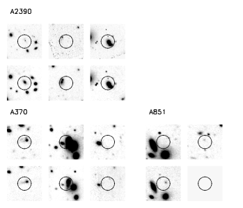
Figure 2.— $K$ (lower panel) and $I$ (upper panel) thumbnail images for the $4\sigma$ sources in Table 1. The ordering within each cluster (left = submillimeter bright to right = submillimeter faint) follows that of Table 3. The panels are $19^{\prime\prime}$ on a side, centered on the nominal SCUBA position. The circles are of radius $3.5^{\prime\prime}$, which is representative of the positional uncertainty. North is up and East is to the right.

Efforts to spectroscopically identify the counterparts to the SCUBA sources have proved difficult due to the optically faint nature of the majority of the counterparts; however, high-quality optical images, extremely deep radio maps, and follow-up optical spectroscopy suggest that the bulk of the submillimeter sources lie in the redshift range $z=1-3$ (e.g., Smail et al. 1998; Barger et al. 1999b; Smail et al. 2000; Carilli & Yun 2000; Barger, Cowie, & Richards 2000; see, however, Lilly et al. 1999).

In Fig. 2 we show $I$ and $K$-band thumbnail images of the eight $4\sigma$ sources in the sample, according to cluster. The image is taken from E.M. Hedrick, A.J. Barger, & J.-P. Kneib, in preparation, where the data reduction and photometry of the sources are described. The two brightest submillimeter sources in A370 both have spectroscopic redshifts ($z=2.80$ from Ivison et al. 1998 and $z=1.06$ from Barger et al. 1999b and Soucail et al. 1999), which we give in column 7 of Table 2. The other two sources with previous discussions in the literature are the brightest submillimeter source in A851, believed to be associated with the extremely red object (ERO) in the error circle (Ivison et al. 2000), and the second brightest submillimeter source in the A2390 sample. The most likely counterpart to the latter is thought to be the ERO at $z=1.02$, which is to the West of the thumbnail center in Fig. 2. This source (designated K3 in Barger et al. 1999b where the redshift was given) is also a weak ISOCAM source (Lemonon et al. 1999). However, the large separation from the Smail et al. position ($6.3^{\prime\prime}$) made the identification suspect. With the new position the source now lies within the submillimeter error circle, and we now consider this identification to be highly probable. We give this redshift in Table 2.

The remaining sources are most likely associated with EROs in their error circles. In particular, the brightest A2390 submillimeter source is associated with a very luminous ERO, which is also a weak ISOCAM source (Lemonon et al. 1999). We do not know of a spectroscopic identification for this source. The weakest of the three $4\sigma$ A2390 sources lies near a bright spectroscopically confirmed cluster member. It appears unlikely this is the correct identification of the source, which may be associated with one of the fainter galaxies in this area. The effects of excluding this source from our subsequent analysis are small. A more extensive discussion of the submillimeter properties of the optical and near-infrared selected galaxies in these fields may be found in E.M. Hedrick, A.J. Barger, & J.-P. Kneib, in preparation.

The observed sources directly determine the fraction of the EBL which has been resolved, since the average sky brightness is conserved by the lensing process. This is by far the most robust quantity which can be derived from the observations (Chapman et al. 2002). The average EBL contribution of the three fields is 17.3 Jy deg^-2, and the breakdown by field is 22.7 Jy deg^-2 (A370), 17.4 Jy deg^-2 (A851), and 11.8 Jy deg^-2 (A2390), with the differences reflecting the different depths of the images and the statistical uncertainties from the small numbers of sources involved. The average over the three fields is between 40% and 56% of the total EBL, depending on whether we adopt the EBL value of 44 Jy deg^-2 (Fixsen et al. 1998) or 31 Jy deg^-2 (Puget et al. 1996). However, detailed models are required to determine the flux ranges which give rise to this contribution. The contribution to the EBL from sources greater than 6 mJy (roughly previous survey limits) is 7.8 Jy deg^-2; thus, the increased sensitivity roughly doubles the resolved fraction of the EBL in these clusters.

4. Direct Number Counts

For a blank field observation, the number counts are determined by dividing the number of significantly detected sources in a sample by the area over which the sources could be detected at that level. In the case of a lensed field, the sensitivity to a background source is dependent on the position and redshift of the background source and on the redshift of the gravitational lens. These lensing effects can be corrected for with a sufficiently detailed mass model for the lens.

We used the LENSTOOL models to determine the flux amplifications. LENSTOOL uses multiple-component mass distributions that describe the extended potential well of the clusters and their more massive individual member galaxies (e.g., Kneib et al. 1996). The mass distributions are derived from the positions of multiply-imaged features identified in high-resolution optical images; spectroscopic redshifts constrain the models. Details of the models for the A370, A851, and A2390 clusters can be found in Kneib et al. (1993), Seitz et al. (1996), and Kneib et al., in preparation, respectively. Using LENSTOOL we mapped the background galaxies from their observed positions back onto the source plane using known redshifts, where available, or to an assumed source redshift of $z=3$. We give the resulting amplifications in column 6 of Table 3.

Although the amplification of a source depends on both the redshift of the lens and the redshift of the source, at the redshifts of our three cluster lenses ($z=0.37$ for A370, $z=0.41$ for A851, and $z=0.23$ for A2390), the amplification varies only weakly with redshift for any source beyond $z=1$ which has a modest amplification. Blain et al. (1999) estimated that as long as the source redshifts are greater than one, the systematic uncertainties (due to the uncertainties in both the redshift distribution of the detected sources and the mass models of the clusters) are less than 25% and hence are comparable to the typical uncertainties in the absolute flux calibration of the SCUBA maps.

However, sources with high amplifications have much larger uncertainties associated with positional uncertainty and redshift indeterminancy than sources with relatively low amplifications. For the high amplification sources lying near critical lines, small changes in position or redshift can result in very large variations in amplification. In order to quantify this effect, we computed the maximum and minimum amplifications in a $3^{\prime\prime}$ radius region surrounding each source. For the sources where we do not have a refined position from an optical identification, we give this range in brackets after the amplification in Table 3. For sources with “typical” amplifications of 1 to 4 the effect is generally small. However, the high amplification sources can easily have order of magnitude amplification uncertainties associated with their positions (and also with their redshifts), and this must be allowed for in any analysis.

Five of the sources in our sample (two in A370 and three in A2390) fall into this category. All lie at the faint end of the sample where we cannot easily use secondary constraints, such as the lack of multiple images, to provide limits on the amplifications. For two of the sources in A2390 (13 and 14 in Table 3) there are no sensible upper limits to the amplifications, so we give only lower bounds. In what follows we use the maximum and minimum amplifications given in Table 3 to determine how much the number counts can be changed by the amplification uncertainties.

For the direct number counts, we need to know the source plane areas for which background galaxies would fall within the SCUBA maps and be significantly detected. (Due to the expansion of the source plane, the source plane areas are smaller than the areas of the SCUBA maps.) To do this, we created a grid of $z=3$ background sources at one arcsecond separations and used LENSTOOL to produce the corresponding image plane maps with magnifications $m$. (For sources with known redshifts, we created the source plane grids at the known redshifts.) Each grid point on the image plane corresponds to an area on the source plane of 1 arcsec². If the sensitivities of the SCUBA maps were uniform, we could determine the source plane area for a $3\sigma$ detection at a given submillimeter flux by finding the number of points at each image plane grid point that satisfied the equation $3\sigma/mf(850~{}\mu$m) and then multiplying that number by 1 arcsec².

However, since the SCUBA maps become less sensitive towards the edges where the exposure times are less, the equation to be satisfied is instead $3\sigma_{min}/(m\sqrt{t/t_{max}})<f(850~{}\mu$m), where $\sigma_{min}$ is the minimum noise in the field and $t_{max}$ is the maximum weighted exposure time. The number of points satisfying this equation can then be multiplied by 1 arcsec².

Figure 3.— Source plane areas, assuming source redshifts $z=3$, over which a source of a given flux in the source plane would be detected at the $3\sigma$ level in the image plane. The three curves are for the A370 (solid), A851 (dotted), and A2390 (dashed) fields. The horizontal line segment shows the SCUBA map area.

Figure 4 shows the areas over which a source with a given flux in the source plane would be detected at the $3\sigma$ level in the image plane for each of the three cluster fields. The high magnification of the A370 cluster lens means there is less source plane area at high submillimeter fluxes in the A370 field but much more source plane area at low submillimeter fluxes. The SCUBA data available on A370 are deeper than the data on the other two clusters, which also contributes to the sizeable differences in source plane areas seen in Fig. 4 at the fainter fluxes.

Figure 4.— Cumulative 850 $\mu$m source counts (solid squares). The solid curve shows an area-weighted maximum likelihood power-law fit to the data (solid squares) over the flux range from 0.1 mJy to 5 mJy. The slope is $-1.1$. The open triangles show the counts determined if we use the minimum amplifications of Table 3. The open diamonds show the counts determined if we use the maximum amplifications.

We can now determine our raw cumulative source counts by summing the inverse areas of all the sources in the three fields brighter than flux $S$. We present these raw cumulative 850 $\mu$m counts per square degree (solid squares) in Fig. 4. We also show as the open symbols the counts computed using the minimum (triangles) and maximum (diamonds) amplifications of Table 3. The shape and the normalization of the counts are quite insensitive to the choice of minimum or maximum amplifications (see also Chapman et al. 2002). However, the flux to which the counts can be considered to be determined does depend critically on the amplification.

In the present data, if we adopt the minimum amplifications, then the counts only extend down to 0.1 mJy. However, if we were instead to assume that the average or maximum amplifications were appropriate, then the counts would extend to much fainter fluxes ($<0.1$ mJy). Because the areas of high amplification are small, this would then imply that the counts turn up quite steeply below 0.1 mJy in order for us to actually be able to detect sources in such small areas. Indeed, in the maximum amplification case, two of the sources even lie below the 0.01 mJy flux limit of Fig. 4. However, since we have a perfectly adequate solution with the minimum amplifications, at present we have no way of knowing whether there really are sources at fluxes below 0.1 mJy. To avoid this uncertainty, for the remaining discussion of the counts we shall restrict ourselves to fluxes above 0.1 mJy.

We have overplotted on the figure a power-law fit (solid line) to the solid squares based on an area-weighted maximum likelihood fit (Crawford, Jauncey, & Murdoch 1970), which gives a slope of $-1.1$ and provides a good representation of the raw counts. Given the complex effects of noise and confusion, the errors and systematic biases of the counts are best estimated with Monte Carlo simulations.

5. Simulations

We created simulated images by drawing sources from a population with a count described by the power-law fit and placing them randomly on the source plane. We limited the fluxes of the input sources to be brighter than 0.01 mJy. We then mapped and amplified the sources to the image plane using LENSTOOL and added the sources into the true noise maps. We analyzed the resulting images with the same procedures that we used to analyze the real data. We ran 100 realizations for each field and derived the average output counts. We then iteratively adjusted the input count model until the average output counts matched the observed counts. For the final determination of the counts completeness and confidence ranges we used the input power-law

$$N(>S)=3.5\times 10^{3}\times(S/2~{}{\rm mJy})^{-1.2}~{}{\rm deg}^{-2}$$ (1)

shown by the dashed line in Fig. 5. The solid line in Fig. 5 shows the recovered counts obtained for this input count model. The recovered counts can be compared with the observed raw counts, which are shown by the solid squares in Fig. 5. The recovered counts exhibit a small systematic upward (Eddington) bias relative to the input counts at the brighter fluxes. Over the 1 to 5 mJy range we see an increase by a factor of 1.25. Eales et al. (2000) and Scott et al. (2002) obtained a similar systematic flux boost from their simulations. Eales et al. found a median boost factor of 1.44 for their survey down to 3 mJy, and Scott et al. found boost factors of 1.28 and 1.35 at 5 mJy for their two areas. The shallower slope of the counts in the present simulation may account for the slightly smaller correction. At low fluxes the recovered counts drop below the input counts as the source detection becomes incomplete.

The uncertainty corridors for the counts may also be obtained by looking at the spread of counts over the various realizations. The 90% confidence range measured in this way from the simulations is shown by the thin solid lines and should provide a good estimate of the uncertainties on the observed counts.

Figure 5.— Comparison of the observed counts (solid boxes) with the simulations. The solid curve shows the returned counts from the Monte Carlo simulations, which were based on an input model described by a power-law fit (dashed line). Eddington bias raises the measured counts above the input counts at the high flux end, while at the low end incompleteness in the source detection drops the measured counts below the input counts. The thin solid lines show the 90% confidence range calculated using the simulations.

As is evident from Fig. 5, the counts are best determined in the 0.3 to 5 mJy flux range. Here the areas are large enough to provide a significant sample. However, the statistical uncertainties are still large with only 7 sources lying in this range. At 1 mJy we find a cumulative count of $0.9_{0.5}^{1.4}\times 10^{4}$ deg^-2, after correcting for the systematic upward bias, where the upper and lower bounds are the 90% confidence range. This is consistent with the Blain et al. (1999) measurement of $(0.79\pm 0.3)\times 10^{4}$ deg^-2. At 0.3 mJy the cumulative counts have risen to $3.3_{1.3}^{6.3}\times 10^{4}$ deg^-2, where the upper and lower bounds are again the 90% confidence range.

6. Noise Analysis

The noise distributions of the uncleaned noise maps (i.e., the maps with the directly detected sources removed) contain additional independent information over the direct counts. In principle, the noise distributions should provide a more sensitive diagnostic of the counts at sub-mJy fluxes than the direct counts because the useable areas are much larger than the areas over which $3\sigma$ sources can be detected.

In Fig. 6 we show the distribution functions (combined for all three cluster fields) from both the true noise and the uncleaned noise maps. The true noise distribution function is well fit by a smooth Gaussian function, which is shown in the figure in place of the actual distribution function. The uncleaned noise distribution function (jagged curve) has extensions to the right and left of the true noise distribution function. The different shapes of these two extensions result from there being twice as many negative positions as positive positions in the beam pattern corresponding to each source, but at half the flux (because of the nod and fixed chop observing procedure used). For the present data a Kolmogorov-Smirnov test (applied to the absolute values of the distribution to combine the two tails of the distribution function) does not reject the hypothesis that the uncleaned noise distribution is drawn from the true noise distribution because there are a relatively small number (approximately 240) of independent points in the fields. A noise analysis is therefore primarily useful in placing an upper bound on the counts.

Figure 6.— Distribution function for the three fields. The true noise is well fit by a smooth Gaussian function (solid curve). The extensions of the uncleaned noise (jagged curve) indicate the presence of faint sources below the detection limit. The differences between the right-hand and left-hand extensions result from there being twice as many negative positions as positive in the beam pattern corresponding to a given source, but at half the flux.

The difference between the observed uncleaned and the simulated uncleaned distribution functions can be used to constrain the simulated counts distribution. If the input function for the counts has too high a normalization or is too steep at the faint end, then the simulated distribution will be too wide when compared to the observed distribution. In contrast, if the input function has too low a normalization or is too shallow at the faint end, then the simulated distribution will be too narrow when compared to the observed distribution.

We performed Monte Carlo simulations using two different parameterizations to determine the number counts at faint fluxes. In the first case we used the Barger et al. (1999a) parameterization

$$n(S)=N_{o}/(a+S^{\alpha})$$ (2)

with $S$ in mJy, which fit their differential blank field counts above 2 mJy for $\alpha=3.2$ and $N_{o}=3.0\times 10^{4}$ deg^-2 mJy^-1. Here we varied $a$. In the second case we used a power-law parameterization of the faint counts normalized to match the Barger et al. counts and the present direct counts at 2 mJy. Here we varied the power-law index.

Sources were drawn from a population with a count described by the chosen model. For each of the two models we performed 100 realizations at each value of the index. For each realization we randomly populated the source plane of each cluster, assuming source redshifts of $z=3$. The source plane sources were then mapped onto the image plane using the LENSTOOL model and added into the true noise map of the field to construct the simulated image.

Figure 7.— The dashed curve shows the 90% confidence upper limits from Monte Carlo simulations that assumed the parameterization of Barger et al. (1999a), $n(S)=N_{o}/(a+S^{\alpha})$, with $N_{o}=3.0\times 10^{4}$ deg^-2 mJy^-1 and $\alpha=3.2$; the value of $a$ for the curve is 0.13. The solid power-law curve shows the 90% confidence limit from Monte Carlo simulations that assumed a power-law parameterization. The power-law index is 2.1. The solid boxes show the direct counts and the jagged curves show the 90% confidence range on the direct counts.

We measured the simulated distribution functions in the same way that we measured the uncleaned noise distribution function. That is, we first removed all $>3\sigma$ sources in order to sample the effect of the faint sources. We then applied a Kolmogorov-Smirnov test to compare the simulated distributions with the observed uncleaned distribution. We found that at the 90% confidence level the index $a$ in the Barger et al. (1999a) parameterization cannot be less than 0.13, and the power-law index cannot exceed 2.1. These upper bounds are shown as the dashed line and solid power-law, respectively, in Fig. 6. These independent estimates from the noise analysis closely match the upper limits from the direct counts over the flux range above 0.2 mJy but place a somewhat tighter constraint at 0.1 mJy where the 90% confidence limit on the cumulative counts is $1.5\times 10^{5}~{}{\rm deg}^{-2}$ for the power-law model.

7. Discussion

We summarize the current results and compare them with wide-field blank surveys in Fig. 7. The present data are shown by the solid squares. We show the lensing analysis of Blain et al. (1999) as open circles and that of Chapman et al. (2002) as open downward pointing triangles. The present analysis shows good overlap with that of Blain et al. at the brighter fluxes, though both are slightly lower than that of Chapman et al. In order to show the counts at bright fluxes we have plotted the blank field surveys of Barger, Cowie, & Sanders (1999), Hughes et al. (1998), Eales et al. (2000), Scott et al. (2002), and Borys et al. (2002). The large area survey of Scott et al. and the Hubble Deep Field scan map point of Borys et al. produce slightly shallower counts than the other surveys.

We show a simple broken power-law fit to the counts in Fig. 7 where the differential counts are given by

$$n(S)=N_{0}/S^{\alpha}$$ (3)

with $N_{0}=2.5\times 10^{4}$ deg^-2 mJy^-1 and $\alpha=3.0$ above $S=3$ mJy and $N_{0}=1\times 10^{4}$ deg^-2 mJy^-1 and $\alpha=2.2$ below 3 mJy. The EBL in this representation diverges at the faint end. We plot the Barger et al. (1999) parametric fit for two values of $\alpha$ (dashed line shows 3.0, dotted line shows 3.2), $N_{0}=3\times 10^{4}$ deg^-2 mJy^-1, and $a=0.7$ and $a=0.5$, respectively. Both curves give an integrated surface brightness set to match the EBL measurement of Fixsen et al. (1998) and provide reasonable descriptions of the counts, though the shallower model may be preferred as a better match to the Scott et al. (2002) data.

Figure 8.— A summary of the counts and 90% confidence limits between 0.2 and 3 mJy from the analysis of § 5 is shown by the solid squares and associated uncertainties. The upper limit at 0.1 mJy, based on the noise analysis of § 6, is shown as a downward pointing arrow. The open circles show the points from Blain et al. (1999). These have been slightly displaced to larger fluxes to distinguish them from the present counts. The Blain et al. point at 0.5 mJy is shown as a $2\sigma$ upper limit for consistency with the present analysis. The open downward pointing triangles show the cluster lensing analysis counts of Chapman et al. (2002). All of the lensing analysis data is only shown below a flux of 5 mJy. We include the wide-field counts of Barger, Cowie, & Sanders (1999) (open diamonds), Hughes et al. (1998) (crosses), Eales et al. (2000) (open squares), Scott et al. (2002) (open triangles), and Borys et al. (2002) (asterisk), but we only show $1\sigma$ uncertainties for the Scott et al. data to avoid confusing the plot; the uncertainties on the other surveys are larger. We show the Barger, Cowie, & Sanders (1999) parametric fit (dotted line) and an alternate version (dashed line) of this parametric fit discussed in the text, which provides a better match to the Scott et al. data; it also integrates to match the EBL. We also show a broken power-law representation of the data with slope $-2$ above 3 mJy and $-1.2$ below 3 mJy. This representation is divergent at faint fluxes and must turn over further at some point.

The contribution to the EBL in the 0.3 to 2 mJy flux range can be directly measured from our counts and is $2.0_{0.8}^{3.2}\times 10^{4}$ mJy deg^-2, where the upper and lower bounds are the 90% confidence range. Thus, the percentage of the EBL residing in this range is $65_{26}^{100}$%, if we adopt the 850 $\mu$m EBL measurement of $3.1\times 10^{4}$ mJy deg^-2 from Puget et al. (1996), or $45_{18}^{72}$%, if we adopt the measurement of $4.4\times 10^{4}$ mJy deg^-2 from Fixsen et al. (1998). Given that $20-30$% of the EBL is resolved at fluxes between 2 and 10 mJy (Barger et al. 1999a; Eales et al. 1999, 2001, Scott et al. 2002), it appears that most of the submillimeter EBL is arising in sources brighter than 0.3 mJy.

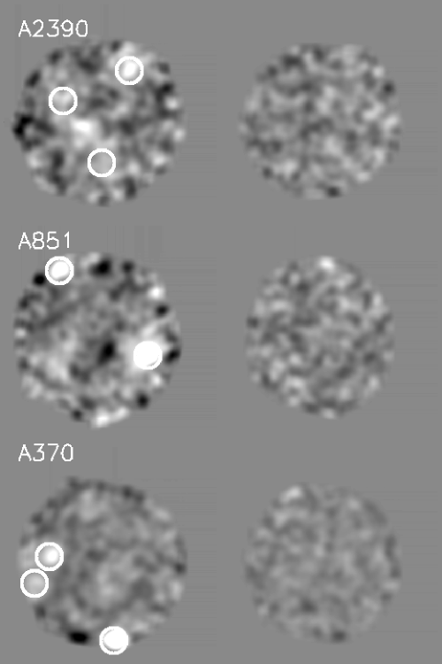
Figure 1.— SCUBA maps of the A370, A851, and A2390 cluster fields (left) and their corresponding true noise maps (right). The $4\sigma$ sources listed in Table 3 are circled in the cluster images in the left-hand panels.

Table 1SCUBA Observations of the A370, A851, and A2390 Fields

Cluster	RA(2000)	Dec(2000)	Total Exposure	Median	Area	True Noise	Uncleaned Noise
			Time (ks)	$\tau(850~{}\mu$m)	(arcmin2)	($1\sigma$)(mJy)	($1\sigma$)(mJy)
A370	2 39 53.10	$-1$ 34 35.0	133.1	0.18	6.3	0.35	0.45
A851	9 42 59.65	46 58 57.0	59.3	0.27	6.3	0.80	0.87
A2390	21 53 35.55	17 41 52.3	78.1	0.26	6.3	0.69	0.71

Table 2Cluster Submillimeter Sources in the A370, A851, and A2390 SCUBA Fields

#	RA(2000)	Dec(2000)	$f(850~{}\mu$m)	S/N
			(mJy)
C0	2 39 53.07	$-1$ 34 55.7	$1.97\pm 0.46$	4.34
C1	2 39 52.69	$-1$ 34 18.6	$-0.41\pm 0.46$	$-0.90$
C2	9 42 56.14	46 59 12.5	$0.36\pm 1.05$	0.35
C3	9 42 57.93	46 59 12.7	$-1.93\pm 0.95$	$-2.04$
C4	21 53 36.75	17 41 44.2	$6.96\pm 0.67$	10.39

Table 3Background Submillimeter Sources in the A370, A851, and A2390 SCUBA Fields

#	RA(2000)	Dec(2000)	$f(850~{}\mu$m)	S/N	Amplification	$z$	Smail et al.	RA Offset	Dec Offset
		(mJy)			(min, max)		$f(850~{}\mu$m)(mJy)	(sec)	(arcsec)
0	2 39 51.90	$-1$ 35 59.0	$21.06\pm 1.34$	15.73	2.3	2.80	23.0	$-0.00$	0.0
1	2 39 56.63	$-1$ 34 27.0	$6.68\pm 0.58$	11.58	2.3	1.06	11.0	$-0.23$	0.0
2	2 39 57.64	$-1$ 34 56.0	$3.49\pm 0.66$	5.29	1.9 (1.8,2.0)	$\cdots$	$\cdots$	$\cdots$	$\cdots$
3	2 39 58.57	$-1$ 34 34.0	$2.52\pm 0.74$	3.40	1.7 (1.6,1.7)	$\cdots$	$\cdots$	$\cdots$	$\cdots$
4	2 39 53.83	$-1$ 33 37.0	$2.17\pm 0.57$	3.82	7.3 (5.6,10.8)	$\cdots$	$\cdots$	$\cdots$	$\cdots$
5	2 39 52.63	$-1$ 34 40.0	$1.39\pm 0.45$	3.09	10 (4.2,43)	$\cdots$	$\cdots$	$\cdots$	$\cdots$
6	2 39 47.36	$-1$ 35 07.0	$2.49\pm 0.72$	3.43	1.6 (1.6,1.7)	$\cdots$	$\cdots$	$\cdots$	$\cdots$
7	9 42 54.57	46 58 44.0	$15.06\pm 1.07$	14.02	1.5 (1.5,1.6)	$\cdots$	17.2	0.13	0.0
8	9 43 03.96	47 00 16.0	$10.46\pm 1.83$	5.72	1.2 (1.2,1.2)	$\cdots$	$\cdots$	$\cdots$	$\cdots$
9	9 42 53.49	46 59 52.0	$4.93\pm 1.49$	3.30	1.3 (1.3,1.4)	$\cdots$	$\cdots$	$\cdots$	$\cdots$
10	21 53 33.31	17 42 49.3	$7.57\pm 0.93$	8.14	1.9 (1.8,2.0)	$\cdots$	$\cdots$	$\cdots$	$\cdots$
11	21 53 38.35	17 42 16.3	$4.52\pm 1.04$	4.35	1.9	1.02	6.7	0.15	3.3
12	21 53 35.48	17 41 09.3	$3.24\pm 0.78$	4.15	52 (0.6,52)	$\cdots$	$\cdots$	$\cdots$	$\cdots$
13	21 53 38.21	17 41 52.3	$2.64\pm 0.72$	3.64	11 ($>6.7$)	$\cdots$	$\cdots$	$\cdots$	$\cdots$
14	21 53 34.15	17 42 02.3	$2.64\pm 0.72$	3.42	39 ($>15$)	$\cdots$	$\cdots$	$\cdots$	$\cdots$