GALAXIES ASSOCIATED WITH $z\sim 4$ DAMPED Ly$\alpha$ SYSTEMS I. IMAGING AND PHOTOMETRIC SELECTION

Abstract

This paper describes the acquisition and analysis of imaging data for the identification of galaxies associated with $z\sim 4$ damped Ly$\alpha$ systems. We present deep $BRI$ images of three fields known to contain four $z\sim 4$ damped systems. We discuss the reduction and calibration of the data, detail the color criteria used to identify $z\sim 4$ galaxies, and present a photometric redshift analysis to complement the color selection. We have found no galaxy candidates closer to the QSO than $7^{\prime\prime}$ which could be responsible for the damped Ly$\alpha$ systems. Assuming that at least one of the galaxies is not directly beneath the QSO, we set an upper limit on this damped Ly$\alpha$ system of $L<L_{LBG}^{*}/4$. Finally, we have established a web site to release these imaging data to the public (http://kingpin.ucsd.edu/$\sim$dlaimg).

Accepted to the Astronomical Journal: Jan 22, 2002

1 INTRODUCTION

In this era of large telescopes, it is almost routine to identify galaxies at high redshift. Deep narrow band imaging (e.g. Hu et al., 1998) and the Lyman break technique (Steidel & Hamilton, 1993), among other approaches, have led to the discovery of over 1000 $z>2$ galaxies where just 10 years ago only a handful were known. Unfortunately, because these techniques are magnitude limited, they are primarily sensitive to the high luminosity tail of the protogalactic distribution. For example, the Lyman break galaxies exhibit a two-point correlation function which suggests they are massive galaxies associated with significant large-scale structures (Adelberger et al., 1998) that will evolve into the most massive galaxies today. To study the formation of typical galaxies, therefore, one must circumvent this luminosity selection.

Even before the recent outburst of high redshift galaxy identifications, researchers had already discovered a significant population of high $z$ protogalaxies in absorption: the damped Ly$\alpha$ systems (e.g. Wolfe et al., 1986). Because the selection of these galaxies is based on H I gas cross-section, they are predicted to sample the bulk of the galactic mass distribution (Kauffmann, 1996) and therefore provide a broader picture of galaxy formation in the early universe. Attempts to identify in emission the galaxies which give rise to damped systems, however, have met with limited success. Djorgovski and collaborators (Djorgovski et al., 1996; Djorgovski, 1997) have made a few discoveries, but their success rate is uncertain. More recently, Warren et al. (2001) have analysed deep HST images of fields around quasars known to exhibit damped Ly$\alpha$ systems and have identified small, relatively faint galaxies close to the quasar claimed to be the damped Ly$\alpha$ systems. In both of these cases, the surveys have focused on galactic candidates within a few arcseconds of the background quasar. Although this is an important aspect of damped Ly$\alpha$ research, there are unique advantages to extending the galaxy surveys to a much larger area. In particular, one can estimate the mass of the damped systems – and therefore the bulk of the high $z$ protogalactic population – by measuring their clustering properties (Gawiser et al., 2001).

This paper describes the observational and analysis techniques we have implemented to select high redshift galaxy candidates in deep $BRI$ images of three fields containing four known damped Ly$\alpha$ systems. It marks the first step in an observing program designed to search in emission for the galaxies giving rise to or clustered with damped Ly$\alpha$ systems at high redshift. The present observations focus on fields with known $z_{abs}\sim 4$ damped Ly$\alpha$ systems, i.e. the galaxies associated with these systems will be $B$-band dropouts. While follow-up observations of $z\sim 4$ galaxies are considerably more difficult than at $z\sim 3$ (Steidel et al., 1999), we have been limited by the absence of a $U$-band imager at the Keck Observatories. Table 1 lists the known properties of the four damped Ly$\alpha$ systems from the three quasar fields described in this paper. Each system exhibits a neutral hydrogen column density which exceeds the statistical survey threshold $({N({\rm HI})}=2{\rm\;\times\;10^{20}}\,{\rm cm^{-2}}$) established by Wolfe et al. (1986). For two of the quasars we have obtained high resolution spectroscopy (Prochaska & Wolfe, 1999, 2000; Prochaska et al., 2001) with HIRES (Vogt et al., 1994) on the Keck I telescope and have measured their [Fe/H] metallicity. The damped system toward PSS1443+27 is remarkable for exhibiting by far the highest metallicity of any $z>3$ damped Ly$\alpha$ system to date while the $z=4.20$ system toward BR0951$-$04 has among the lowest metallicity.

Table 1: DAMPED LYA SYSTEMS

Quasar	$z_{QSO}$	$z_{DLA}$	${N({\rm HI})}$	[Fe/H]
PSS0132+1341	4.15	3.93	20.3
BR0951$-$0450	4.37	4.20	20.4	$<-2.6$
		3.86	20.6	$-2.1$
PSS1443+2724	4.41	4.22	20.8	$-1.0$

First results on one of these fields (BR0951$-$04) have been presented elsewhere (Gawiser et al., 2001) and a companion paper (Gawiser et al., 2002, Paper II) describes the reduction and analysis of the multi-slit spectroscopy of all three fields. In $\S$ 2 we discuss the imaging observations and reduction process, the photometric calibration is described in $\S$ 3, we present the photometry and astrometry for all detected objects in $\S$ 4, $\S$ 5 presents the results, and $\S$ 6 gives a brief summary. Unless otherwise noted, all magnitudes have been placed on the $AB_{95}$ scale by offsetting Johnson-Cousins magnitudes: $B_{AB}=B_{JC}-0.11;R_{AB}=R_{JC}+0.20;I_{AB}=I_{JC}+0.45$ (Fukugita et al., 1996).

Table 2: JOURNAL OF OBSERVATIONS

QSO Field	UT	Filter	Eff Exp	FWHM	SB1σ	SB3σ
			(s)	(′′)	(MagAB/$\square^{\prime\prime}$)	(MagAB/FWHM2)
PSS0132+1341	Jan 13 1999	B	3750	1.05	29.5	28.3
		R	1680	0.85	28.8	27.8
		I	1080	0.58	28.0	27.4
BR0951$-$0450	Jan 13 1999	B	4500	0.85	29.8	28.8
		R	1620	0.75	29.0	28.1
		I	1560	0.63	28.1	27.4
PSS1443+2724	Mar 23 1999	B	3600	1.08	29.7	28.4
		R	1200	0.80	28.8	27.9
		I	750	1.02	27.8	26.6

2 OBSERVATIONS AND DATA REDUCTION

For this initial study, the specific goal of the imaging program was to acquire deep enough $BRI$ images to identify all $B$-band dropouts ($B-R>2$) bright enough to obtain follow-up spectroscopy with LRIS (Oke et al., 1994) at the Keck observatory (i.e. $I<25$). Table 2 provides a journal of our imaging observations taken over the course of two nights in early 1999 with LRIS on the Keck II telescope. Conditions on both nights were photometric. The Tektronix 2048x2048 CCD (0.213^′′/pixel) was read out in dual-amp mode with a read-out noise of 7 e^- and a gain of $\approx 1.9$ e^-/DN. We dithered by $\approx 20^{\prime\prime}$ between each exposure to minimize the effects of bad pixels and to enable the construction of a super-skyflat from the unregistered images. This reduced the effective field of view by $\approx 1^{\prime}$ in each dimension providing $30-35\,\square^{\prime}$ of coverage at full exposure for each field.

We reduced the data following standard techniques. To produce a super-skyflat for each filter for each night from the unregistered images we: (1) Overscan subtracted each image with an IRAF task specifically designed to account for the dual-amp readout; (2) Masked the frames to remove bad pixels and extended bright objects; (3) Scaled each image by the median of the left-hand side and then implemented the IRAF task combine to median the images using the rejection algorithm ccdclip with $3\sigma$ thresholds; and (4) Normalized the super-skyflat for each filter by dividing by the median sky level of the left-hand side of each frame. The resulting super-skyflats account for both variations in the pixel to pixel response and the illumination pattern of the sky in each filter. In general, this approach is more advantageous than twilight or dome flats because it genuinely reproduces the color and illumination pattern of the sky. The final flattened images are uniform to better than $1\%$ except for the PSS1443+27 field which exhibits a modest gradient from corner to corner in the $B$ and $R$ images.

The final stacked images were produced by subtracting the overscan and flattening each object image with the appropriate super-sky flat. We then measured integer offsets by cross-correlating $\approx 500$ objects identified by the software package SExtractor. Finally, we combined the registered images of each field with an in-house package similar to the IRAF task COMBINE which weights each image by the measured variance, scales each image by exposure time, and produces a sigma image based on Poissonian statistics. The resultant images were then trimmed by a few rows and columns to register the $BRI$ frames. We present the images in Plates 1-3. In the following analysis we focus on the regions which received full exposure, but we also acquired spectra of a few candidates which fell outside. In the $R$ images, the objects identified as $B$ dropout candidates are marked with black circles, the quasar is marked with a large black square, and the smaller squares mark the objects with follow-up spectroscopy (Paper II). These reduced images are publicly available at http://kingpin.ucsd.edu/$\sim$dlaimg.

Figure 1: $BRI$ images of the field PSS0132+13. In the images we mark the $B$-band dropouts with black circles, the quasar with a big black box, and the objects selected for follow-up spectroscopy with black squares. The images are roughly $5^{\prime}\times 7^{\prime}$ and the size of each pixel is 0.213^′′. The images are oriented with S up and E right. [Postscript versions of these figures can be downloaded at http://kingpin.ucsd.edu/$\sim$dlaimg]

Figure 2: $BRI$ images of the field BR0951$-$04. Objects are marked with the same scheme as Figure 1. The images are oriented with S up and E right. [Postscript versions of these figures can be downloaded at http://kingpin.ucsd.edu/$\sim$dlaimg]

Figure 3: $BRI$ images of the field PSS1443+27. Objects are marked with the same scheme as Figure 1. The images are oriented with E up and N right. [Postscript versions of these figures can be downloaded at http://kingpin.ucsd.edu/$\sim$dlaimg]

3 PHOTOMETRIC CALIBRATION

During each of the two nights we observed a set of Landolt (1992) standard stars in $BRI$ to establish a photometric calibration. We processed the photometric frames in the same manner as the object frames and performed aperture photometry with the IRAF task PHOT. For the photometric solution, we adopted 7^′′ radius apertures which matches the typical aperture employed by Landolt (1992). Finally, we performed a three parameter fit to each night’s photometric data with the IRAF task FITPARAMS to solve:

$$M=m-x_{1}-x_{2}\cdot X_{AM}-x_{3}\cdot clr$$ (1)

where $x_{1}$ is the zero-point magnitude on a scale where 25mag yields 1 DN/s, $x_{2}$ is the airmass term and $x_{3}$ is the color coefficient. The color term ($clr$) refers to $(B-R)_{JC}$ for the $B$ and $R$ solutions and $(R-I)_{JC}$ for the $I$ measurements. Table 3 presents the best fit and errors on each parameter and all of these values are on the Johnson-Cousins magnitude scale as appropriate for the Landolt database. Because the standard star observations for night 1 did not span a significant range of airmass, there is a degeneracy between the airmass and zero-point terms. This implies a large uncertainty in each parameter even though the resulting fit is an excellent match to the standard star observations. We chose to minimize this uncertainty by imposing an airmass term for each filter with values taken from a previous photometric night of observing with LRIS. Because the observations of BR0951$-$04 and PSS0132+13 were taken at an airmass similar to the standard stars, small errors in the adopted airmass term will imply small errors in the derived magnitudes. A similar approach was adopted for night 2 where owing to a competing program only two standard star fields were observed. In this case, the two standard fields were observed at significantly different airmass. This enabled a reasonable fit in the airmass terms yet the covariance in $x_{1}$ and $x_{2}$ was still large enough to motivate us to adopt the best fit airmass term and fit separately for the zero-point.

Table 3: PHOTOMETRIC CALIBRATION

Night	Filter	$x_{1}$	$x_{2}$	$x_{3}$
Jan 13 1999	B	$-2.58\pm 0.02$	0.20	$-0.02\pm 0.02$
	R	$-2.59\pm 0.01$	0.08	$\,\;\;0.05\pm 0.01$
	I	$-2.40\pm 0.02$	0.03	$-0.09\pm 0.06$
Mar 23 1999	B	$-2.50\pm 0.04$	0.17	$-0.02\pm 0.03$
	R	$-2.45\pm 0.01$	0.05	$\,\;\;0.01\pm 0.01$
	I	$-2.30\pm 0.03$	0.02	$-0.19\pm 0.09$

The final values assumed throughout the following analysis are listed in Table 3. Note the relatively large $(R-I)_{JC}$ color term derived for both nights. We expect this term arises because of the non-standard transmission function of the LRIS $I$ filter. For most of the objects $|R-I|<2$, however, and the color correction is not large. Comparing the two photometric solutions, we find the zero-point values for night 2 are systematically $\approx 0.1$ mag higher than for night 1. We expect the difference is the result of mild extinction (e.g. thin cirrus clouds) on night 2. In any case, the offset does not have a large effect on our analysis. Finally, we accounted for Galactic extinction by adopting $E(B-V)$ values for each science field taken from Schlegel et al. (1998) as measured from far-IR dust emission maps: $E(B-V)=0.06$ for PSS0132+13, $E(B-V)=0.04$ for BR0951$-$04, and $E(B-V)=0.03$ for PSS1443+27. We assumed a standard Galactic extinction curve with $R_{V}\equiv A(V)/E(B-V)=3.1$ and applied a correction to the zero-point magnitudes accordingly.

Table 4: PHOTOMETRY FOR PSS0132+13

Id	$x_{pix}$	$y_{pix}$	RA	Dec	$B_{AB}$	$\sigma(B)$	$R_{AB}$	$\sigma(R)$	$I_{AB}$	$\sigma(I)$	$z_{phot}$	Tmpl	$P_{z}$	$P_{z\sim 4}$
501	303.0	1819.8	23.014034	$+13.657072$	$26.73$	0.15	25.41	0.10	$24.37$	0.16	0.81	2	0.76	0.00
502	303.1	2126.1	23.014043	$+13.638950$	$<29.12$	9.99	26.91	0.23	$<28.09$	9.99	3.74	7	0.41	0.59
503	304.8	479.5	23.014138	$+13.736372$	$27.94$	0.23	26.96	0.18	$26.25$	0.17	1.87	2	0.24	0.02
504	304.9	687.7	23.014142	$+13.724052$	$27.70$	0.22	26.46	0.13	$25.91$	0.15	2.42	2	0.21	0.05
505	305.1	378.7	23.014153	$+13.742335$	$26.82$	0.14	25.90	0.11	$25.54$	0.14	0.17	3	0.26	0.01
506	305.5	1191.6	23.014185	$+13.694240$	$25.66$	0.08	24.41	0.05	$24.00$	0.07	0.35	3	0.60	0.02
507	306.0	311.4	23.014208	$+13.746318$	$26.89$	0.21	24.97	0.07	$24.22$	0.09	0.59	2	0.50	0.02
508	306.3	2083.1	23.014236	$+13.641494$	$<27.15$	9.99	25.09	0.09	$23.82$	0.11	4.70	5	0.60	0.02
509	306.3	1273.0	23.014235	$+13.689422$	$25.48$	0.07	24.30	0.04	$24.09$	0.07	3.45	6	0.76	0.09
510	306.5	1466.5	23.014244	$+13.677975$	$25.82$	0.09	24.75	0.06	$24.77$	0.11	3.39	5	0.59	0.02
511	307.1	41.7	23.014273	$+13.762278$	$24.56$	0.07	23.17	0.03	$22.47$	0.07	0.06	1	0.27	0.00
512	308.6	1262.8	23.014374	$+13.690029$	$26.50$	0.13	25.22	0.07	$24.80$	0.10	0.41	3	0.43	0.05
513	308.6	1398.9	23.014375	$+13.681974$	$25.32$	0.06	24.75	0.05	$24.36$	0.08	1.92	3	0.46	0.00
514	309.1	395.9	23.014399	$+13.741320$	$25.41$	0.07	24.48	0.05	$24.19$	0.08	0.16	3	0.26	0.00
515	311.8	661.1	23.014561	$+13.725626$	$26.63$	0.11	26.05	0.11	$25.28$	0.12	1.20	3	0.51	0.00
516	311.9	1126.5	23.014572	$+13.698094$	$25.59$	0.09	24.07	0.04	$23.09$	0.08	0.73	2	1.00	0.00
517	311.9	1051.9	23.014573	$+13.702504$	$25.81$	0.07	24.93	0.06	$24.34$	0.08	0.09	2	0.29	0.00
518	312.4	589.3	23.014598	$+13.729877$	$27.65$	0.22	26.47	0.14	$25.70$	0.13	0.67	3	0.33	0.01
519	313.1	1717.4	23.014650	$+13.663129$	$23.71$	0.04	22.41	0.02	$21.73$	0.07	0.58	3	0.76	0.00
520	314.0	1035.8	23.014702	$+13.703462$	$27.35$	0.21	25.91	0.11	$25.75$	0.17	3.45	7	0.49	0.36
521	314.4	1565.4	23.014730	$+13.672125$	$<28.17$	9.99	26.68	0.15	$<26.91$	9.99	3.75	7	0.29	0.52
522	315.7	1043.6	23.014805	$+13.702996$	$27.33$	0.26	25.18	0.08	$24.28$	0.09	0.41	1	0.93	0.02
523	315.9	1315.6	23.014816	$+13.686904$	$25.17$	0.09	22.97	0.03	$21.91$	0.09	0.45	1	1.00	0.00
524	316.1	1547.0	23.014829	$+13.673211$	$24.64$	0.05	23.60	0.03	$23.26$	0.06	0.21	3	0.88	0.00
525	317.7	1302.6	23.014927	$+13.687676$	$27.30$	0.19	26.08	0.11	$25.42$	0.12	0.61	3	0.30	0.01
526	317.8	551.7	23.014928	$+13.732103$	$28.05$	0.34	26.18	0.12	$25.44$	0.12	0.59	2	0.48	0.11
527	318.3	1402.3	23.014965	$+13.681771$	$26.15$	0.09	25.45	0.08	$25.20$	0.12	2.13	3	0.25	0.00
528	318.6	796.0	23.014979	$+13.717645$	$26.16$	0.08	25.73	0.09	$25.45$	0.13	0.65	5	0.19	0.00
529	318.7	1420.8	23.014988	$+13.680683$	$26.68$	0.19	23.80	0.03	$22.61$	0.10	0.58	1	1.00	0.00

.

Table 5: PHOTOMETRY FOR BR0951–04

Id	$x_{pix}$	$y_{pix}$	RA	Dec	$B_{AB}$	$\sigma(B)$	$R_{AB}$	$\sigma(R)$	$I_{AB}$	$\sigma(I)$	$z_{phot}$	Tmpl	$P_{z}$	$P_{z\sim 4}$
501	230.9	110.9	148.457732	$-5.032367$	$23.43$	0.03	22.83	0.02	$22.85$	0.04	2.93	5	1.00	0.00
502	231.5	1076.9	148.457764	$-5.089522$	$27.94$	0.18	26.92	0.15	$<27.44$	9.99	3.32	5	0.29	0.03
503	231.5	940.1	148.457768	$-5.081425$	$27.32$	0.14	25.98	0.09	$25.90$	0.16	3.55	5	0.60	0.33
504	231.7	1672.6	148.457779	$-5.124767$	$26.80$	0.07	26.65	0.12	$<26.78$	9.99	1.20	7	0.18	0.00
505	231.9	128.9	148.457790	$-5.033430$	$26.43$	0.07	25.30	0.06	$24.74$	0.08	2.22	2	0.59	0.00
506	232.9	1757.4	148.457847	$-5.129780$	$24.19$	0.03	23.82	0.03	$23.52$	0.05	0.86	5	0.37	0.00
507	233.1	1918.1	148.457859	$-5.139288$	$<27.97$	9.99	25.43	0.08	$25.51$	0.15	3.77	7	0.87	0.98
508	233.3	889.5	148.457871	$-5.078428$	$25.48$	0.04	25.22	0.05	$25.00$	0.09	0.06	5	0.12	0.00
509	233.6	970.0	148.457889	$-5.083196$	$25.39$	0.04	25.09	0.05	$24.87$	0.11	2.30	6	0.23	0.00
510	233.6	140.2	148.457896	$-5.034099$	$27.14$	0.12	26.31	0.12	$25.77$	0.14	0.07	2	0.25	0.00
511	234.1	1054.8	148.457918	$-5.088212$	$25.32$	0.05	24.24	0.03	$23.72$	0.06	2.12	2	0.79	0.00
512	234.1	1784.4	148.457919	$-5.131378$	$28.61$	0.35	26.89	0.16	$<26.86$	9.99	3.70	5	0.35	0.42
513	234.1	305.0	148.457923	$-5.043847$	$27.21$	0.15	25.66	0.08	$25.48$	0.12	3.51	7	0.73	0.63
514	234.9	664.2	148.457968	$-5.065100$	$<28.81$	9.99	26.71	0.13	$27.05$	0.33	3.74	7	0.65	0.82
515	235.0	101.6	148.457976	$-5.031814$	$25.32$	0.04	24.77	0.05	$24.86$	0.10	2.83	7	0.54	0.00
516	235.4	701.8	148.458001	$-5.067323$	$<28.51$	9.99	27.13	0.17	$<27.18$	9.99	3.76	7	0.24	0.46
517	236.1	1113.3	148.458038	$-5.091670$	$25.50$	0.06	24.31	0.03	$24.38$	0.07	3.45	5	0.87	0.08
518	236.1	1640.2	148.458038	$-5.122845$	$25.69$	0.07	24.23	0.03	$23.18$	0.09	0.77	2	1.00	0.00
519	236.9	1808.9	148.458085	$-5.132827$	$23.82$	0.04	22.82	0.02	$22.71$	0.04	3.15	7	0.65	0.00
520	236.9	2020.8	148.458084	$-5.145364$	$25.21$	0.05	24.69	0.06	$24.50$	0.09	0.23	6	0.21	0.00
521	237.6	1305.1	148.458126	$-5.103019$	$25.55$	0.09	22.79	0.02	$21.80$	0.09	0.53	1	0.95	0.05
522	237.6	931.9	148.458128	$-5.080939$	$27.93$	0.19	26.35	0.10	$26.37$	0.20	3.64	5	0.68	0.59
523	239.4	875.2	148.458238	$-5.077585$	$26.29$	0.06	25.79	0.08	$25.65$	0.13	2.25	4	0.21	0.00
524	239.7	1632.4	148.458253	$-5.122386$	$<28.68$	9.99	26.43	0.12	$26.70$	0.29	3.76	7	0.70	0.89
525	239.9	344.9	148.458270	$-5.046206$	$27.13$	0.12	25.84	0.08	$25.81$	0.14	3.52	5	0.68	0.31
526	240.0	583.5	148.458270	$-5.060329$	$24.95$	0.04	24.44	0.04	$24.35$	0.07	2.85	5	0.27	0.00
527	240.8	1.7	148.458320	$-5.025901$	$27.50$	0.17	26.49	0.14	$<26.24$	9.99	3.36	5	0.21	0.03
528	240.8	1039.7	148.458321	$-5.087317$	$<29.97$	9.99	27.04	0.19	$26.11$	0.14	4.56	7	0.59	0.44
529	241.0	1748.3	148.458330	$-5.129243$	$25.07$	0.04	24.47	0.03	$24.46$	0.07	2.93	5	0.72	0.00

.

Table 6: PHOTOMETRY FOR PSS1443+27

Id	$x_{pix}$	$y_{pix}$	RA	Dec	$B_{AB}$	$\sigma(B)$	$R_{AB}$	$\sigma(R)$	$I_{AB}$	$\sigma(I)$	$z_{phot}$	Tmpl	$P_{z}$	$P_{z\sim 4}$
501	265.3	1863.5	220.859171	$+27.359735$	$23.24$	0.05	22.60	0.02	$22.28$	0.07	2.01	3	0.44	0.00
502	265.6	1819.1	220.859186	$+27.362363$	$25.23$	0.05	25.08	0.06	$24.85$	0.11	1.86	5	0.31	0.00
503	266.5	97.7	220.859229	$+27.464213$	$24.71$	0.07	23.42	0.03	$22.95$	0.08	0.22	2	0.33	0.00
504	268.0	1513.4	220.859344	$+27.380452$	$25.73$	0.06	25.41	0.08	$25.74$	0.25	1.09	7	0.32	0.00
505	268.7	716.8	220.859382	$+27.427585$	$27.38$	0.17	25.60	0.07	$25.59$	0.17	3.72	5	0.87	0.94
506	268.7	1853.3	220.859395	$+27.360342$	$25.54$	0.06	24.84	0.05	$24.33$	0.10	0.68	4	0.58	0.00
507	269.0	691.4	220.859403	$+27.429088$	$23.44$	0.08	21.59	0.02	$20.99$	0.09	0.15	1	0.32	0.00
508	269.2	1507.2	220.859425	$+27.380819$	$28.34$	0.32	26.48	0.13	$<27.32$	9.99	3.69	5	0.64	0.70
509	270.3	1733.1	220.859499	$+27.367452$	$24.22$	0.05	23.64	0.03	$23.24$	0.08	1.89	3	0.53	0.00
510	270.7	1031.3	220.859522	$+27.408979$	$26.16$	0.10	24.78	0.06	$23.89$	0.12	0.76	2	0.80	0.00
511	273.1	629.5	220.859679	$+27.432750$	$26.12$	0.09	24.87	0.05	$24.66$	0.11	3.48	6	0.63	0.19
512	273.5	1843.2	220.859714	$+27.360938$	$26.19$	0.10	25.35	0.08	$25.09$	0.15	0.12	3	0.18	0.00
513	274.2	1162.2	220.859753	$+27.401235$	$27.74$	0.13	27.31	0.18	$<27.50$	9.99	2.72	7	0.15	0.00
514	275.0	1808.5	220.859815	$+27.362995$	$25.78$	0.06	25.46	0.07	$25.39$	0.17	2.64	7	0.20	0.00
515	276.1	1319.7	220.859884	$+27.391915$	$27.55$	0.16	26.25	0.11	$26.47$	0.32	3.50	5	0.54	0.26
516	277.0	1509.5	220.859947	$+27.380684$	$26.48$	0.09	26.07	0.11	$25.63$	0.17	0.90	6	0.20	0.00
517	277.6	341.8	220.859972	$+27.449774$	$27.23$	0.20	25.19	0.07	$24.11$	0.14	0.48	1	0.87	0.01
518	278.2	814.8	220.860020	$+27.421789$	$<28.90$	9.99	27.31	0.19	$<27.27$	9.99	3.78	7	0.25	0.51
519	279.4	1970.2	220.860108	$+27.353426$	$24.00$	0.07	22.36	0.02	$22.06$	0.06	3.67	6	0.98	0.98
520	279.7	1848.2	220.860128	$+27.360644$	$27.06$	0.13	25.89	0.09	$25.89$	0.22	3.44	5	0.48	0.12
521	279.9	1079.9	220.860134	$+27.406100$	$<28.92$	9.99	27.35	0.20	$<27.46$	9.99	3.76	7	0.26	0.51
522	280.6	1352.5	220.860185	$+27.389972$	$23.24$	0.06	22.16	0.01	$22.00$	0.05	3.21	7	0.84	0.01
523	281.1	1619.5	220.860218	$+27.374174$	$25.88$	0.06	25.57	0.07	$25.21$	0.13	1.23	5	0.24	0.00
524	282.0	411.1	220.860268	$+27.445674$	$22.17$	0.07	20.50	0.01	$20.11$	0.07	0.35	2	0.77	0.21
525	282.5	1384.5	220.860310	$+27.388080$	$26.32$	0.07	26.22	0.11	$25.72$	0.17	1.35	4	0.28	0.00
526	284.2	1201.8	220.860421	$+27.398888$	$27.21$	0.12	26.52	0.13	$<26.79$	9.99	2.98	5	0.20	0.00
527	284.9	1502.1	220.860470	$+27.381122$	$26.34$	0.10	25.21	0.06	$24.85$	0.12	0.24	3	0.41	0.03
528	285.1	1712.2	220.860486	$+27.368693$	$26.52$	0.09	26.00	0.10	$26.26$	0.30	2.77	7	0.24	0.00
529	285.2	1804.7	220.860494	$+27.363219$	$27.77$	0.14	27.18	0.18	$<26.93$	9.99	2.85	7	0.14	0.00

.

Columns 6 and 7 of Table 2 give the $1\sigma$ surface brightness limit ($SB^{1\sigma}$; mag/$\square^{\prime\prime}$) and a 3$\sigma$ surface brightness limit per seeing FHWM² in each filter on the $AB$ scale for every field assuming no Galactic extinction. We estimated these limits by measuring the rms fluctuations in the sky brightness at several positions where no significant object is discernible. Examining the values in Table 2, one notes we achieved a detection limit of $I_{AB}<25.5$ at $5\sigma$ for an unresolved object and are sensitive to $(B-R)_{AB}>2$ for an object with $R_{AB}=26$ mag.

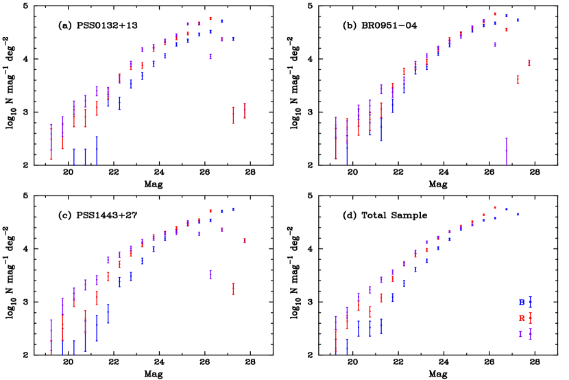
Figure 4: $BRI$ number count results for the three fields (a) PSS0132+13, (b) BR0951$-$04, (c) PSS1443+27, and (d) the entire sample. No corrections have been made for incompleteness although we have displayed only those counts of the total sample which we expect to have minor completeness corrections. Note that all of the magnitudes presented in this figure correspond to the Johnson-Cousins system.

4 PHOTOMETRY AND ASTROMETRY

The principal goal of this paper is to pre-select candidates at redshifts near $z_{abs}$ of the damped Ly$\alpha$ systems. We have chosen to survey $z\sim 4$ damped Ly$\alpha$ systems, therefore these galaxies will be significant $B$-dropouts. Because our imaging is more sensitive in $R$ than $I$, we first identified all candidates in the $R$ images with the software package SExtractor (v. 2.0.19). After experimenting with a negative image of BR0951$-$04, we determined that a 1.1$\sigma$ threshold and 6 pixel minimum area provided the largest number of candidates while minimizing spurious detections. For each field we created a SEGMENTATION map with SExtractor which identifies all of the significant object pixels in the image. We then used an in-house code to derive the magnitude and error of each object. The routine estimates the underlying sky flux by taking the biweight (Beers et al., 1990) of the sky in a circular annulus around each object containing at least 1000 pixels not flagged in the SEGMENTATION map. The errors in the magnitude measurements are derived from variance in the sky and object flux, and the uncertainty in the photometric calibration. The latter effect is a systematic error which aside from the color term is applied in the same way to every object. Magnitude measurements were repeated for the $B$ and $I$ filters restricting the apertures to the same set of pixels identified in the $R$ image. We determined that the seeing was sufficiently close between the various filters that a more sophisticated analysis was unwarranted. Many objects of interest are either weakly detected or undetected in the $B$ images. If these objects are bright enough for spectroscopy, they are essentially guaranteed to meet our $(B-R)_{AB}>2$ criterion. We are concerned primarily with the possibility of false positives, where these weakly detected objects are actually brighter than they appear due to a negative sky noise fluctuation and do not truly meet the $B-R$ criterion. Therefore, if the object flux is measured at $<3\sigma$ above the sky flux, we obtain a $1\sigma$ upper limit to the object flux by increasing its value by $1\sigma$ sky when the object flux is positive or simply setting it to $1\sigma$ sky when the object flux is negative. Finally, we estimated a corrected $I$ magnitude for each object using the MAG_ISOCOR routine in the SExtractor package. These corrected magnitudes were used to define our spectroscopic sample of $I_{AB}<25.5$. Finally, we performed accurate astrometry on each of our science fields to facilitate slit mask design. We implemented the coordinates routine kindly provided by J. Cohen to convert our LRIS $(x,y)$ pixel-coordinates to astrometric positions. We also identified stars from the USNO and HST Guide star catalogs in our images to determine a zero point in RA and DEC. An optimal USNO/HST star list had to be derived taking into account centroid inaccuracies of saturated stars and regions of distortion inherent to LRIS. The instrument’s true position angle relative to the sky was obtained using the companion routine pa_check. The position angles for PSS0132+1341, BR0951-0450, and PSS1443+2724 were found to be 180.0$\pm 0.46$, 180.1$\pm 0.25$, and 88.6$\pm 0.56$ degrees respectively. We estimate the error in the reported astrometric positions to be $\approx 1.0^{\prime\prime}$.

Tables 4–6 summarize the photometry and astrometry of all of the objects detected in at least one filter for the three fields. Columns 1$-$4 list the object positions: x-pixel, y-pixel, RA, DEC. Columns 5–10 the $BRI$ magnitudes and $1\sigma$ errors, Finally, column 11 provides the most likely photometric redshift, column 12 lists the best fit template, column 13 presents the confidence level for a $\Delta z=0.2$ interval centered at the most-likely redshift ($\S$ 5.3), and column 14 gives the probability that the object has $z\;\epsilon\;[3.5,4.5]$.

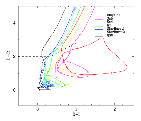
Figure 5: Model templates evolved from $z=0-7$ with steps of $\Delta z=0.5$ between symbols plotted in a $B-R$ vs. $R-I$ color diagram. The figure shows that only galaxies with $z>3.5$ lie within the selection region defined by the dashed lines; the first symbol within the selection region corresponds to $z=4$ for all templates. Therefore, this two color cut is an efficient means of pre-selecting high redshift galaxies.

5 RESULTS

5.1 Number Counts

We performed a number count analysis to provide a consistency check on our photometric calibration and analysis. We identified objects in each filter separately with the same approach used to select objects in $R$ for the $B$ drop-out analysis described in $\S$ 4, i.e. the SExtractor package implemented with a $1.1\sigma$ threshold and 6 pixel minimum area. We then measured isophotal and 1.5^′′ diameter aperture magnitudes for each object and adopted the brighter of the two. Note that these magnitudes may still underestimate the true magnitude as we have not considered isophotal or aperture corrections. We did not apply a color correction to any of the objects, but we did include the effects of Galactic extinction and airmass. Finally, we removed all objects with magnitude brighter than 22 which were identified by the SExtractor package as a star (i.e. CLASS_STAR $>0.8$). There may be a small but important stellar contribution to the counts in the magnitude $22-22.5$ bin, particularly in the $B$ filter.

Figure 4 presents the counts for the $BRI$ filters in each field and for the combined fields. These are raw counts only; no corrections for incompleteness have been applied. The magnitudes are on the $AB$ scale, the error bars assume $\sqrt{N}$ fluctuations and the bin size is 0.5 mag. While there is some variation from field to field, the differences are generally small. In panel (d) we plot the counts derived by combining the fields. To crudely account for incompleteness, we conservatively truncated the counts in each filter at the magnitude level where there is a significant ’turn over’ (e.g. I $\approx 25.5$ for PSS1443+25). We find that this criterion corresponds to $\approx 1$ mag brighter than the $3\sigma SB$ limits presented in Table 2, i.e. our true completeness limit for $z\sim 4$ galaxies is $\approx 1$ mag brighter than these $SB^{3\sigma}_{FWHM}$ values. Examining this panel, we observe results similar to those described by other number count studies (e.g. Steidel & Hamilton, 1993; Smail et al., 1995). In particular, the $B$ counts exhibit the steepest rise at $22-25$ mag with evidence for a flattening at fainter magnitudes. This bend in the slope is independent of completeness corrections because it occurs well above our detection limit. Meanwhile, the $R$ and $I$ slopes are nearly constant to the completeness limit. We note that the absolute scale of the number counts is lower than the Smail et al. (1995) results and expect the difference is due to the exact assumptions for apertures and corrected magnitudes. In summary, the number count data lend confidence to our photometric calibration and analysis.

5.2 Two-color Analysis

Steidel et al. (1999) were the first to demonstrate that one can efficiently pre-select $z\sim 4$ star-forming galaxies with broad band images. The approach is to design a set of color criteria which keys on the sharp flux decrement at the $\lambda\sim(1+z)\times 912$ Å Lyman break while also considering the substantial flux decrement due to absorption by intergalactic neutral hydrogen. The approach is well described by Figure 5 where we plot $(B-R)_{AB}$ vs. $(R-I)_{AB}$ colors for six galactic templates and one QSO template (see Yahata et al. 2000) adopting the quantum efficiencies of LRIS on the Keck telescope. The colored lines trace the evolutionary tracks of each template as they are $K$-corrected from $z=0$ to 5 and the points mark each $\Delta z=0.5$ interval. The dashed line demarcates the region of color-color space defining our selection criteria designed to include galaxies and the quasar with $z>3.5$ while minimizing the number of contaminating galaxies:

$$(B-R)_{AB}>2.0$$ (2)

$$(R-I)_{AB}<1.0$$ (3)

$$(B-R)_{AB}>1.2(R-I)_{AB}+1.6$$ (4)

These criteria follow the constraints imposed by Steidel et al. (1999) but were modified to account for our specific filter set. The large $B-R$ color criterion reflects the flux decrement due to the Lyman break and the Ly$\alpha$ absorption from intergalactic HI gas. In short, Figure 5 demonstrates that by restricting the objects to the upper left-hand corner of this color-color diagram we are sensitive to all galaxy types in the interval $3.5<z<4.5$ except those with rest-frame UV properties similar to Sab galaxies (i.e. galaxies with minimal ongoing star formation).

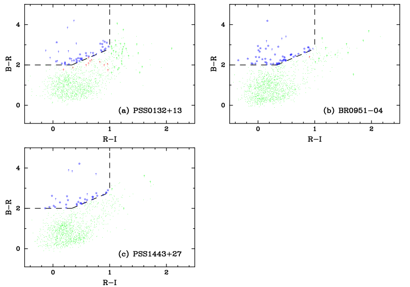
Figure 6: Two color diagram of all of the objects with a significant detection in the $R$ image. The blue stars and arrows are candidates which satisfy the selection criteria (designated by the dashed lines), the red arrows are galaxies with limits to their colors which might lie within the selection region, and the green points do not satisfy the criteria.

Figure 6 presents the color-color diagrams for all of the objects in the full exposure analysis regions of the three fields. As discussed in $\S$ 4, we selected objects and isophotal apertures in the $R$-band and then measured the $BRI$ magnitudes. In Figure 6 we have limited the objects to $I_{AB}<25.5$ which corresponds to an (ambitious) intrinsic spectroscopic limit set by a 2 hr integration time with LRIS on the Keck telescope. The dark blue points indicate objects which satisfy the color criteria, the red objects have a measured magnitude limit (typically in $B$) and might satisfy the criteria, and the green points are excluded from the selection region. In the case where we measure only a limit for a given color, we plot the point as an arrow. We visually inspected all candidate galaxies in our images and rejected roughly half of the initial candidates for having flawed photometry. The rejected candidates were typically near bright extended objects, satellite trails, or the borders of the images. It is no surprise that such a high fraction of the initial candidates had flawed photometry, as the color selection region is sparsely populated and therefore the small fraction of low-redshift galaxies scattered into the color selection region by photometric errors can easily comprise a large fraction of the candidates. Only a small fraction of the true high-redshift galaxies should be rejected during this step, although some of them may scatter out of the selection region due to photometric errors or unusual intrinsic colors. Bright (I$<23$) objects with clearly non-stellar morphology were rejected as low-redshift interlopers, but bright stellar objects were retained in case they were new quasars or lensing-magnified LBGs; most LBGs will look similar to point sources at the resolution of our images. The squares identify those candidates which were selected for follow-up multi-slit spectroscopy (see Paper II). For each field, $\sim 30-40$ objects lie within the selection region and an additional $\sim 10$ limits are consistent with the region. One can reliably construct a mask with 15$-$20 slits covering roughly half of the LRIS imaging field. Because some candidates conflict with others (particularly in the BR0951$-$04 field), we had the freedom to choose $\approx 5$ objects per mask which lie outside the selection region. The majority of these were chosen according to their photometric redshift. This explains why some objects in Figures 1-3 are marked as spectroscopic targets but not color dropouts.

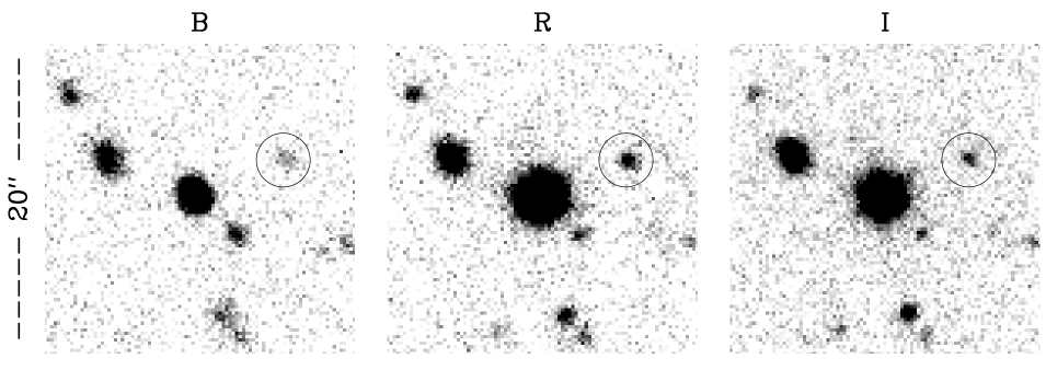
Figure 7: Close-up $BRI$ images ($20^{\prime\prime}\times 20^{\prime\prime}$) centered on the quasar PSS0132+13. The object identified to the right of the quasar is the only significant $B$-band dropout in this region and has a photometric redshift $z_{phot}=3.6$. The images are oriented with S up and E right.

5.3 Photometric Redshifts

Implementing the procedures introduced by Lanzetta et al. (1996) and Yahata et al. (2000), we have calculated photometric redshift likelihood functions for each object. The photometric redshift method accounts for the individual photometric uncertainties in the $B,R,$ and $I$ fluxes of each object and compares the object fluxes with a set of template spectra rather than a single two-color region. We adopted 6 galactic templates (elliptical, Sab, Scd, irregular, a reddened starburst, and an unreddened starburst), 1 quasar template, and $\sim$100 stellar templates with spectral type varying from O to M. We then stepped the non-stellar templates in 0.01 redshift intervals from $z=0$ to 7, identified the best fit template for each redshift, and recorded its $\chi^{2}$. Finally, we calculated the likelihood of the best fit template at each redshift interval to determine the most likely $z_{phot}$ value. As we are limited to only 3 filters per field, the confidence with which we can attribute a single redshift to a given object is often poor. For example, an object with $BRI$ magnitudes consistent with a $z=0.5$ elliptical galaxy is also well matched by a $z\approx 3.5$ Sab template. This degeneracy is revealed in Figure 5 at $B-R=2$ and $R-I=0.8$. In other words, essentially only those galaxies which satisfy the color-color criteria could be confidently identified as $z\sim 4$ galaxies. Therefore, in concordance with previous studies, we consider the selection region to be the most robust approach to efficiently identify a significant number of $z\sim 4$ galaxies in our fields.

In each of the fields, we identified a number of objects with $z_{phot}\sim 4$ that lie outside our color-color criteria. The majority of these galaxies were fit with early type spectra, not starburst models. We have included several of these candidates in the spectroscopic program in part to fill the slit masks (as noted above) but also to test the color-color criteria. In turn, we will better define our selection function for galaxies at $z\sim 4$. Preliminary results from Gawiser et al. (2001) indicate that with $BRI$ photometry alone, the photometric redshifts of galaxies confirmed spectroscopically to be at $3.5<z<4.5$ are quite accurate. However, a large number of low-redshift objects were aliased to high photometric redshifts due to color degeneracies between Lyman-break galaxies and low-redshift ellipticals (e.g. Steidel et al., 1999). The increased fraction of interlopers among candidates selected primarily by photometric redshift confirms that the color selection region modified from Steidel et al. (1999) is the most efficient place to find LBGs.

5.4 The Damped Ly$\alpha$ Systems

Figures 7–9 present 20${}^{\prime\prime}\times 20^{\prime\prime}$ $BRI$ images centered on the quasar of each field. At $z=4$, a $10^{\prime\prime}$ radius corresponds to 65 $h_{75}^{-1}$ kpc ($q_{0}=0.15,H_{0}=75h_{75}$ km/s/Mpc) which we expect encompasses the center of the galaxy giving rise to the damped Ly$\alpha$ system. For BR0951$-$04, there is a marginal $B$ drop-out ($B-R=1.7$) $\approx 7^{\prime\prime}$ below (North) the quasar. Its photometric redshift is $z_{phot}=3.7$ and its impact parameter corresponds to $\approx 50h^{-1}_{75}$ kpc. Although this separation would imply a very large gas disk in order to explain the observed ${N({\rm HI})}$ of either damped system, it can not be ruled out as the galaxy responsible for the absorption. There are no other significant $B$ drop-out candidates in this 20^′′ circle. Examining the PSS0132+13 field, we note a marginal $(B-R=1.5$) $B$ drop-out object $\approx 7^{\prime\prime}$ to the right (East) of PSS0132+13 with $z_{phot}=3.6$. Given the large separation and lower $B-R$ value, it is even less likely that this galaxy gives rise to the damped Ly$\alpha$ system. In contrast to the PSS0132+13 and BR0951$-$04 fields, the region surrounding PSS1443+27 is notably blank. In fact, there are only three significant galaxies in the 20${}^{\prime\prime}\times 20^{\prime\prime}$ area and only an additional 8 in a $30^{\prime\prime}\times 30^{\prime\prime}$ box, none of which are $B$-band dropouts. The absence of candidates is somewhat striking given that this system has the highest metallicity of any known $z>3$ damped Ly$\alpha$ system and might have been expected to exhibit an optical counterpart.

We have attempted to subtract the point-spread function (PSF) of the quasar to search for damped Ly$\alpha$ candidates underneath the PSF. We first used the software package (DAOPHOT) and IRAF routines to model the PSF of many bright stars throughout each field. We then focused on several stars close to the QSO to account for variations in the PSF across the field due to aberrations inherent to the LRIS imager. We then fit this PSF model to the quasar and subtracted it from the image. Unfortunately, owing to the segmented nature of the Keck telescope we found it too difficult to accurately model the PSF and had no success identifying objects underneath the PSF. Studies which take advantage of higher spatial resolution and a better behaved PSF (e.g. HST) are far more effective (e.g. Warren et al., 2001).

In summary, the only possible optical counterparts for the four damped Ly$\alpha$ systems down to $I_{AB}<25.5$ lie at impact parameter $\approx 7^{\prime\prime}$ from the sightline. This is a significant separation even without considering projection. We expect – if anything – that these galaxies are clustered with the damped Ly$\alpha$ system. If we assume that at least one of the galaxies giving rise to the damped Ly$\alpha$ systems does not lie beneath the PSF of the quasar (Warren et al., 2001), then we can place an upper limit to its luminosity based on the depth of our $I$ images. At $z=4$, Steidel et al. (1999) have fit a Schechter luminosity function to their sample of Lyman break galaxies and find $L^{*}_{LBG}$ corresponds to $I_{AB}\approx 25$ mag. For the PSS0132+13 and PSS1443+27 fields, where no reasonable candidate was identified in the images, our $3\sigma$ limits in the $I$-band of 27.4 and 26.6 correspond to $L<L_{LBG}^{*}/9$ and $L_{LBG}^{*}/4$ respectively.

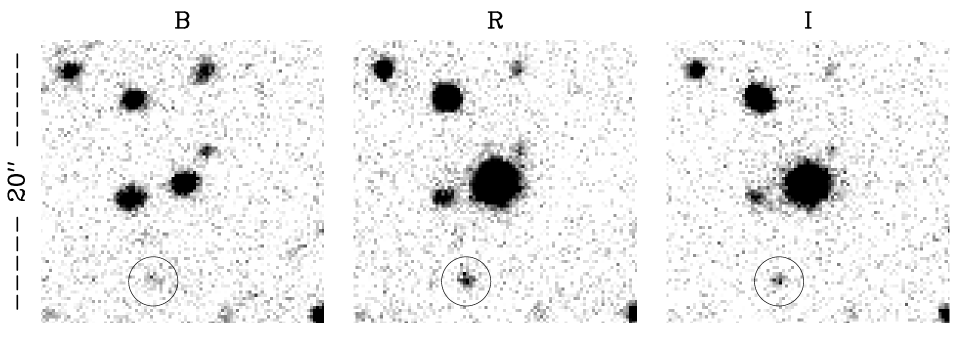
Figure 8: Close-up $BRI$ images ($20^{\prime\prime}\times 20^{\prime\prime}$) centered on the quasar BR0951$-$04. The marked object below the quasar is the only significant $B$-band dropout in this region and has a photometric redshift $z_{phot}=3.7$. The images are oriented with S up and E right.

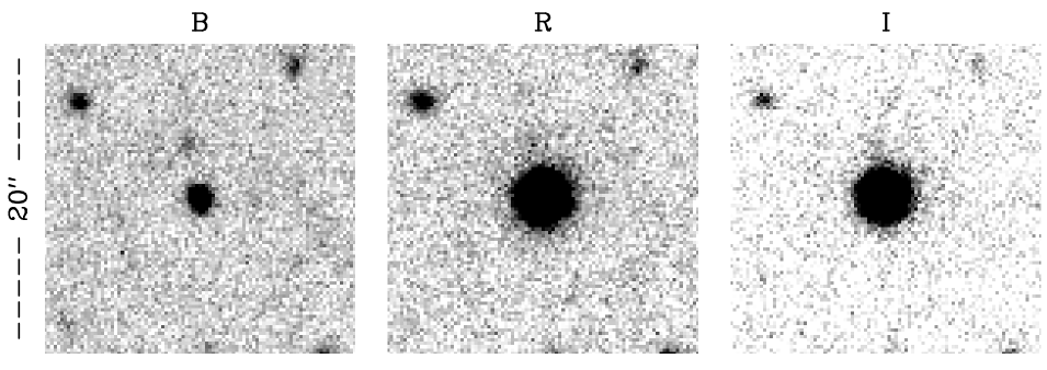
Figure 9: Close-up $BRI$ images ($20^{\prime\prime}\times 20^{\prime\prime}$) centered on the quasar PSS1443+27. Unlike the other two fields, there is not a single significant $B$-band dropout in this region. In fact, there are an unusually small number of galaxies of any type near the quasar. The images are oriented with E up and N right.

6 SUMMARY

We have presented an analysis of $BRI$ images for three fields containing quasars with four known damped Ly$\alpha$ systems at $z\sim 4$. The data was reduced with standard procedures and calibrated with Landolt standard stars taken close to the time of the observations. We measured $BRI$ magnitudes for all of the objects in each field using isophotal apertures and measured $B-R$ and $R-I$ colors for those galaxies detected in the $R$-images. A rough number count analysis agrees well with other studies in the literature to similar magnitude limits.

By searching for $B$-band dropouts and measuring photometric redshifts, we have culled a list of candidates at $z\sim 4$ throughout each field for follow-up spectroscopy. We identified $\approx 30-40$ candidates per field to a limiting magnitude of $I_{AB}<25.5$. For the three fields there are only two dropouts detected within $10^{\prime\prime}$ of the quasar, each at an impact parameter of $\approx 7^{\prime\prime}$. Although these two galaxies could give rise to one or two of the damped Ly$\alpha$ systems, we expect it is more likely that they are either clustered with the damped system or at a different redshift altogether. Therefore, we have no convincing detections of the galaxy in emission for four damped systems in the three fields. Either the galaxies are fainter than our detection limit ($\approx L_{LBG}^{*}/4$) or located under the PSF of the background quasar. Nevertheless, our results enable a study of the large-scale clustering of galaxies associated with the damped Ly$\alpha$ systems. Indeed, this is the focus of the analyses presented in companion papers (Paper II).

References

- Adelberger et al. (1998) Adelberger, K. L., Steidel, C.C., Giavalisco, M., Dickinson, M., Pettini, M., & Kellogg, M. 1998, ApJ, 505, 18
- Beers et al. (1990) Beers, T.C., Flynn, K., & Gebhardt, K. 1990, AJ, 100, 32
- Bessel (1983) Bessel, M.S. 1983, PASP, 95, 480
- Djorgovski et al. (1996) Djorgovski, S.G., Pahre, M.A., Bechtold, J., & Elston, R. 1996, Nature, 382, 234
- Djorgovski (1997) Djorgovski, S.G. 1997, astro-ph/9709001
- Fukugita et al. (1996) Fukugita, M., Ichikawa, T., Gunn, J.E., Doi, M., Shimasku, K., & Schneider, D.P. 1996, AJ, 111, 1748
- Gawiser et al. (2001) Gawiser, E., Wolfe, A.M., Prochaska, J.X., Lanzetta, K.M., Yahata, N., & Quirrenbach, A. 2001, ApJ, 562, 628
- Gawiser et al. (2002) Gawiser, E., et al. 2002, in preparation
- Hu et al. (1998) Hu, E.M., Cowie, L.L., McMahon, R.G. 1998, ApJ, 502, 99L
- Kauffmann (1996) Kauffmann, G. 1996, MNRAS, 281, 475
- Landolt (1992) Landolt, A.U. 1992, AJ, 104, 340
- Lanzetta et al. (1996) Lanzetta, K.M., Yahil, A., & Fernandez-Soto, A. 1996, Nature, 381, 759
- Madau (1995) Madau, P. 1995, ApJ, 441, 18
- Oke et al. (1994) Oke, J.B., Cohen, J.G., Carr, M., Dingizian, A., Harris, F.H., Lucinio, R., Labrecque, S., Schaal, W., & Southard, S. 1994, SPIE, 2198, 178
- Prochaska & Wolfe (1997a) Prochaska, J. X. & Wolfe, A. M. 1997, ApJ, 474, 140
- Prochaska & Wolfe (1999) Prochaska, J.X. & Wolfe, A.M., 1999, ApJS, 121, 369
- Prochaska & Wolfe (2000) Prochaska, J.X. & Wolfe, A.M., 2000, ApJ, 533, L5
- Prochaska et al. (2001) Prochaska, J.X., Wolfe, A.M., Tytler, D., Burles, S.M., Cooke, J., Gawiser, E., Kirkman, D., O’Meara, J.M., & Storrie-Lombardi, L. 2001, ApJS, 137, 21
- Schlegel et al. (1998) Schlegel, D.J., Finkbeiner, D.P., & Davis, M. 1998, ApJ, 500, 525
- Smail et al. (1995) Smail, I., Hogg, D.W., Yan, L., & Cohen, J. 1995, ApJ, 449 105
- Steidel & Hamilton (1993) Steidel, C.C., & Hamilton, D. 1993, AJ, 105, 2017
- Steidel et al. (1999) Steidel, C.C., Adelberger, K., Giavalisco, M., Dickinson, M., & Pettini, M., 1999, ApJ, 519, 1
- Storrie-Lombardi et al. (1996) Storrie-Lombardi, L.J., Irwin, M.J. 1996, & McMahon, R.G. MNRAS, 282, 1330
- Storrie-Lombardi and Wolfe (2000) Storrie-Lombardi, L.J. & Wolfe, A.M. 2000, ApJ, 543, 552
- Vogt et al. (1994) Vogt, S.S., Allen, S.L., Bigelow, B.C., Bresee, L., Brown, B., et al. 1994, SPIE, 2198, 362
- Warren et al. (2001) Warren, S.J., Moller, P., Fall, S.M., & Jakobsen, P. 2001, MNRAS, 326, 759
- Wolfe et al. (1986) Wolfe, A.M., Turnshek, D.A., Smith, H.E., & Cohen, R.D. 1986, ApJS, 61, 249
- Yahata et al. (2000) Yahata, N., Lanzetta, K.M., Chen, H.-W., Fernández-Soto, A., Pascarelle, S.M., Yahil, A., & Puetter, R.C. 2000, ApJ, 538, 493