Abstract

We show that the astrometric Hipparcos data of the stars hosting planet candidates are not accurate enough to yield statistically significant orbits. Therefore, the recent suggestion, based on the analysis of the Hipparcos data, that the orbits of the sample of planet candidates are not randomly oriented in space, is not supported by the data. Assuming random orientation, we derive the mass distribution of the planet candidates and shows that it is flat in log M, up to about 10 $M_{Jup}$. Furthermore, the mass distribution of the planet candidates is well separated from the mass distribution of the low-mass companions by the ’brown-dwarf desert’. This indicates that we have here two distinct populations, one which we identify as the giant planets and the other as stellar secondaries. We compare the period and eccentricity distributions of the two populations and find them surprisingly similar. The period distributions between 10 and 1650 days are flat in log period, indicating a scale-free formation mechanism in both populations. We further show that the eccentricity distributions are similar — both have a density distribution peak at about 0.2–0.4, with some small differences on both ends of the eccentricity range. We present a toy model to mimic both distributions. The toy model is composed of Gaussian radial and tangential velocity scatters added to a sample of circular Keplerian companions. A scatter of a dissipative nature can mimic the distribution of the eccentricity of the planets, while scatter of a more chaotic nature could mimic the secondary eccentricity distribution. We found a significant paucity of massive giant planets with short orbital periods. The low-frequency of planets is noticeable for masses larger than about 1 $M_{Jup}$ and periods shorter than 30 days. We point out how, in principle, one can account for this paucity.

1 Introduction

More than fifty candidates for extrasolar planets have been announced over the past six years (e.g., Schneider 2001). In each case, precise stellar radial-velocity measurements indicated the presence of a low-mass unseen companion, with a minimum mass between 1 and about 10 Jupiter masses ($M_{Jup}$). The identification of these unseen companions as planets relied on their masses being in the planetary range.

However, the actual masses of the planet candidates are not known. The radial-velocity data yield only $M_{2}\sin\,i$, where $M_{2}$ is the secondary mass and $i$ is the inclination angle of its orbital plane, which cannot be derived from the spectroscopic data. Nevertheless, the astronomical community considered the planet-candidate masses as being close to their derived minimum masses — $M_{2}\sin\,i$. This is so because at random orientation the most probable inclination is $90^{\circ}$, and the expected value of $\sin\,i$ is close to unity.

Very recently some doubt has been cast about the validity of the random orientation assumption. Gatewood, Han, & Black (2001) and Han, Black, & Gatewood (2001) analysed the Hipparcos astrometric data of the stars hosting planet candidates together with the stellar precise radial-velocity measurements and derived in some cases very low inclination angles for the orbital planes. Han, Black, & Gatewood (2001) found eight out of 30 systems with an inclination smaller or equal to $0.5^{\circ}$, four of which they categorized as highly significant. The probability of finding such small inclinations in a sample of orbits that are isotropically oriented in space is extremely small, indicating either a problematic derivation of the astrometric orbit, or, as suggested by Han, Black, & Gatewood (2001), some serious orientation bias in the inclination distribution of the sample of detected planet candidates.

However, the analysis of the Hipparcos data can be misleading. As has been shown by Halbwachs et al. (2000), one can derive a small false orbit with the size of the typical positional error of Hipparcos, about 1 milli-arc-second (=$mas$), caused by the scatter of the individual measurements. Therefore, one should carefully evaluate the statistical significance of any astrometric orbit of that size derived from the Hipparcos data. In Section 2 we summarize our work (Zucker & Mazeh 2001a) that evaluates the significance of the astrometric orbits by applying a permutation test to the Hipparcos data. Similarly to the results of Pourbaix (2001) and Pourbaix & Arenou (2001), we also find that the significance of all the Hipparcos astrometric orbits of the planet candidates are less than 99%, including $\rho$ CrB that attracted much attention after the publication of Gatewood, Han, & Black (2001) suggestion. We therefore conclude that the Hipparcos data does not prove the anisotropy of the orientations of the orbital planes of the planet candidates.

After showing that the random orientation in space is still a reasonable assumption, not confronted by any available measurement, we present in Section 3 our work (Zucker & Mazeh 2001b) that uses this assumption to derive the mass distribution of the planet candidates. This is done with MAXLIMA, a MAXimum LIkelihood MAss algorithm which we constructed to derive the mass distribution. Similar to the results of Jorrisen, Mayor & Udry (2001), we show that the mass distribution of the planet candidates is separated from the one of the secondary masses by the so-called ’brown-dwarf desert’ (e.g., Marcy & Butler 2000). This indicates that we are dealing with two different classes of objects. One is the giant planets, with masses not far from the planetary mass range, while the other is the low-mass secondaries, with stellar mass range.

One could speculate that the separation between the two different mass distributions indicates different formation processes. The commonly accepted paradigm is that planets were probably formed by coagulation of smaller, possibly rocky, bodies, whereas stars were probably formed by some kind of fragmentation of larger bodies. In other words, planets were formed by small bodies that grew larger, whereas stars, binary included, were formed by fragmentation of large bodies into smaller objects (e.g., Lissauer 1993; Black 1995). This could imply, for example, that the distribution of orbital eccentricities of giant planets and low-mass binaries would be substantially different. All the solar planets have nearly circular orbits, whereas binaries have eccentric orbits (e.g., Mazeh, Mayor, & Latham 1996). We could also expect the periods of planets to be longer than 10 years, like the giant planets in the solar system. Many studies of the newly discovered planets showed that this is not the case (e.g., Marcy, Cochran, & Mayor 2000). Moreover, following Heacox (1999) who based his analysis upon only 15 binaries and a handful of planet candidates, we show in Section 4 that within some reasonable restrictions, the eccentricity and period distributions of the two samples are surprisingly similar. Similar results have been obtained by Stepinski & Black (2001a,b,c). In Section 5 we consider a toy model that can generate the eccentricity distribution of both populations.

2 The Significance of the Astrometric Orbits

In this section we present our work (Zucker & Mazeh 2001a) where we evaluate for each of the extrasolar planets the statistical significance of its astrometric orbit, derived from the Hipparcos data together with its radial-velocity measurements. We first derived the best-fit orbit by assuming that the spectroscopic and astrometric solutions have in common the following elements: the period, $P$, the time of periastron passage, the eccentricity, $e$, and the longitude of the periastron. In addition, the spectroscopic elements include the radial-velocity amplitude, $K$, and the center-of-mass radial velocity. We have three additional astrometric elements — the angular semi-major axis of the photocenter, $a_{0}$, the inclination, $i$, and the longitude of the nodes. In addition, the astrometric solution includes the regular astrometric parameters — the parallax, the position and the proper motion.

In most cases the elements are not all independent. From the spectroscopic elements we can derive the projected semi-major axis of the primary orbit. This element, together with the inclination $i$ and the parallax, yields the angular semi-major axis of the primary, $a_{1}$. Assuming the secondary contribution to the total light of the system is negligible, this is equal to the observed $a_{0}$.

To find the statistical significance of the derived astrometric orbit in each case we applied a permutation test (e.g., Good 1994) to the Hipparcos data. For each star we generated simulated permuted astrometric data and analyzed them either together with the actual individual radial velocities of that star, or by imposing the published spectroscopic elements. Details of the analysis are given by Zucker & Mazeh (2001a).

The distribution of the falsely detected semi-major axes indicated the range of possible false detections. For example, $a_{99}$ — the 99-th percentile, denotes the semi-major axis size for which 99% of the simulations yielded smaller values. Consequently, an astrometric orbit is detected with a significance of 99% if and only if the actually derived semi-major axis, $a_{derived}$, is larger than $a_{99}$.

As an illustration, Figure 1A shows the histogram of the semi-major axis derived by random permutations of the Hipparcos data of HD 209458. This star’s inclination is known to be close to $90^{\circ}$ through the combination of radial velocity and transit measurements (Charbonneau et al. 2000; Mazeh et al. 2000; Henry et al. 2000; Brown et al. 2001). The Hipparcos derived semi-major axis, $a_{derived}$, is 1.76 $mas$, which is marked in the figure by an arrow. One can clearly see that many random permutations led to larger semi-major axes, a fact that renders this derived value insignificant. The derived value is obviously false since the known inclination implies a value of less than a micro-arc-second.

In Figure 1B we show an opposite case, HD 164427, where the derived astrometric orbit is quite significant. Note that $a_{derived}$ is relatively large — 3.11 $mas$, which made the significant detection possible. However, this is not a planet-candidate case. The minimum mass suggests this secondary is a brown-dwarf candidate, whereas the astrometric orbit shows the secondary mass is in the stellar regime.

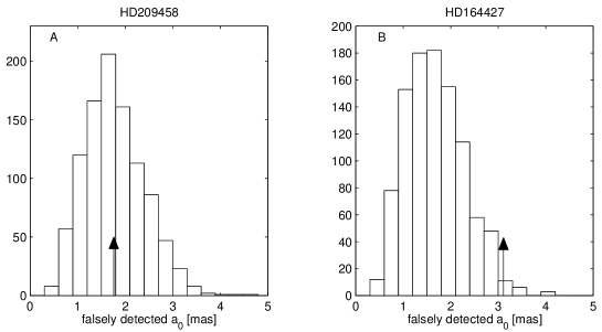
Figure 1: Histograms of the size of the falsely derived semi-major axes in the simulated permuted data of HD 209458 (A) and HD 164427 (B). The size of the actually detected axes are marked by an arrow.

As of March 2001, the Encyclopedia of extrasolar planets included 49 planet candidates with minimum masses smaller than 13 $M_{Jup}$. We (Zucker & Mazeh 2001a) analyzed all but two of the planet candidates. One star had no Hipparcos data, and the other star is known to have two companions. Figure 2 presents our results by depicting $a_{derived}$ versus $a_{99}$. The figure indeed shows that all points fall to the right of the line $a_{derived}=a_{99}$. This means that all our derived astrometric motions are not significant in the 99% level. This includes the planets of $\upsilon$ And and HD 10697 whose derived orbits were previously published by us (Mazeh et al. 1999; Zucker & Mazeh 2000), but the new analysis renders their orbits less significant.

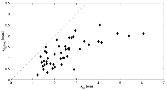
Figure 2: The derived semi-major axes of the planet candidates as a function of the 99-th percentile of the falsely derived semi-major axes. The dashed line represents the line $a_{derived}=a_{99}$.

Note, however, that this does not mean that the orbits derived are all false. Figure 2 shows that some of the systems are close to the border line, indicating that the orbits of these systems were detected with significance close to 99%. The systems with significance higher than 90% are listed in Table 1. Here we list the Hipparcos number and the stellar name, the confidence level of the derived astrometric orbit, the derived semi-major axis, its uncertainty and the derived inclination; the derived secondary mass together with its 1$\sigma$ range.

HIP	Name	Signif-	$a_{derived}$	$\sigma_{a}$	$i_{derived}$	$M_{derived}$	Mass Range
number		icance	($mas$)	($mas$)	(deg)	($M_{\odot}$)	(1$\sigma$)
5054	HD 6434	0.96	1.34	0.67	-0.08	0.45	(0.20,0.77)
43177	HD 75289	0.90	1.05	0.52	0.03	1.13	(0.45,2.19)
78459	$\rho$ CrB	0.98	1.49	0.46	0.54	0.12	(0.086,0.17)
90485	HD 169830	0.92	1.25	0.64	2.1	0.081	(0.039,0.124)
94645	HD 179949	0.90	1.92	0.68	0.034	3.4	(1.57,6.49)
98714	HD 190228	0.95	1.82	0.77	4.5	0.064	(0.037,0.093)
100970	HD 195019	0.92	2.24	0.78	0.32	0.92	(0.51,1.47)

Table 1: Derived planet-candidate orbits with confidence level higher than 90%.

To summarize, the combination of the Hipparcos data together with the radial-velocity measurements did not yield any astrometric orbit with significance higher than 99%. Apparently, the Hipparcos precision is not good enough to detect a 1 $mas$ orbit, even with the combination of the radial-velocity measurements. The analysis shows that the data are consistent with no astrometric detection at all, although one or two true astrometric orbits, which imply low inclinations, are still possible. However, such a finding would not prove that the orbits of the sample of planet candidates are not randomly oriented in space.

3 The Mass Distribution of the Extrasolar Planets

Assuming the orbits of the detected planet candidates are randomly oriented in space we can now proceed to derive their mass distribution. To do that we have to account for the unknown orbital inclination and for the fact that stars with too small radial-velocity amplitudes could not have been detected as radial-velocity variables. Therefore, planets with masses too small, orbital periods too large, or inclination angles too small were not detected.

Numerous studies accounted for the effect of the unknown inclination of spectroscopic binaries (e.g., Mazeh & Goldberg 1992; Heacox 1995; Goldberg 2000), assuming random orientation in space. Heacox (1995) calculated first the minimum-mass distribution and then used its relation to the actual mass distribution to derive the latter. This calculation amplified the noise in the observed data, and necessitated the use of quite heavy smoothing of the observed data. Mazeh & Goldberg (1992) introduced an iterative algorithm whose solution depended, in principle, on the initial guess.

Very recently Jorissen, Mayor, & Udry (2001a) studied the planet distribution by considering only the effect of the unknown inclination. Like Heacox (1995), Jorrisen, Mayor, & Udry derived first the distribution of the minimum masses and then applied two alternative algorithms to invert it to the distribution of planet masses. One algorithm was a formal solution of an Abel integral equation and the other was the Richardson-Lucy algorithm (e.g., Heacox 1995). The first algorithm necessitated some degree of data smoothing and the second one required a series of iterations. The results of the first algorithm depended on the degree of smoothing applied, and those of the second one on the number of iterations performed. In addition, Jorissen, Mayor, & Udry (2001) did not apply any correction to the observational selection effect.

We (Zucker & Mazeh 2001b) followed Tokovinin (1991, 1992) and constructed a maximum likelihood algorithm — MAXimum LIkelihood MAss, to derive an histogram of the mass distribution of the extrasolar planets. MAXLIMA derives the histogram directly by solving a set of numerically stable linear equations. It does not require any smoothing of the data, except for the bin size of the histogram, nor any iterative procedure. MAXLIMA also offers a natural way to correct for the undetected planets. This is done by considering each of the detected systems as representing more than one system with the same $M_{2}\sin\,i$, depending mainly on the period distribution. The details of the algorithm are given in Zucker & Mazeh (2001b).

To apply MAXLIMA to the current known sample of extrasolar planets we (Zucker & Mazeh 2001b) considered all known planets and brown dwarfs orbiting G- or K-star primaries as of April 2001. To acquire some degree of completeness to our sample we have decided to exclude planets with periods longer than 1500 days and with radial-velocity amplitudes smaller than 40 m/s. The values of these two parameters determine the correction of MAXLIMA for the selection effect, for which we assumed a period distribution which is flat in $\log P$. This choice of parameters also implies that our analysis applies only to planets with periods shorter than 1500 days. We further assumed that the primary mass is 1$M_{\odot}$ for all systems.

The results of MAXLIMA are presented in the lower panel of Figure 3 on a logarithmic mass scale. The value of each bin is proportional to the estimated number of planets found in the corresponding range of masses in the known sample of planet candidates, after correcting for the undetected systems. To estimate the uncertainty of each bin we ran 5000 Monte Carlo simulations and found the r.m.s. of the derived values of each bin. Therefore, the errors plotted in the figure represent only the statistical noise of the sample. Obviously, any deviation from the assumptions of our model for the selection effect induces further errors into the histogram, the assumed period distribution in particular. This is specially true for the first bin, where the actual number of systems is small and the correction factor large.

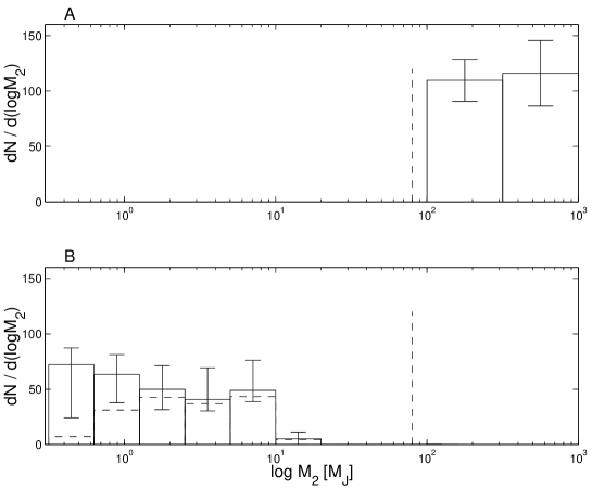
Figure 3: The mass distributions of the planets (lower panel) and the stellar companions (upper panel). The horizontal dashed lines represent the mass distribution without the correction for the selection effect. The vertical dashed line marks the stellar–sub-stellar border line.

To compare the mass distribution of the planet candidates with that of the stellar secondaries we plot (Zucker & Mazeh 2001b) the latter on the same scale in an adjacent panel of Figure 3. We plot here only two bins, with masses between 100 and 1000 $M_{Jup}$, using subsamples of binaries found by the Center for Astrophysics (=CfA) radial-velocity search for spectroscopic binaries (Latham 1985) in the Carney & Latham (1987) sample of the high-proper-motion stars (Latham et al. 2001; Goldberg et al. 2001).

Note that the upper panel does not have any estimate of the values of the bins with masses smaller than 100 $M_{Jup}$. This is so because the CfA search does not have the sensitivity to detect secondaries in that range. On the other hand, the lower panel does include information on the bins below 100 $M_{Jup}$. This panel presents the results of the high-precision radial-velocity searches, and these searches could easily detect stars with secondaries in the range of, say, 20–100 $M_{Jup}$. The lower panel shows that the frequency of secondaries in this range of masses is close to zero.

The relative scaling of the planets and the stellar companions is not well known (see Zucker & Mazeh 2001b for a detailed discussion). Nevertheless the comparison is illuminating. It suggests that we have here two distinct populations, separated by a ’gap’ of about one decade of masses, in the range between 10 and 100 $M_{Jup}$. We will assume that the two populations are the giant planets, at the low-mass side of Figure 3, and the stellar companions at the high-mass end of the figure. The present analysis is not able to tell whether the gap extends up to 60, 80 or 100 $M_{Jup}$.

The gap between the two populations was already noticed by many previous studies (Basri & Marcy 1997; Mayor, Queloz, & Udry 1998; Mayor, Udry, & Queloz 1998; Marcy & Butler 1998). Those papers binned the mass distribution linearly. Here we follow our previous work (Mazeh, Goldberg & Latham 1998; Mazeh 1999a,b; Mazeh & Zucker 2001) and use a logarithmic scale to study the mass distribution, because of the large range of masses, 0.5–1000 $M_{Jup}$, involved. The gap or the brown-dwarf desert is consistent also with the finding of Halbwachs et al. (2000), who used Hipparcos data and found that many of the known brown-dwarf candidates are actually stellar companions.

The distribution we derived in Figure 3 suggests that the planet mass distribution is almost flat in $\log M$ over five bins — from 0.3 to 10 $M_{Jup}$. Actually, the figure suggests a possible slight rise of the distribution toward smaller masses. At the high-mass end of the planet distribution the mass distribution dramatically drops off at 10 $M_{Jup}$, with a small high-end tail in the next bin. Although the results are still consistent with zero, we feel that the small value beyond 10 $M_{Jup}$ might be real. The dramatic drop at 10 $M_{Jup}$ and the small high-mass tail agree with the findings of Jorissen, Mayor, & Udry (2001), despite the differences in the algorithm used to derive the distribution, and the logarithmic scale we use for the distribution.

4 Eccentricity and Period Distribution of the Two Populations

Having established the difference between the mass distribution of the giant planets and that of the low-mass secondaries in spectroscopic binaries, we turn now to compare the period and eccentricity distributions of the two populations. For the latter we use (Mazeh & Zucker 2001) the results of a very large radial-velocity study of the Carney & Latham (1987) high-proper-motion sample, which yielded about 200 spectroscopic binaries (Latham et al. 2001; Goldberg et al. 2001). Goldberg (2000) separated statistically between the binaries of the Galactic halo and those coming from the disk. We consider in this section only the 59 single-lined spectroscopic binaries (=SB1s) of the Galactic disk. For the giant planet sample we use again the sample of 66 planet candidates listed in Schneider (2001) as of April 2001.

Figure 4A shows the cumulative period distribution of the two samples. The figure suggests similar general trend, except in the two ends of the distributions. We therefore plotted in Figure 4B the two distributions only in the range between 10 and 1650 days. The similarity is astounding, since the two distributions are identical. Both are consistent with a straight line, which implies a flat distribution in log P.

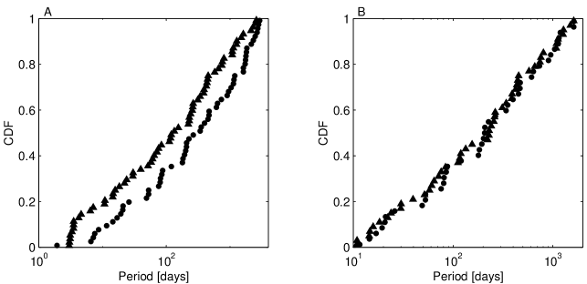
Figure 4: The period cumulative distribution for the planet candidates (triangles) and the Galactic disk SB1s (circles). A. All the stars in the samples. B. After restricting the samples to $10<P<1560\,{\rm d}$.

We speculate that at the short period range, below 10 days, some dynamical interaction changed the distribution of either one or both distributions. Such an interaction could also change the eccentricity distribution of the orbits. In order not to be distracted by this possible interaction when we consider the eccentricity distribution, we choose to consider only the eccentricities of the orbits with periods between 10 and 1650 days. The cumulative distributions are plotted in Figure 5A. We again see a similar trend in both distributions, except in both ends of the range [0,1]. To illuminate the difference we plotted the density distribution in Figure 5B. We derived the distribution by convolving the actual data points with a Gaussian kernel with a width of 0.08. It is clear that both distributions peak at about 0.2–0.4. However, the distribution of the spectroscopic binaries drops sharply toward zero, whereas the planet distribution does not. The eccentricity distribution of the binaries displays a tentative ’shoulder’ at the large eccentricities, whereas that of the planets displays such a possible shoulder at the small eccentricities.

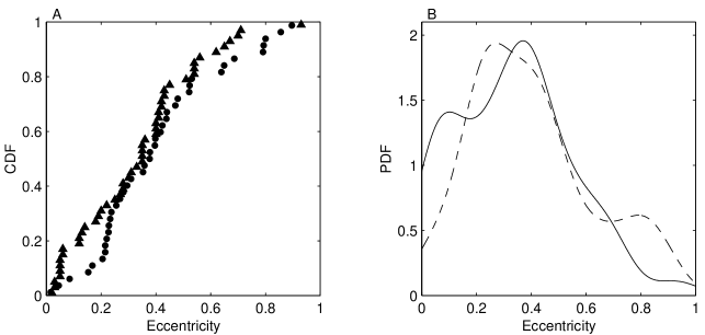
Figure 5: A. The eccentricity cumulative distribution for the planet candidates (triangles) and the Galactic disk SB1s (circles), restricted to $10<P<1560\,{\rm d}$. B. Estimated probability density function of the same samples, using a 0.08-wide kernel. The continuous line represents the planets and the dashed line represents the SB1s.

Any paradigm that assumes the two populations were formed differently has to explain why their eccentricity as well as period distributions are so much alike. Although we do not try to explain any of the two similarities, we suggest in the next section a toy model that can generate the two eccentricity distributions.

5 A Toy Model to Generate the Eccentricity Distributions of the Two Samples

Consider a sample of low-mass companions that orbit their parent stars in circular Keplerian orbits. For simplicity let us choose the units such that the orbital radii of all orbits are of length unity, and so are their orbital tangential velocities. Now let us introduce a Gaussian scatter to the velocities of the companions of the sample, with two independent components. One component is tangential and the other is radial. The tangential component changes the moduli of the velocities, while the radial one changes mainly their directions.

The new scatter determined the new velocity distribution. Denote the center of the distribution by $v_{0}$ and its r.m.s. by $\sigma_{v}$. Suppose that the velocity angles are distributed around $90^{\circ}$, with r.m.s of $\sigma_{\theta}$. Note that the distribution has three parameters, $v_{0}$, $\sigma_{v}$ and $\sigma_{\theta}$.

We can now calculate the eccentricity distribution of the sample, and see if such a simple-minded toy model can mimic the observed distributions of the giant planets and the low-mass companions. Figure 6 compares the two. We found that we can approximate the giant planet distribution with $v_{0}=0.82$ and $\sigma_{v}=0.13$, while $\sigma_{\theta}=0$, whereas the low-mass stellar companions necessitated $\sigma_{\theta}=25^{\circ}$, $\sigma_{v}=0.05$ and $v_{0}=1.08$.

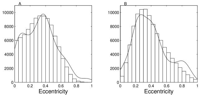
Figure 6: The simulated eccentricities histograms, together with the empirically estimated distributions of the planet candidates (A) and the stellar companions (B).

The fact that we succeeded to mimic the two actual distributions is not surprising. As the old statistical saying goes: “You can fit an elephant with any model with two parameters, and you can make him dance with three”. However, the specific values of the parameters found are somewhat intriguing. Suppose that both populations started with Keplerian circular orbits, and two mechanisms introduced the scatter into the two populations. Suppose the nature of the mechanism that operated on the planet population was dissipative, like the dissipation generated by an interaction of a planet with a swarm of small particles in a disk. Such a mechanism could decrease the velocity without changing its direction. This would result with a null $\sigma_{\theta}$ and $v_{0}$ less than unity, the difference being of the same order of $\sigma_{v}$. On the other hand, the spectroscopic binaries could be subject to a more chaotic, eruptive disturbing mechanism, like the gravitational interaction with a few large bodies. In such a process one could expect a spread of the velocity directions and moduli, without significantly changing $v_{0}$. This simple-minded picture is consistent with our findings.

We should emphasize that the aforementioned discussion is not meant to explain how the eccentricities were formed, nor why the two distributions are similar with some definite small differences. The model might only serve as a starting point for any theoretical study to account for the observed distributions.

6 The Paucity of Short-Period Massive Planets

In Section 3 & 4 we have discussed the distributions of masses, periods and eccentricities of the extrasolar planets. In this section we move to examine one aspect of the inter dependence of these variables. To explore this possible dependence we performed a Principal Component Analysis (e.g., Kendall & Stuart 1958), which immediately pointed out to the significant correlation between the (minimum) masses and periods of the extrasolar planets. This is depicted in Figure 7, in which we plotted the period as a function of the (minimum) masses of the known planets, as of April 2001. We choose to plot the two axes with logarithmic scales, because the frequency of planets is flat in log M and log P, as has been shown in previous sections.

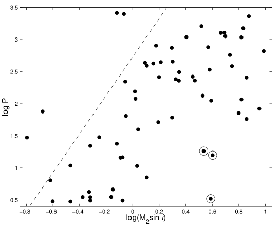
Figure 7: The logarithm of the period vs. the logarithm of the mass of the planet candidates. The dashed line represents a detection limit of 25 m s^-1 radial velocity amplitude. The three circled points correspond to the stars HD 195019, Gls 86 and $\tau$ Boo (see text).

Most of the correlation between the periods and masses of the extrasolar planets could be accounted for by a selection effect, that prevents planets which are not massive enough from being discovered if their periods are too long. Such systems have radial-velocity amplitude, $K$, which is too small to be detected by the present planet-search projects. This is easily seen in the small-mass–long-period corner of the diagram, bounded by the $K=25\,{\rm m\thinspace s^{-1}}$ line. There are only four planets above this line. However, a close examination of Figure 7 reveals an additional feature — a significant paucity of planets at the opposite, large-mass–short-period corner of the diagram. Only three planets appear at that corner, all marked by a circle. This is certainly not a selection effect, because planets at that part of the diagram have the largest radial-velocity amplitude, and therefore are the easiest to detect.

It is not clear yet what is the shape of the area in which we find low frequency of planets. That corner might have a rectangular shape bordered by $\log(M_{2}\sin i)=0.2$ and $\log P=1.5$, or could be of a wedge shape, bordered by the line that goes from $\Large(\log(M_{2}\sin i),\log P\Large)=(0,0.5)$ to $(1,1.5)$.

The three planets that we find in the small-mass–long-period corner are Gls 86, HD 195019 and $\tau$ Boo. Interestingly enough, all three systems are wide binaries. Els et al. (2001) discovered very recently that the star Gls 86 has a brown-dwarf companion at about 20 AU projected separation. Pourbaix & Arenou (2001) pointed out that HD 195019 is a known visual binary with a companion fainter by about 3 mag., observed at a separation of 3.5 arc-sec in 1988 (Mason et al. 2001). The angular separation of HD 195019 (=WDS 20283+1846) translates to 130 AU projected separation for a parallax of 27 $mas$ (ESA 1997). The third star, $\tau$ Boo, is also a known visual binary (WDS 13473+1727), with an M2 companion. Apparently, the period is about two thousand years (Hale 1994) and the orbit is very eccentric. The separation between the two stars has been measured in 1991 to be 3.4 arc-sec (Mason et al. 2001), which translates to about 50 AU projected distance for a parallax of 64 $mas$ (ESA 1997). Planets in binary systems might go through different orbital evolution, and therefore might be considered as special cases. Thus, the low frequency of planets with large masses and short periods seems to be even more real than is seen from the figure.

Statistical assessment of the significance of the low frequency found in this part of the parameter space is under way. Very simple-minded calculations that ignore both the observational selection effects and the binarity of the three stars indicate a significance at the 2–3$\sigma$ level. Taking into account the selection effect and the binarity of the three stars makes the significance of the low frequency even higher.

The paucity of large-mass planets with short periods and consequently small orbits might be another clue to the formation and orbital evolution of the extrasolar planets. There are now two different scenarios that account for the existence of giant planets in close-in orbits. One of them, accepted by most of the astronomical community, assumes the planets were formed out of a disc of gas and dust at a distance of 5 AU or larger, and have migrated through interaction with the disc to their present position (e.g., Lin, Bodenheimer, & Richardson 1996). The other one is that the planets were formed by some in situ disc instability (Boss 1997). In principle, our findings can be accounted for by both scenarios.

From the migration point of view, our findings might indicate that most large-mass planets halted their migration at orbital radius of the order of 0.2 AU. Obviously, the more massive the planet is, the more angular momentum and energy have to be removed from its orbital motion to enable the migration. Angular momentum and energy could be absorbed by the disc of gas and dust through generation of density waves (e.g., Goldreich & Tremaine 1980; Ward 1997) or by a planetesimal disc through gravitational interaction with the planet (e.g., Murray et al. 1998; Del Popolo, Gambera, & Ercan 2001). A too massive planet might move in until the local inner disc cannot absorb its angular momentum and energy. Such a consideration might account for a continuous dependence of the final orbital period on the planetary mass.

Interestingly enough, some studies suggested different migration scenarios for planets with small and large masses (Ward 1997). Massive planets open a gap in the disc, and subsequently go through slow, type II, migration, while small planets do not open a gap in the disc and therefore go through a relatively fast, type I, migration. The apparent paucity of short-period massive planets is consistent with such an evolutionary separation between large and small planets, if we can assume that the separation between the two types of migration occurs at a mass of about 1 $M_{Jup}$, and that type II migration could halt at about 0.2 AU (e.g., Lin et al. 2000).

According to the instability scenario, the mass of the formed planet depends on the available mass in the disc at the region of instability (e.g., Boss 2000). At small distances the available mass might be smaller, a fact that could result in low frequency of massive planets with short periods.

The fact that all three planets with relatively large masses and short periods are found in binary systems is intriguing. The interaction of the secondary with the protoplanetary disc could modify the structure and evolution of the disc, and therefore the formation and evolution of the planet. We obviously need more data to see whether this feature is statistically significant.

In all the aforementioned scenarios, the paucity of massive planets with short-period orbits is a natural consequence of the formation and evolutionary mechanism. However, detailed theoretical models have to be worked out so we can compare the theory with the observations. If confirmed by the discovery of more planets, the interesting input of the present analysis is the actual boundaries of the low-frequency part of the diagram. A borderline at about 1.5 $M_{Jup}$ and at about 30 days can help us quantitatively understand the formation and evolutionary process of extrasolar planets.

7 Summary

The logarithmic mass distribution derived here shows that the planet candidates are indeed a separate population, probably formed in a different way than the secondaries in spectroscopic binaries. Surprisingly the eccentricity and period distributions, with some restrictions, are very much the same.

Furthermore, the two period distributions follow strictly a straight line. This indicates flat density distributions on a logarithmic scale, inconsistent with the Duquennoy & Mayor (1991) log-normal distribution. Interestingly, flat logarithmic distribution is the only scale-free distribution, and could be argued to be the most simple distribution. Maybe the two populations were formed by two different mechanisms that still have this scale-free feature in common (Heacox 1999).

The eccentricity distribution of the sample of giant planets and that of stellar companions are similar (Stepinski & Black 2001c). In spite of the similarity, they are not identical, especially if compared to the remarkable similarity between the two period distributions. The eccentricity distributions can be attained by Keplerian orbits whose velocities are normally disturbed in the tangential and the radial directions.

We found a significant paucity of large planets with short orbital periods, and point out how, in principle, one can account for this paucity.

References

Basri, G., & Marcy, G. W. 1997, in AIP Conf. Proc 393, Star Formation, Near and Far, eds. S. Holt & L.G. Mundy (New York: AIP), 228
Black, D. C. 1995, ARA&A, 33, 359
Boss, A. P. 1997, Science, 276, 1836
Boss, A. P. 2000, ApJL, 536, L101
Brown, T. M., Charbonneau, D., Gilliland, R. L., Noyes, R. W., & Burrows, A. 2001, ApJ, 552, 699
Carney, B. W., & Latham, D. W. 1987, AJ, 92, 116
Charbonneau, D., Brown, T. M., Latham, D. W., & Mayor, M. 2000, ApJ, 529, L45
Del Popolo, A., Gambera, M., & Ercan, N. 2001, MNRAS, 325, 1402
Duquennoy, A., & Mayor, M. 1991, A&A, 248, 485
Els, S. G., Sterzik, M. F., Marchis, F., Pantin, E., Endl, M., & Kürster, M. 2001, A&A, 370, L1
ESA 1997, The Hipparcos and Tycho Catalogues, ESA SP-1200
Gatewood, G., Han, I., & Black, D. 2001, ApJ, 548, L61
Goldberg, D. 2000, Ph.D. thesis, Tel Aviv University
Goldberg, D., Mazeh, T., Latham, D. W., Stefanik, R. P., Carney, B. W., & Laird, J. B. 2001, submitted to A&A
Goldreich, P., & Tremaine, S. 1980, ApJ, 241, 425
Good, P. 1994, Permutation Tests — A Practical Guide to Resampling Methods for Testing Hypotheses, (New York: Springer-Verlag)
Halbwachs, J.-L., Arenou, F., Mayor, M., Udry, S., & Queloz, D. 2000, A&A, 355, 581
Hale, A. 1994, AJ, 107, 306
Han, I., Black, D., & Gatewood, G. 2001, ApJ, 548, L57
Heacox, W. D. 1995, AJ, 109, 2670
Heacox, W. D. 1999, ApJ, 526, 928
Henry, G. W., Marcy, G. W., Butler, R. P., & Vogt, S. S. 2000, ApJ, 529, L41
Jorissen, A., Mayor, M., & Udry, S. 2001, A&A, in press, astro-ph/0105301
Kendall, M. G., & Stuart, A. 1966, The Advanced Theory of Statistics, vol. 3, (London: Griffin)
Latham, D. W. 1985, in IAU Colloq. 88, Stellar Radial Velocities, eds. A. G. D. Philip & D. W. Latham (Schenectady, L. Davis Press) 21
Latham, D. W., Stefanik, R. P., Torres, G., Davis, R. J., Mazeh, T., Carney, B. W., Laird, J. B., & Morse, J. A. 2001, submitted to A&A
Lin, D. N. C., Bodenheimer, P., & Richardson, D. C. 1996, Nature, 380, 606
Lin, D. N. C., Papaloizou, J. C. B., Terquem, C., Bryden, G., & Ida, S. 2000, in Protostars and Planets IV eds. V. Mannings, A. P. Boss, S. S. Russell (Tucson: University of Arizona Press), 1111
Lissauer, J.J. 1993, ARA&A, 31, 129
Marcy, G. W., & Butler, R. P. 1998, ARA&A, 36, 57
Marcy, G. W., & Butler, R. P. 2000, PASP, 112, 137
Marcy, G. W., Cochran, W. D., & Mayor, M. 2000 in Protostars and Planets IV eds. V. Mannings, A. P. Boss, S. S. Russell (Tucson: University of Arizona Press), 1285
Mason, B. D., Wycoff, G. L., Hartkopg, W. I., Douglass, G. G., & Worley, C. E. 2001, Washington Double Star Catalog 2001.0, U.S. Naval Observatory, Washington
Mayor, M., Queloz, D., & Udry, S. 1998, in Brown Dwarfs and Extrasolar Planets, eds. R. Rebolo, E.L. Martin, & M.R. Zapatero-Osorio (San Francisco: ASP), 140
Mayor, T., Udry, S., & Queloz, D. 1998, in ASP Conf. Ser. 154, Tenth Cambridge Workshop on Cool Stars, Stellar Systems, and the Sun, eds. R. Donahue & J. Bookbinder (San Francisco: ASP), 77
Mazeh, T. 1999a, Physics Reports, 311, 317
Mazeh, T. 1999b,, in ASP Conf. Ser. 185, IAU Coll. 170, Precise Stellar Radial Velocities, eds. J. B. Hearnshaw & C. D. Scarfe, (San Francisco: ASP), 131
Mazeh, T. et al. 2000, ApJ, 532, L55
Mazeh, T., & Goldberg, D. 1992, ApJ, 394, 592
Mazeh, T., Goldberg, D., & Latham, D. W. 1998, ApJ, 501, L199
Mazeh, T., Mayor, M., & Latham D. W. 1996, ApJ, 478, 367
Mazeh, T., & Zucker, S. 2001, in IAU Symp. 200, Birth and Evolution of Binary Stars, eds. B. Reipurth and H. Zinnecker (San Francisco: ASP), 519
Mazeh, T., Zucker, S., Dalla Torre, A., & van Leeuwen, F. 1999, ApJ, 522, L149
Murray, N., Hansen, B., Holman, M., & Tremaine, S. 1998, Science, 279, 69
Pourbaix, D. 2001, A&A, 369, L22
Pourbaix, D., & Arenou, F. 2001, A&A, 372, 935
Schneider, J. 2001, in Extrasolar Planets Encyclopaedia http://www.obspm.fr/planets
Stepinski, T. F., & Black, D. C. 2001a, in IAU Symp. 200, Birth and Evolution of Binary Stars, ed. B. Reipurth & H. Zinnecker (San Francisco: ASP) 167
Stepinski, T. F., & Black, D. C. 2001b, A&A, 356, 903
Stepinski, T. F., & Black, D. C. 2001c, A&A, 371, 250
Tokovinin, A. A. 1991, Sov. Astron. Lett., 17, 345
Tokovinin, A. A. 1992, A&A, 256, 121
Ward, W. R. 1997, Icarus, 126, 261
Zucker, S., & Mazeh, T. 2000, ApJ, 531, L67
Zucker, S., & Mazeh, T. 2001a, ApJ, in press (astro-ph/0107124)
Zucker, S., & Mazeh, T. 2001b, ApJ, in press (astro-ph/0106042)