TRANS-MAGNETOSONIC ACCRETION IN A BLACK HOLE MAGNETOSPHERE

Abstract

We present the critical conditions for hot trans-fast magnetohydrodynamical (MHD) flows in a stationary and axisymmetric black-hole magnetosphere. To accrete onto the black hole, the MHD flow injected from a plasma source with low velocity must pass through the fast magnetosonic point after passing through the “inner” or “outer” Alfvén point. We find that a trans-fast MHD accretion solution related to the inner Alfvén point is invalid when the hydrodynamical effects on the MHD flow dominate at the magnetosonic point, while the other accretion solution related to the outer Alfvén point is invalid when the total angular momentum of the MHD flow is seriously large. When both regimes of the accretion solutions are valid in the black hole magnetosphere, we can expect the transition between the two regimes. The variety of these solutions would be important in many highly energetic astrophysical situations.

1 Introduction

In order to explain the activity of active galactic nuclei (AGNs) and compact X-ray sources, we consider a black hole magnetosphere in the center of these objects. The magnetosphere is composed of a central black hole with surrounding plasmas and a large scale magnetic field. The magnetic field is originated from an accretion disk rotating around the black hole. The electrodynamics of the black hole magnetosphere has been discussed by many authors; force-free magnetospheres were discussed in Thorne, Price, & Macdonald (1986) and more general magnetospheres in Punsly (2001).

In the black hole magnetosphere, because of the strong gravity of the black hole and the rapid rotation of the magnetic field, both an ingoing plasma flow (accretion) and an accelerated outgoing plasma (wind/jet) should be created. The plasma would be provided from the disk surface and its corona. When the plasma density in the magnetosphere is somewhat large, the plasma inertia effects should be important. In this case, the plasma would be nearly neutral and should be treated by the ideal magnetohydrodynamic (MHD) approximation (Phinney, 1983), so the plasma streams along a magnetic field line, where the magnetic field line could extend from the disk surface to the event horizon or a far distant region (Nitta, Takahashi, & Tomimatsu (1991); see also Tomimatsu & Takahashi (2001)). The outgoing flow effectively carries the angular momentum from the plasma source, and then the accretion would continue to be stationary, releasing its gravitational energy. The magnetic field lines connecting the black hole with the disk, which are mainly generated by the disk current, may not connect directly to the distant region, but via the disk’s interior the energy and angular momentum of the black hole can be carried to the distant region; the energy and angular momentum transport inside the disk is not discussed here.

If the plasma density is sufficiently low and the magnetosphere is magnetically dominated, one can expect the pair-production region along open magnetic flux tubes, which connect the black hole to far distant regions directly (Beskin, 1997; Punsly, 2001). Further, we also expect the Blandford-Znajek (1977) process, which suggests the extraction of energy and angular momentum from the spinning black hole.

In this paper, we assume a stationary and axisymmetric magnetosphere, and consider ideal MHD flows along a magnetic field line. The initial velocity can be at most less than the slow magnetosonic wave speed. To accrete onto the black hole, the ejected inflows from the the plasma source must pass through the slow magnetosonic point (S), the Alfvén point (A) and the fast magnetosonic point (F) in this order, as it is well known. At these points, A, F and S, the poloidal velocity equals one of the Alfvén wave and fast and slow magnetosonic wave speeds, respectively. In the case of accretion onto a star, because the accreting plasma is stopped at the stellar surface, a shock front would be formed somewhere on the way to the stellar surface and the accretion becomes sub-fast magnetosonic. However, for accretion onto a black hole, the flow must be super-fast magnetosonic at the event horizon (H). If not so, the fast magnetosonic wave can extract information from the interior of the black hole to the exterior; this fact obviously contradicts with the definition of the event horizon. In fact, an ideal MHD accretion solution which keeps sub-fast magnetosonic has zero poloidal velocity at the event horizon and the density of the plasma diverges; the solution is unphysical.

Because the magnetic field lines would rigidly rotate under the ideal MHD assumption, there are two light surfaces (L) in the black hole magnetosphere (Znajek, 1977; Takahashi et al., 1990, hereafter Paper I). The plasma source must be located between these two surfaces. Further, one or two Alfvén surfaces lie between the two light surfaces, and for accretion there must be a fast-magnetosonic surface between the Alfvén surface and the event horizon (see Paper I). Here, we should note that the physical mechanism to determine the angular velocity of the field lines is controversial. A time-dependent determination of it has been discussed by Punsly (2001); the torsional Alfvén wave originated from the plasma source and propagated up and down the magnetic flux tube forces to minimize the magnetic stresses in the system.

The conditions on the flows at the magnetosonic points and the Alfvén point restrict the five physical parameters which specify the flow (see the following section) if one is to adhere to the ideal MHD assumption globally. The fast and slow critical points have X-type (physical) or O-type (unphysical) topology for the solution, while the Alfvén point does not specify its topological feature; hereafter, we will call the flow passing through both X-type fast and X-type slow magnetosonic points as the “SAF-solution”. When we discuss the global features of a solution, it is very important to know the numbers of these critical points and the Alfvén points. In a zero-temperature limit (cold limit), the regularity condition for the trans-fast MHD flow was discussed by Takahashi (1994). In this case, the Alfvén points and the fast magnetosonic points only appear in wind and accretion solutions without the slow magnetosonic point, because the velocity of the slow magnetosonic wave speed is zero. The relativistic hot MHD flow equation has been formulated by Camenzind (1986a, b, 1987, 1989); see also, Paper I. In § 2, we summarize the basic equations for the MHD flows and the condition at the Alfvén point discussed in Paper I.

Though we consider the general relativistic plasma flow, the significance of the Alfvén point and the fast and slow magnetosonic point conditions is similar to that of a Newtonian wind model by Weber & Davis (1967) and a special relativistic wind model by Kennel, Fujimura & Okamoto (1983). Kennel, Fujimura & Okamoto (1983) classified the outgoing trans-Alfvénic MHD wind solutions into a “critical” ($E=E_{\rm F}$) solution, “sub-critical” ($E<E_{\rm F}$) solutions and “super-critical” ($E>E_{\rm F}$) solutions, where $E$ is the conserved energy of the wind and $E_{\rm F}$ is the energy for the trans-fast MHD wind. To reach distant regions, the critical (trans-fast MHD wind) solution and the super-critical (sub-fast MHD winds) solutions are physical, and the sub-critical solutions are unphysical beyond the turnaround point. Turning now to the ingoing plasma flow, the topology of the black hole accretion solution space also has a similar structure; that is, (i) a trans-Alfvén MHD ingoing flow with $E=E_{\rm F}$, which means a trans-fast MHD ingoing flow discussed in this paper (critical), (ii) trans-Alfvén MHD ingoing flows with $E<E_{\rm F}$ (sub-critical) and (iii) trans-Alfvén MHD ingoing flows with $E>E_{\rm F}$ (super-critical). Under the ideal MHD approximation, the physical solution is only the critical solution (i); the super-critical solutions (iii) are unphysical for the reason mentioned above. In addition to these, for accretion onto a black hole, we must consider (iv) sub-Alfvén (or sub-slow MHD) ingoing flows, although they do not pass through the Alfvén point A. The breakdown of ideal MHD approximation between the horizon and the inner light surface is indicated by Punsly (2001), and then non-ideal MHD solutions classified into (ii), (iii) and (iv) would be realized as accretion solutions onto a black hole (see § 5).

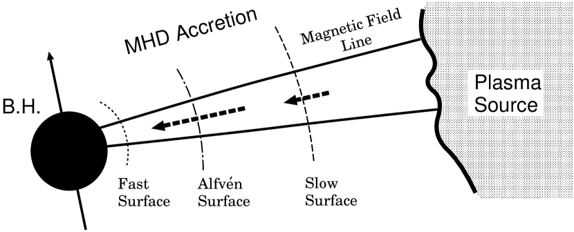
Figure 1: MHD accretion onto a black hole. The flow injected from a plasma source (e.g., the disk surface or the corona) passes through the slow magnetosonic point, the Alfvén point and the fast magnetosonic point, in order, and then goes across the event horizon.

The main purpose of this paper is to examine the thermal effects on an ideal MHD plasma streaming in a black hole magnetosphere (see Fig. 1) by studying the critical conditions at those magnetosonic points. Now, the slow magnetosonic point appears on the MHD flow solutions. The details of critical conditions at the fast and slow magnetosonic points are discussed in § 3. We derive the critical conditions at the fast and slow magnetosonic points, which are denoted in terms of the location of the fast and slow magnetosonic points, the sound velocity at the fast and slow magnetosonic points and the locations of the Alfvén and light surfaces. In § 4, we clarify the thermal effects on the MHD flows, and discuss its dependence on the rotation of the black hole magnetosphere and the divergence of the cross-section of a magnetic flux-tube along the field line. Then, we can find two kinds of trans-fast MHD flow solutions for both inflows and outflows: “hydro-like” MHD flow and “magneto-like” MHD flow. The main difference between the two solutions is the behavior of the magnetization parameter, which is the ratio of the fluid and electromagnetic parts of the total energy of the flow. The hydro-like MHD flow solution is a somewhat hydrodynamical solution and, in the weak magnetic field limit, this trans-fast magnetosonic flow solution becomes a trans-sonic flow solution discussed by Abramowicz (1981) and Lu (1986) in the hydrodynamical case. We also unify hydrodynamic flows with hot MHD flows in a common formalism. The hydro-like MHD flow solution disappears for a magnetically-dominated magnetosphere. On the contrary, the magneto-like MHD flow solution results in the magnetically-dominated flow, although that disappears for hotter plasma cases. In § 5, we summarize our results.

2 Basic Equations and Trans-Alfvénic MHD Flows

We present basic equations of a stationary and axisymmetric ideal MHD flow. The flow streams along a magnetic field line in the black hole magnetosphere, and accretes onto the black hole or blows away to a far distant region. To determine the configuration of magnetic field lines and the velocity of MHD flows streaming along each magnetic field line, we must solve self-consistently what is called the Bernoulli equation along magnetic field lines and the magnetic force-balance equation. These equations are derived from the equation of motion for relativistic MHD plasma

$$T^{\mu\nu}_{;\nu}=\left[(\rho+P)u^{\mu}u^{\nu}-Pg^{\mu\nu}+\frac{1}{4\pi}\left(F^{\mu\delta}F_{\delta}^{\ \nu}+\frac{1}{4}g^{\mu\nu}F^{2}\right)\right]_{;\nu}=0\ ,$$ (1)

the conservation law for particle number $(nu^{\mu})_{;\mu}=0$, the ideal MHD condition $u^{\mu}F_{\mu\nu}=0$ and Maxwell’s equations. Here, $\rho$, $P$ and $n$ are the total energy density, the pressure of the plasma and the proper particle number density. The electromagnetic field tensor $F^{\mu\nu}$ satisfies Maxwell equations and $u^{\mu}$ is the four-velocity of the plasma. The background metric is written by the Boyer-Lindquist coordinates with $c=G=1$,

$$ds^{2} = \left(1-\frac{2mr}{\Sigma}\right)dt^{2}+\frac{4amr\sin^{2}\theta}{\Sigma}dtd\phi$$

$$-\left(r^{2}+a^{2}+\frac{2a^{2}mr\sin^{2}\theta}{\Sigma}\right)\sin^{2}\theta d\phi^{2}-\frac{\Sigma}{\Delta}dr^{2}-\Sigma d\theta^{2}\ ,$$

where $\Delta\equiv r^{2}-2mr+a^{2}$, $\Sigma\equiv r^{2}+a^{2}\cos^{2}\theta$, and $m$ and $a$ denote the mass and angular momentum per unit mass of the black hole, respectively.

The flow with the above assumptions streams along a magnetic field line, which is expressed by a magnetic stream function $\Psi=\Psi(r,\theta)$ with $\Psi=$ constant; $\Psi$ is basically the toroidal component of the vector potential. Stationarity, axisymmetry and ideal MHD condition require the existence of five constants of motion (e.g., Bekenstein & Oron 1978; Camenzind 1986a). These conserved quantities are the total energy $E(\Psi)$, the total angular momentum $L(\Psi)$, the angular velocity of the field line $\Omega_{F}(\Psi)$ and the particle flux through a flux tube $\eta(\Psi)$, which are given by

$$E = \mu u_{t}-\frac{\Omega_{F}}{4\pi\eta}B_{\phi}\ ,$$ (3)

$$L = -\mu u_{\phi}-\frac{1}{4\pi\eta}B_{\phi}\ ,$$ (4)

$$\Omega_{F} = -\frac{F_{tr}}{F_{\phi r}}\ =\ -\frac{F_{t\theta}}{F_{\phi\theta}}\ ,$$ (5)

$$\eta = \frac{nu_{p}}{B_{p}}\ ,$$ (6)

where $B_{\phi}\equiv(\Delta/\Sigma)\sin\theta\;F_{\theta r}$ is the toroidal component of the magnetic field, $B_{p}$ is the poloidal component of the magnetic field seen by a lab-frame observer

$$B_{p}^{2}\equiv-\frac{1}{\rho_{w}^{2}}\left[g^{rr}(\partial_{r}\Psi)^{2}+g^{\theta\theta}(\partial_{\theta}\Psi)^{2}\right]\ ,$$ (7)

and $\rho_{w}^{2}\equiv g_{t\phi}^{2}-g_{tt}g_{\phi\phi}$. The poloidal component $u_{p}$ of the velocity is defined by $u_{p}^{2}\equiv-u_{A}u^{A}$ ($A=r$, $\theta$), where we set $u_{p}>0$ $(u^{r}<0)$ for ingoing flows. For the polytropic equation of state with adiabatic index $\Gamma$, the relativistic specific enthalpy $\mu$ is written as (see Camenzind 1987),

$$\mu=m_{\rm p}\left[1+h_{\rm inj}\left(\frac{u_{p}^{\rm inj}B_{p}}{u_{p}B_{p}^{\rm inj}}\right)^{\Gamma-1}\right]\ ,$$ (8)

where

$$h_{\rm inj}\equiv\frac{\Gamma}{\Gamma-1}\frac{P_{\rm inj}}{n_{\rm inj}m_{\rm p}}\ ,$$ (9)

and $m_{\rm p}$ is the rest mass of the particle. The quantities labeled by “inj” are specified at a point injecting plasma as a plasma source. The boundary conditions should be given by a plasma source model (e.g., the accretion disk/corona model, pair-creation model, and so on). Thus, we require the specification of the additional fifth constant of motion, $h_{\rm inj}$; in a cold limit, we obtain $h_{\rm inj}\to 0$ and $\mu\to m_{\rm p}\,(\equiv\mu_{\rm c})$.

By using the conserved quantities, the equation of motion projected onto the direction of a poloidal magnetic field, which is called the poloidal equation (and is often referred to as the relativistic Bernoulli equation), can be expressed by (e.g., Paper I)

$$(1+u_{p}^{2})=(E/\mu)^{2}\left[(\alpha-2M^{2})f^{2}-k\right]\ ,$$ (10)

where

$$\alpha \equiv g_{tt}+2g_{t\phi}\Omega_{F}+g_{\phi\phi}\Omega_{F}^{2}\ ,$$ (11)

$$k \equiv (g_{\phi\phi}+2g_{t\phi}{\tilde{L}}+g_{tt}{\tilde{L}}^{2})/\rho_{w}^{2}\ ,$$ (12)

$$f \equiv -\ \frac{(g_{t\phi}+g_{\phi\phi}\Omega_{F})+(g_{tt}+g_{t\phi}\Omega_{F}){\tilde{L}}}{\rho_{w}(M^{2}-\alpha)}\ ,$$ (13)

and $\tilde{L}\equiv L/E$. The relativistic Alfvén Mach-number $M$ is defined by

$$M^{2}\equiv\frac{4\pi\mu nu_{p}^{2}}{B_{p}^{2}}=\frac{4\pi\mu\eta u_{p}}{B_{p}}\ .$$ (14)

Note that $\alpha^{-1/2}$ is the “gravitational Lorentz factor” of the plasma rotating with the angular velocity $\Omega_{F}$ in the Kerr geometry, whose definition includes both the effects of the gravitational red-shift and the relativistic bulk motion in the toroidal direction. The locations of the Alfvén points $(r_{\rm A},\theta_{\rm A})$ along a magnetic field line, where $\theta=\theta(r;\Psi)$, are defined by $M^{2}=\alpha$.

The relativistic force-balance equation, which is the equation of motion projected perpendicular to the magnetic surfaces, was derived by Nitta, Takahashi, & Tomimatsu (1991); see also Beskin (1997). We should solve both the poloidal equation and the force-balance equation, but it is too difficult to solve these equations self-consistently. So, we only discuss the poloidal equation on a given magnetic field line. When the poloidal field geometry $\Psi=\Psi(r,\theta)$ is known and the various conserved quantities are specified at the injection point, the Mach-number (14) used together with equation(8) in the poloidal equation (10) determines a complicated equation for $u_{p}$ as a function of $r$. It seems that, to obtain the poloidal velocity, we must solve a polynomial of degree $4N+2$ in $z=u_{p}^{1/N}$ for the polytropic index $N=1/(\Gamma-1)$ (Camenzind 1987). To study the behavior of accretion and wind/jet solutions, however, we can reduce the poloidal equation to

$$E^{2}=\frac{\mu^{2}(1+u_{p}^{2})(\alpha-M^{2})^{2}}{{\cal R}},$$ (15)

where ${\cal R}\equiv{\tilde{e}}^{2}\alpha-2{\tilde{e}}^{2}M^{2}-kM^{4}$ and ${\tilde{e}}\equiv 1-\Omega_{F}\tilde{L}$, and we can plot a contour map of $(E/\mu_{\rm c})^{2}$ easily on the $r$-$u_{p}$ plane under the given flow parameters $\Omega_{F}$, $\tilde{L}$, $\eta$ and $h_{\rm inj}$. The regions with ${\cal R}<0$, where $E^{2}<0$ and no physical flow solution exists, give the forbidden regions of the flow solution on the $r$-$u_{p}$ plane; the shape of the forbidden regions are classified by $\Omega_{F}$ and $\tilde{L}$ (see Paper I for the details of the forbidden regions). Note that, near the inner and outer light surfaces ($r=r_{\rm L}^{in}$ and $r=r_{\rm L}^{out}$) defined by $\alpha=0$, the toroidal velocity of the plasma approaches the light speed. However, if the ideal MHD condition breaks there because of the inertia effects, the plasma would enter the forbidden region $R<0$ by crossing the magnetic field lines; the non-ideal MHD flows are no longer forbidden in the $R<0$ regions. The breakdown of ideal MHD for accretion near the inner light surface is discussed in the last section.

At the Alfvén point (A), where $r=r_{\rm A}$ and $M^{2}=\alpha$, it seems that the function $f$ diverges. However, to obtain a physical accretion solution passing through this point smoothly, we must require the following condition

$${\tilde{L}}=\frac{(-g_{\phi\phi})_{\rm A}(\Omega_{F}-\omega_{\rm A})}{(g_{tt}+g_{t\phi}\Omega_{F})_{\rm A}}\ ,$$ (16)

where $\omega\equiv-g_{t\phi}/g_{\phi\phi}$ is the angular velocity of the zero angular momentum observer with respect to distant observers and the subscript “A” means the quantities at the Alfvén point. Thus, the ratio of the total angular momentum to the total energy of the flow is determined by the location of the Alfvén point and $\Omega_{F}$. When $0<\Omega_{F}<\omega_{\rm H}$ (classified as “type II” in Paper I), where $\omega_{\rm H}$ is the angular velocity of the black hole, one Alfvén point Aⁱⁿ or A^out appears in the $r$-$u_{p}$ plane. When $\omega_{\rm H}<\Omega_{F}<\Omega_{\rm max}$ (“type I”) or $\Omega_{\rm min}<\Omega_{F}<0$ (“type III”), two Alfvén points Aⁱⁿ and A^in/out appear, where $\Omega_{\rm min}$ and $\Omega_{\rm max}$ are the minimum and maximum angular frequency for the light surfaces to exist in the magnetosphere. If two Alfvén points appear in the $r$-$u_{p}$ plane, the physical flow solution passes through one of them. The Alfvén point labeled by “in” or “out” corresponds to inside or outside the separation point $r=r_{\rm sp}$ (SP) which is defined by $\alpha^{\prime}=0$. At $r=r_{\rm sp}$, the gravitational force and the centrifugal force on plasma are balanced if the poloidal velocity of the plasma is zero, hence the term separation point. Although the Alfvén point is classified into three types, one can interpret that the MHD flow of type I, II or III accretes onto a slow-rotating, rapid-rotating or counter-rotating black hole, respectively, when the value of $\Omega_{F}$ is specified.

From equations (10) and (16), we can express the total energy $E$ and the total angular momentum $L$ as functions of the Alfvén radius and the injection point as follows:

$$E = \frac{(g_{tt}+g_{t\phi}\Omega_{F})_{\rm A}}{\alpha_{\rm A}}{\cal E}\ ,$$ (17)

$$L = \frac{(-g_{\phi\phi})_{\rm A}(\Omega_{F}-\omega_{\rm A})}{\alpha_{\rm A}}{\cal E}\ ,$$ (18)

where ${\cal E}\equiv E-\Omega_{F}L>0$ can be specified at the plasma injection point and the Alfvén point. The condition of a negative energy MHD accretion flow, $(g_{tt}+g_{t\phi}\Omega_{F})_{\rm A}<0$, is unchanged from the cold limit case (see Paper I). Thermal effects on the hot plasma flow are only included in ${\cal E}$, and modify the amplitude of the ingoing energy and angular momentum.

3 Critical Conditions at Magnetosonic Points

For a physical solution for accretion onto a black hole, we also require that the critical conditions at both fast and slow magnetosonic points must be satisfied. In this section, we discuss restrictions on the remaining field-aligned parameters; we see that the locations of the fast and slow magnetosonic points give the total energy and the particle number flux along the magnetic field lines.

The differential form of the poloidal equation (10) is written by (see Paper I)

$$(\ln u_{p})^{\prime}=\frac{{\cal N}}{{\cal D}}\ ,$$ (19)

where

$${\cal N} = \left(\frac{E}{\mu}\right)^{2}\left\{\left[{\cal R}(M^{2}-\alpha)C_{\rm sw}^{2}+M^{4}{\cal A}^{2}\right](\ln B_{p})^{\prime}+\frac{1}{2}(1+C_{\rm sw}^{2})\left[M^{4}(M^{2}-\alpha)k^{\prime}-{\cal Q}\alpha^{\prime}\right]\right\}\ ,$$ (20)

$${\cal D} = (M^{2}-\alpha)^{2}\left[(C_{\rm sw}^{2}-u_{p}^{2})(M^{2}-\alpha)+(1+u_{p}^{2})M^{4}{\cal A}^{2}{\cal R}^{-1}\right]\$$ (21)

with ${\cal A}^{2}\equiv{\tilde{e}}^{2}+\alpha k=f^{2}(M^{2}-\alpha)^{2}$ and ${\cal Q}\equiv\alpha{\tilde{e}}^{2}-3{\tilde{e}}^{2}M^{2}-2kM^{4}$. The prime $(\cdots)^{\prime}$ denotes $[(\partial_{\theta}\Psi)\partial_{r}-(\partial_{r}\Psi)\partial_{\theta}]/(\sqrt{-g}B_{p})$ which is a derivative along a stream line. The relativistic sound velocity $a_{\rm sw}$ is given by

$$a_{\rm sw}^{2}\equiv\left(\frac{\partial\ln\mu}{\partial\ln n}\right)_{\rm ad}=(\Gamma-1)\frac{\mu-m_{\rm p}}{\mu}\ ,$$ (22)

and the sound four-velocity is given by $C_{\rm sw}^{2}=a_{\rm sw}^{2}/(1-a_{\rm sw}^{2})$.

The denominator (21) can be reduced to the form

$${\cal D}\propto\left(u_{p}^{2}-u_{\rm AW}^{2}\right)^{2}\left(u_{p}^{2}-u_{\rm FM}^{2}\right)\left(u_{p}^{2}-u_{\rm SM}^{2}\right)\ ,$$ (23)

where the relativistic Alfvén wave speed $u_{\rm AW}$, the fast magnetosonic wave speed $u_{\rm FM}$ and the slow magnetosonic wave speed $u_{\rm SM}$ are defined by

$$u_{\rm AW}^{2}(r;\Psi) \equiv \frac{B_{p}^{2}}{4\pi\mu n}\alpha\ ,$$ (24)

$$u_{\rm FM}^{2}(r;\Psi) \equiv \frac{1}{2}\left({\cal Z}+\sqrt{{\cal Z}^{2}-4C_{\rm sw}^{2}u_{\rm AW}^{2}}\right)\ ,$$ (25)

$$u_{\rm SM}^{2}(r;\Psi) \equiv \frac{1}{2}\left({\cal Z}-\sqrt{{\cal Z}^{2}-4C_{\rm sw}^{2}u_{\rm AW}^{2}}\right)\ ,$$ (26)

with

$${\cal Z} \equiv u_{\rm AW}^{2}+\frac{B_{\phi}^{2}}{4\pi\mu n\rho_{w}^{2}}+C_{\rm sw}^{2}\ ,$$ (27)

$$B_{\phi} = -4\pi\eta E\rho_{w}f\ .$$ (28)

When $u_{p}^{2}=u_{\rm AW}^{2}$, $u_{p}^{2}=u_{\rm FM}^{2}$ or $u_{p}^{2}=u_{\rm SM}^{2}$, the denominator becomes zero. Therefore, at these singular points, we must require ${\cal N}=0$ to obtain physical accretion solutions which pass through these points smoothly. The location of $u_{p}^{2}=u_{\rm A}^{2}$ [$\equiv u_{\rm AW}^{2}(r_{\rm A};\Psi)$] is the Alfvén point discussed in the previous section. Similarly, the locations of $u_{p}^{2}=u_{\rm F}^{2}$ [$\equiv u_{\rm FM}^{2}(r_{\rm F};\Psi)$] and $u_{p}^{2}=u_{\rm S}^{2}$ [$\equiv u_{\rm SM}^{2}(r_{\rm S};\Psi)$] correspond to the fast magnetosonic point $r=r_{\rm F}$ and the slow magnetosonic point $r=r_{\rm S}$, respectively. We should mention that, to calculate the Alfvén velocity, we need to solve a polynomial of high degree, while in the cold limit it is simply obtained as $u_{\rm A}^{\rm cold}=(\alpha B_{p})_{\rm A}/(4\pi\mu_{\rm c}\eta)$; the Alfvén velocity of a hot MHD flow is always smaller than $u_{\rm A}^{\rm cold}$.

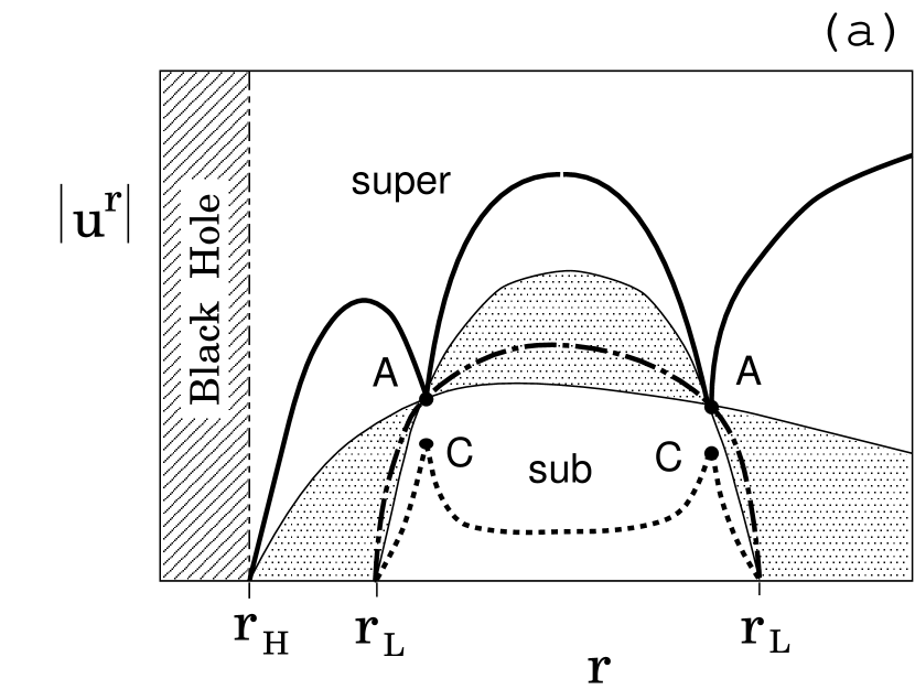
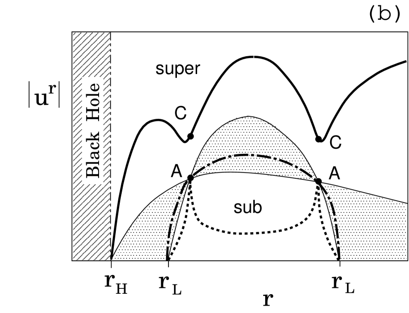
Figure 2: Schematic pictures of ${\cal D}(r,u^{r})=0$ curves for (a) strong magnetic field $(C_{\rm sw}^{2})_{\rm A}<u_{\rm A}^{2}$ and (b) weak magnetic field $(C_{\rm sw}^{2})_{\rm A}>u_{\rm A}^{2}$. The thick-solid-curves correspond to the $u_{p}^{2}=u_{\rm FM}^{2}$ curves; the thick-dash-dot-curves correspond to the $u_{p}^{2}=u_{\rm AW}^{2}$ curves; and the thick-dotted-curves correspond to the $u_{p}^{2}=u_{\rm SM}^{2}$ curves. The shaded regions are forbidden regions of flows (type IA or IIIA), and separate the super-Alfvénic region labeled by “super” from the sub-Alfvénic region labeled by “sub”. The hatched region is inside the black hole.

Figure 2 shows schematic pictures of the ${\cal D}=0$ curves in the $r$-$u^{r}$ plane. [The definition of the poloidal velocity $u_{p}$ includes the gravitational-redshift factor, so that $u_{p}$ diverges at the event horizon for a physical accretion solution. Hereafter we use the $r$-$u^{r}$ plane when we discuss the behavior of accretion solutions; under a given magnetic field with $\Psi(r,\theta)=$ constant, we can also calculate $\theta=\theta(r;\Psi)$ and $u^{\theta}=u^{\theta}(r;\Psi)$. ] Corresponding to the two modes of magnetosonic wave speeds and the Alfvén wave speed, we see three branches of ${\cal D}=0$ curves, which correspond to $u_{p}^{2}=u_{\rm FM}^{2}$, $u_{p}^{2}=u_{\rm SM}^{2}$ and $u_{p}^{2}=u_{\rm AW}^{2}$ curves. The $u_{p}^{2}=u_{\rm AW}^{2}$ curve is always located inside the forbidden region (the shaded regions) except for the Alfvén point, so these forbidden regions separate the $r$-$u^{r}$ plane into one or two super-Alfvénic region(s) and one sub-Alfvénic region. If there is no area of $k(r;\tilde{L})>0$, we see one super-Alfvénic and one sub-Alfvénic regions with forbidden regions classified as “type A” in Paper I. The total angular momentum has a value of $\tilde{L}_{-}<\tilde{L}<\tilde{L}_{+}$, where $\tilde{L}=\tilde{L}_{+}(>0)$ and $\tilde{L}=\tilde{L}_{-}(<0)$ are the minimum and maximum values of the function $\tilde{L}=\tilde{L}(r_{\rm A};\Omega_{F})$. On the other hand, if an area with $k>0$ exists between two light surfaces, we see two super-Alfvénic regions separated by “type B” forbidden regions, and obtain larger total angular momentum MHD flows ($\tilde{L}>\tilde{L}_{+}$ or $|\tilde{L}|>|\tilde{L}_{-}|$). Thus, we can classify the forbidden regions by $\Omega_{F}$ and $\tilde{L}$ as type I, II or III and type A or B, independently; hereafter, we will denote the type of forbidden regions as, for example, type IA.

The $u_{p}^{2}=u_{\rm FM}^{2}$ and $u_{p}^{2}=u_{\rm SM}^{2}$ curves are located in the super-Alfvénic region and the sub-Alfvénic region, respectively. Figure 2a shows a case for strong magnetic fields satisfying $(C_{\rm sw}^{2})_{\rm A}<u_{\rm A}^{2}$, and Figure 2b shows a case for weak magnetic fields satisfying $(C_{\rm sw}^{2})_{\rm A}>u_{\rm A}^{2}$. In Figure 2a the $u_{p}^{2}=u_{\rm FM}^{2}$ curve connects to the Alfvén point marked by “A” ($r=r_{\rm A},u_{p}^{2}=u_{\rm A}^{2}$), while in Figure 2b the $u_{p}^{2}=u_{\rm SM}^{2}$ curve connects to the Alfvén point. At the Alfvén radius $r=r_{\rm A}$ the value of the function $f=f(u_{p};r_{\rm A})$ is zero except at the Alfvén point A. Then, $u_{p}^{2}=C_{\rm sw}^{2}$ is one of the solutions of ${\cal D}(u_{p};r_{\rm A})=0$ (marked by “C” in Fig. 2). A similar situation at the (outer) Alfvén point can be seen in the Newtonian case (see Heyvaerts & Norman (1989)).

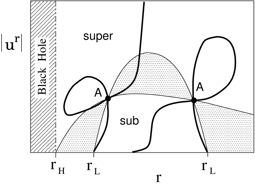
Figure 3: A schematic picture of ${\cal N}(r,u^{r})=0$ curves. The shaded regions are forbidden regions (type IA or IIIA).

We also plot a typical curve with ${\cal N}=0$ in Figure 3. Crossing of the ${\cal D}=0$ curves and ${\cal N}=0$ curves in the super- or sub-Alfvénic region means the fast or slow magnetosonic point, respectively. In the cold limit, between the Alfvén point and the event horizon in the super-Alfvénic region, crossing of the ${\cal N}=0$ curve and ${\cal D}=0$ curve always exists regardless of the $\eta$ value (Paper I). However, in the case of $(C_{\rm sw}^{2})_{\rm A}>u_{\rm A}^{2}$, we cannot find any reason for crossing of these lines. In fact, we find a restriction on the hot trans-fast MHD accretion by the thermal effects. In this case, the condition ${\cal N}={\cal D}=0$ is not achieved between the inner Alfvén radius and the event horizon; that is, no physical trans-fast MHD accretion solution exists. When the thermal effects dominate over the magnetic effects, we can find that the crossing of these lines is only available for smaller $|\eta|$, while for larger $|\eta|$ it becomes impossible to generate a physical trans-fast MHD accretion solution (see below). In the cold limit, because the slow magnetosonic wave speed is zero, the X-type slow magnetosonic point is located just on the $r$-axis ($u^{r}=0$ line), which is just the separation point. When thermal effects are effective, we can see X-type slow magnetosonic points with a sub-slow magnetosonic region in the sub-Alfvénic region of the $r$-$u^{r}$ plane.

Now, we will discuss the condition for crossings of the ${\cal N}(r,u_{p})=0$ and ${\cal D}(r,u_{p})=0$ curves. We use the indices “F” and “S” to denote the quantities evaluated at the fast and slow magnetosonic points, respectively, and use the index “cr” to unite the quantities at these magnetosonic points. In the following equations, to discuss MHD flows passing through the fast or slow magnetosonic point, we can replace the subscript “cr” by “F” or “S”. From the condition ${\cal D}=0$ at the fast and slow magnetosonic points, the poloidal velocity at these critical points $u_{\rm cr}^{2}\equiv u_{p}^{2}(r_{\rm cr};\Psi)$ is written as

$$u_{\rm cr}^{2}=\left[\frac{{\cal R}C_{\rm sw}^{2}(M^{2}-\alpha)+M^{4}{\cal A}^{2}}{{\cal R}(M^{2}-\alpha)-M^{4}{\cal A}^{2}}\right]_{\rm cr}\ ,$$ (29)

and by use of the definition of Mach-number (14), the particle flux through a flux tube $\eta$ is determined by

$$\eta=\left(\frac{B_{p}}{4\pi\mu}\right)_{\rm cr}\frac{M^{2}_{\rm cr}}{u_{\rm cr}}\ ,$$ (30)

where the critical Mach-number $M_{\rm cr}^{2}\equiv M^{2}(r_{\rm cr};\Psi)$ is obtained as a solution of ${\cal N}=0$, which is a cubic equation in $M^{2}$. Thus, we can express $\eta$ as a function of $r_{\rm cr}$ with given parameters $\Omega_{F}$, $\tilde{L}$, $(a_{\rm sw}^{2})_{\rm cr}$ and $\Psi$. The total energy of the trans-fast (or trans-slow) MHD flow is also evaluated at the fast (or slow) magnetosonic point $r_{\rm F}$ (or $r_{\rm S}$) by using the poloidal equation (15). Here, we would like to emphasize that $(a_{\rm sw}^{2})_{\rm cr}$ is introduced as a parameter for the thermal effects on the trans-fast MHD flows instead of $(a_{\rm sw}^{2})_{\rm inj}$ (or $h_{\rm inj}$). The acceptable ranges for $(a_{\rm sw}^{2})_{\rm S}$ and $(a_{\rm sw}^{2})_{\rm F}$ are restricted by the critical condition (30), which is to be realized as trans-slow and trans-fast MHD accretion, respectively. Thus, all boundary conditions can be replaced by the Alfvén and magnetosonic conditions. The behavior of $\eta=\eta[r_{\rm cr};\Omega_{F},\tilde{L},(a_{\rm sw}^{2})_{\rm cr};a,\Psi]$ will be discussed in the next section.

4 Thermal Effects on Trans-Fast MHD Flows

Let us discuss a trans-fast MHD flow in a black hole magnetosphere. We consider magnetic flux-tubes given by $\partial_{r}\Psi=0$ and $\partial_{\theta}\Psi=C\,r^{-\delta}\,\sin\theta$; that is, the poloidal magnetic field is denoted as $B_{p}(r;\Psi)=(C/\sqrt{\Delta\Sigma})\,r^{-\delta}$, where $\delta=\delta(\Psi)$ and $C=C(\Psi)$; $\delta$ is related to the divergence of a magnetic flux tube. For example, $\delta=0$ with $C(\Psi)=$ constant means the split monopole magnetic field (Blandford & Znajek, 1977). Hereafter, we consider a situation where the plasma streams close to the equatorial plane. We expect that the qualitative picture is not drastically changed when we leave the equatorial plane and when we consider more complicated field geometries.

4.1 Restrictions on Trans-Fast MHD Flow Solutions

We introduce a new parameter $x_{\rm A}$ to specify the Alfvén radius by $x_{\rm A}\equiv(r_{\rm sp}-r_{\rm A})/(r_{\rm sp}-r_{\rm L}^{in})$, where $0<x_{\rm A}<1$. Though, for a given $x_{\rm A}$, we obtain a value of $\tilde{L}$, we may find another value for $x_{\rm A}$ giving the same $\tilde{L}$ value in the cases with types I and III; that is, we may see two Alfvén points inside the separation point. Further, we introduce $\hat{\eta}\equiv\mu_{\rm c}|\eta/C|$ and $\zeta_{\rm cr}\equiv(a_{\rm sw}^{2})_{\rm cr}$.

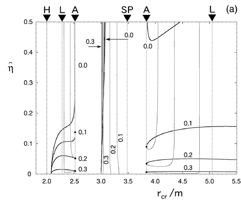
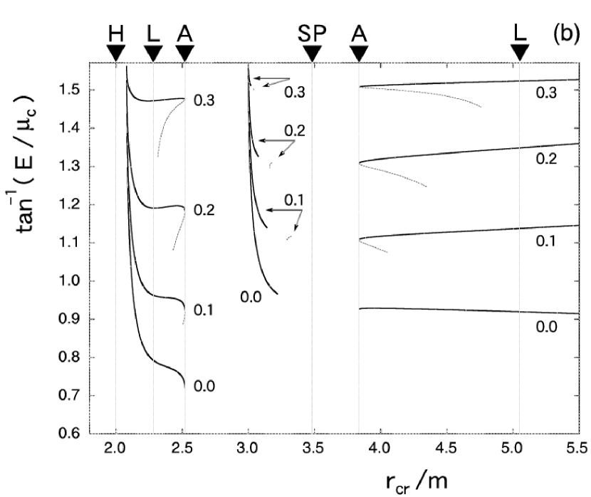
Figure 4: (a) Relations between $r_{\rm cr}$ and $\hat{\eta}$ and (b) relations between $E/\mu_{\rm c}$ and $r_{\rm cr}$ for a radial flow with $\delta=0$ in a Schwarzschild black hole magnetosphere with several $\zeta_{\rm cr}$ values (0.00, 0.10, 0.20, 0.30). The angular velocity of the magnetic field is $\Omega_{F}=0.8\Omega_{\rm max}$, where $m\Omega_{\rm max}=0.192$. The location of the Alfvén point is specified by $x_{\rm A}=0.8$, which corresponds to $\Omega_{F}\tilde{L}=0.7287$. The solid-curves indicate $\hat{\eta}=\hat{\eta}(r_{\rm F})$ with $r_{\rm cr}=r_{\rm F}$. The dashed-curves indicate $\hat{\eta}=\hat{\eta}(r_{\rm S})$ with $r_{\rm cr}=r_{\rm S}$. The shape of forbidden regions corresponds to type IA.

Figures 4a, 5–8 show relations between $\hat{\eta}$ and $r_{\rm cr}$ for various $\zeta_{\rm cr}$ values under given parameters $\Omega_{F}$, $\tilde{L}$, $\delta$ and the spin parameter $a$; The locations of $r_{\rm cr}=r_{\rm H}$, $r_{\rm cr}=r_{\rm L}^{in/out}$, $r_{\rm cr}=r_{\rm A}^{in/out}$ and $r_{\rm cr}=r_{\rm sp}$ are marked by H, L, A and SP, respectively. Here, we will discuss the magnetosonic points located inside the outer light surface, because for accretion the fast magnetosonic point should be located inside the outer Alfvén point and the slow magnetosonic point should be located between the inner Alfvén point and the outer light surface.

4.1.1 General Properties

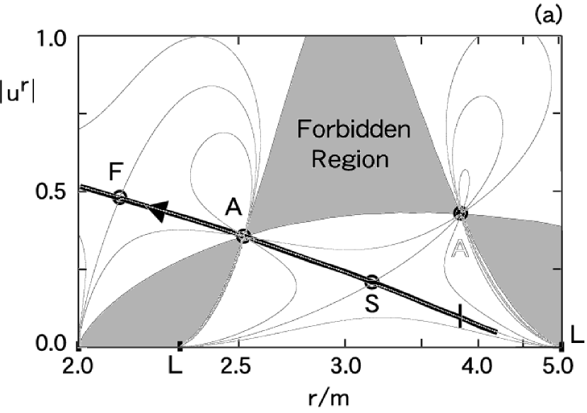
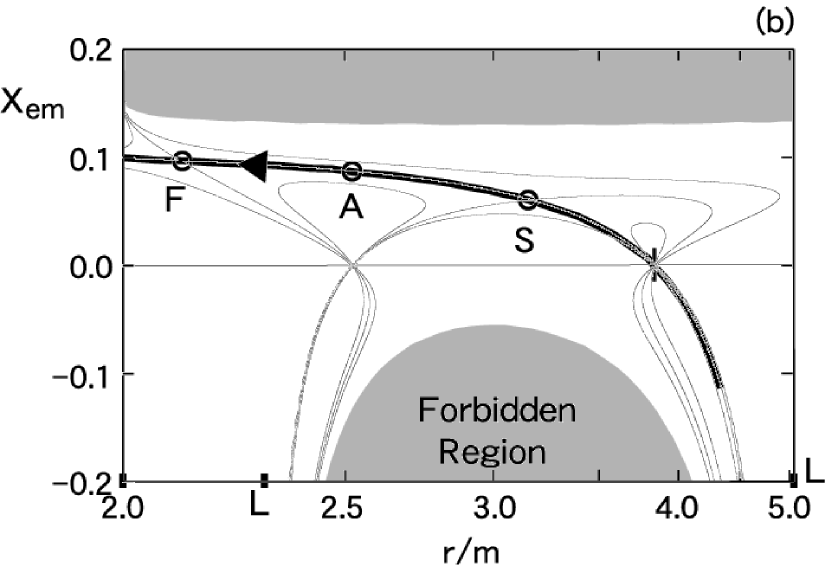
Figure 10: An example of the trans-fast MHD accretion solution (thick curves); (a) radial 4-velocity and (b) the ratio of the electromagnetic energy to the total energy. This solution passes through the inner Alfvén point and the inner fast magnetosonic point (S $\to$ A $\to$ F $\to$ H), where $a=0.0$, $\Omega_{F}=0.8\Omega_{\rm max}$, $\delta=0.0$, $\Gamma=4/3$ and $\zeta_{\rm F}=0.2$. The location of the Alfvén point is specified by $x_{\rm A}=0.8$, which corresponds to $\Omega_{F}\tilde{L}=0.7287$. The location of the fast magnetosonic point is $r_{\rm F}=2.10935m$, which gives $E_{\rm F}/\mu_{\rm c}=3.6643$ and $\hat{\eta}=0.0337$. The requirement that $\hat{\eta}<\hat{\eta}_{\rm max}$ is satisfied.

In the cold limit, there are three branches of $\hat{\eta}=\hat{\eta}(r_{\rm F})$ (solid curves with $\zeta_{\rm cr}=0.0$), while there is no $\hat{\eta}=\hat{\eta}(r_{\rm S})$ curve. For hot MHD flows with $\zeta_{\rm cr}=0.1,0.2$ and $0.3$, however, both $\hat{\eta}=\hat{\eta}(r_{\rm F})$ and $\hat{\eta}=\hat{\eta}(r_{\rm S})$ curves (dashed curves) exist. When we try to plot a contour map of $(E/\mu_{\rm c})^{2}$ on the $r$-$u^{r}$ plane as an accretion solution (see, e.g., Fig. 10a), from the $\hat{\eta}$ vs. $r_{\rm cr}$ diagram we can find the acceptable locations of the fast/slow magnetosonic points, which are shown as the crossings of a $\hat{\eta}=$ constant line and $\hat{\eta}=\hat{\eta}(r_{\rm cr};\zeta_{\rm cr})$ curves. Hereafter, the magnetosonic points located inside the inner Alfvén point are labeled as “in”, the middle magnetosonic points located between two Alfvén points are labeled as “mid” and the magnetosonic points located outside the outer Alfvén point are labeled as “out”. In Figures 4a, 5–8, the location of $\hat{\eta}(r_{\rm cr};\zeta_{\rm cr})=0$ exists between $r_{\rm F}=r_{\rm H}$ and $r_{\rm F}=r_{\rm A}^{in}$; The location does not depend on the $\zeta_{\rm F}$ values. For hot MHD flows we can see the cases where $\hat{\eta}=\hat{\eta}(r_{\rm F})$ curves and $\hat{\eta}=\hat{\eta}(r_{\rm S})$ curves are connected at $r_{\rm cr}=r_{\rm A}$ (the locations marked by “$\bullet$”). For the fast magnetosonic point located just inside (or outside) the Alfvén point, from ${\cal N}=0$ we have

$$M_{\rm F}^{2}=\alpha_{\rm A}+{\cal Y}_{\rm A}|{\cal A}|^{1/2}+O({\cal A})$$ (31)

where

$${\cal Y}\equiv\frac{{\cal A}}{|{\cal A}|}\frac{\{6{\tilde{e}}^{2}[a_{\rm sw}^{2}(\ln B_{p})^{\prime}]^{2}-2{\tilde{e}}^{2}a_{\rm sw}^{2}(\ln B_{p})^{\prime}{\cal A}^{\prime}+k\alpha^{\prime}{\cal A}^{\prime}\}^{1/2}}{-ka_{\rm sw}^{2}(\ln B_{p})^{\prime}+(k/2)^{\prime}}\ .$$ (32)

In the $r_{\rm F}\to r_{\rm A}$ (${\cal A}\to 0$) limit, from equation (30), the value of $\eta$ is given by

$$\hat{\eta}_{\ast} \equiv \lim_{r_{\rm F}\to r_{\rm A}}\hat{\eta}$$ (33)

$$= \left[\frac{(B_{p}/C)\alpha}{4\pi(\mu/\mu_{\rm c})}\right]_{\rm A}\left[\frac{k\{6{\tilde{e}}^{2}[a_{\rm sw}^{2}(\ln B_{p})^{\prime}]^{2}-2{\tilde{e}}^{2}a_{\rm sw}^{2}(\ln B_{p})^{\prime}{\cal A}^{\prime}+k\alpha^{\prime}{\cal A}^{\prime}\}}{a_{\rm sw}^{2}\{[2ka_{\rm sw}^{2}(\ln B_{p})^{\prime}-k^{\prime}]\alpha k{\cal A}^{\prime}+3{\tilde{e}}^{2}a_{\rm sw}^{2}(\ln B_{p})^{\prime}k^{\prime}\}}-1\right]^{1/2}_{\rm A}\ .$$

Then, $\hat{\eta}$ for hot MHD accretion passing through the inner-fast magnetosonic point has an upper-limit. Thus, the thermal effect restricts the acceptable $\hat{\eta}$ values, while in the cold limit the range is given by $0<\hat{\eta}<\infty$. Figures 4a, 5–8 also show that the $\hat{\eta}=\hat{\eta}(r_{\rm F}^{\rm in})$ and $\hat{\eta}=\hat{\eta}(r_{\rm F}^{\rm out})$ curves shrink down vertically with increasing $\zeta_{\rm F}$. When $\zeta_{\rm F}\geq 0.3$, the magnetic effect on the plasma can still remain efficient for the flows passing through $r_{\rm F}^{\rm in}$ or $r_{\rm F}^{\rm out}$ which gives a trans-fast MHD flow with $\hat{\eta}\ll 1$. On the other hand, the $\hat{\eta}=\hat{\eta}(r_{\rm S}^{\rm in})$ and $\hat{\eta}=\hat{\eta}(r_{\rm S}^{\rm out})$ curves become almost vertical when $\hat{\eta}$ is at least several times as large as $\hat{\eta}_{\ast}$; that is, the location of the slow magnetosonic point is almost independent of $\hat{\eta}$, and the curves shift toward the inner and outer light surfaces with increasing $\zeta_{\rm S}$, respectively. We should note that an ideal MHD accretion flow after passing through the inner-slow magnetosonic point is impossible, because no Alfvén point is located inside this slow magnetosonic point; an outflow may be possible after passing through this slow magnetosonic point, the inner Alfvén point and the middle fast magnetosonic point, in this order.

In contrast to the inner-magnetosonic points, a trans-fast MHD flow passing through the middle-fast magnetosonic point is always available for any $\hat{\eta}$ values. We see that in Figure 4a the location of the middle-fast magnetosonic point is insensitive to both $\hat{\eta}$ and $\zeta_{\rm F}$; and the location of the middle-slow magnetosonic point is insensitive to only $\hat{\eta}$, while it shifts inward with increasing $\zeta_{\rm S}$. We can also see branches for $\hat{\eta}=\hat{\eta}(r_{\rm F}^{\rm out})$ for the fast magnetosonic point located outside the outer Alfvén point. An outgoing flow from the black hole magnetosphere should pass through the outer-fast or middle-fast magnetosonic point after passing through the outer or inner Alfvén point. In this paper, however, we will focus our attention to trans-fast MHD accretion onto a black hole, and omit discussions of the outgoing flows from the magnetosphere.

Figure 4b shows the total energy $E/\mu_{\rm c}$ of the trans-magnetosonic flows as a function of $r_{\rm cr}$. For a fast magnetosonic point giving a smaller $\hat{\eta}$ value, the energy becomes larger. This means that the larger energy is shared by smaller numbers of particles. Corresponding to the “maximum” $\hat{\eta}$ value for $\hat{\eta}=\hat{\eta}(r_{\rm F}^{\rm in})$, a “minimum” value of $E/\mu_{\rm c}$ exists for the $E=E(r_{\rm F}^{\rm in/out})$ curve. For a hotter flow which includes more thermal energy, this minimum value becomes larger than the cooler one. A trans-slow MHD flow passing through the inner-slow or outer-slow magnetosonic point has also a lower limit for the total energy. Furthermore, for the middle-slow magnetosonic point, the acceptable value of $E/\mu_{\rm c}$ is restricted within a very narrow range, while it seems that there is no restriction on $\hat{\eta}$.

4.1.2 Rotational Effects of the Magnetic Field Line

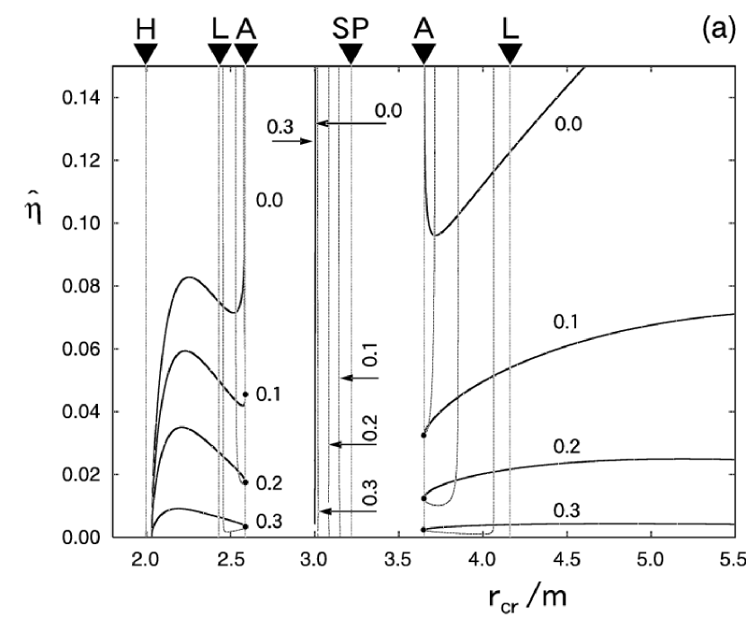
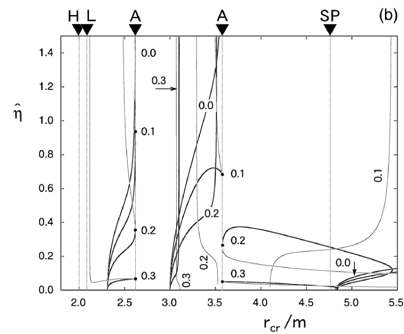
Figure 5: Relations between $\hat{\eta}$ and $r_{\rm cr}$ for a radial flow with $\delta=0$ in a Schwarzschild black hole magnetosphere with several $\zeta_{\rm cr}$ values (0.00, 0.10, 0.20, 0.30). The angular velocities of the magnetic field are (a) $\Omega_{F}=0.9\Omega_{\rm max}$ and (b) $\Omega_{F}=0.5\Omega_{\rm max}$. The location of the Alfvén point is specified by $x_{\rm A}=0.8$, which corresponds to (a) $\Omega_{F}\tilde{L}=0.8841$ and (b) $\Omega_{F}\tilde{L}=0.2687$. The solid-curves indicate $\hat{\eta}=\hat{\eta}(r_{\rm F})$, and the dashed-curves indicate $\hat{\eta}=\hat{\eta}(r_{\rm S})$. The shape of the forbidden regions corresponds to type IA.

From Figures 5 and 4a, we can see the $\Omega_{F}$ dependence of the locations of magnetosonic points. Comparing Figure 5a ($\Omega_{F}=0.9\Omega_{\rm max}$) with Figure 4a ($\Omega_{F}=0.8\Omega_{\rm max}$), the location of the inner light surface moves outward and the locations of the separation point and the outer light surface move inward with increasing $\Omega_{F}$. In both cases, the separation point is located between two Alfvén points. For cooler accretion of $\zeta_{\rm F}\leq 0.1$, three fast magnetosonic points may be possible between the inner Alfvén point and the event horizon (see Fig. 5a). The middle one is an O-type point (unphysical), while the others are X-type critical points (physical). For hotter accretion ($\zeta_{\rm F}\geq 0.1$ at least), however, the X-type fast magnetosonic point located next to the Alfvén point disappears, and it turns to the slow magnetosonic point.

Next, comparing Figure 5b ($\Omega_{F}=0.5\Omega_{\rm max}$) with Figure 4a, the location of the inner light surface moves inward and the locations of the separation point and the outer light surface move outward with decreasing $\Omega_{F}$. Two Alfvén points are located between the inner light surface and the separation point; and then, both the inner and outer Alfvén points, which are labeled by “in” (see § 2), can be related to accretion started near the separation point. Concerning the $\hat{\eta}=\hat{\eta}(r_{\rm F}^{\rm mid})$ branches, which are located between two Alfvén points, a branch of smaller $\zeta_{\rm F}$ (e.g., $\zeta_{\rm F}=0.1$) has a maximum, while a branch of larger $\zeta_{\rm F}$ (e.g., $\zeta_{\rm F}=0.2,0.3$) has no upper limit. We see that for smaller $\zeta_{\rm F}$ the branch for the middle-fast magnetosonic point connects to the outer Alfvén point (see the $\zeta_{\rm F}=0.1$ curve) and for larger $\zeta_{\rm F}$ the branch for the outer-fast magnetosonic point connects to the outer Alfvén point (see $\zeta_{\rm F}=0.2$).

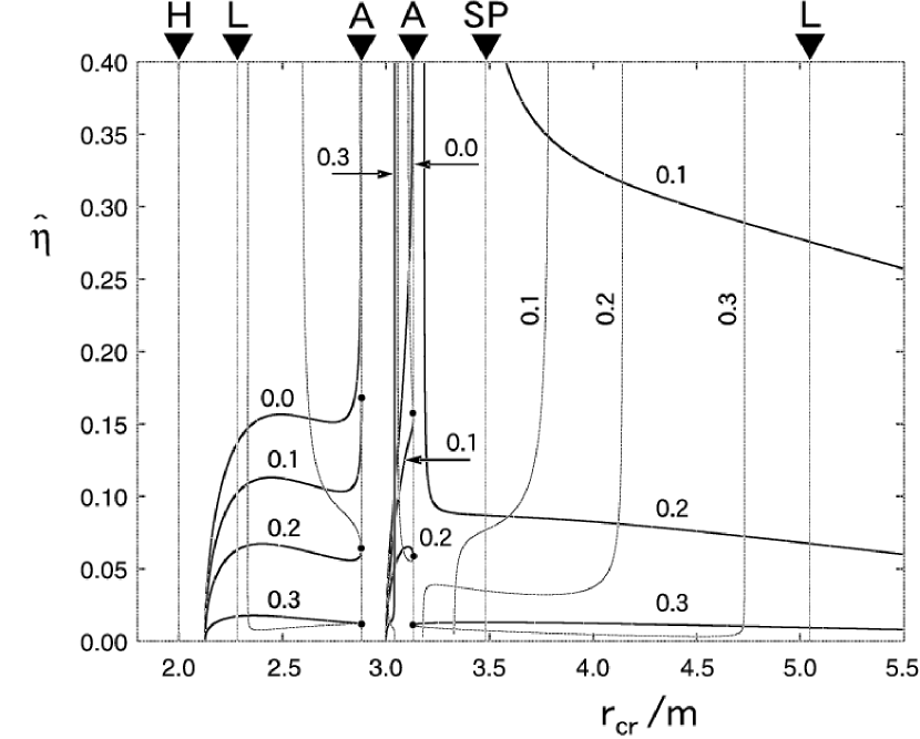
Figure 6: Relations between $\hat{\eta}$ and $r_{\rm cr}$ for a radial flow with $\delta=0$ and several $\zeta_{\rm cr}$ values (0.00, 0.10, 0.20, 0.30) in a Schwarzschild black hole magnetosphere. The angular velocity of the magnetic field is $\Omega_{F}=0.8\Omega_{\rm max}$. The location of the Alfvén point is specified by $x_{\rm A}=0.5$, which corresponds to $\Omega_{F}\tilde{L}=0.6434$. The solid-curves indicate $\hat{\eta}=\hat{\eta}(r_{\rm F})$, and the dashed-curves indicate $\hat{\eta}=\hat{\eta}(r_{\rm S})$. The shape of the forbidden regions corresponds to type IA.

Figure 6 shows $\hat{\eta}$ as a function of $r_{\rm cr}$ with $x_{\rm A}=0.5$. The outer Alfvén point is located inside the separation point. There is an upper limit to the $\hat{\eta}=\hat{\eta}(r_{\rm F}^{\rm mid})$ curve for each of the $\zeta_{\rm F}=0.1$ and $0.2$ cases, while for $\zeta_{\rm F}=0.3$ the middle-fast magnetosonic point always exists for any $\hat{\eta}$ values (no upper limit).

4.1.3 Black Hole’s Spin Effects

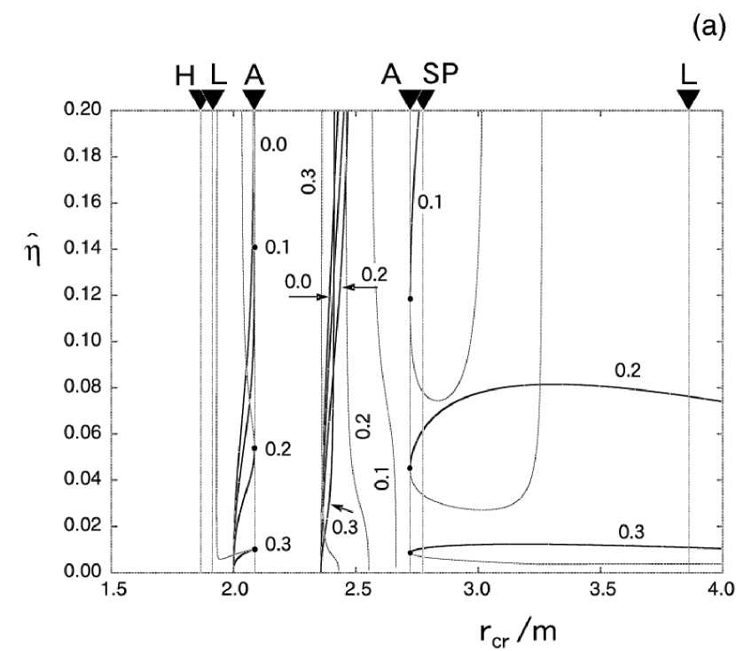
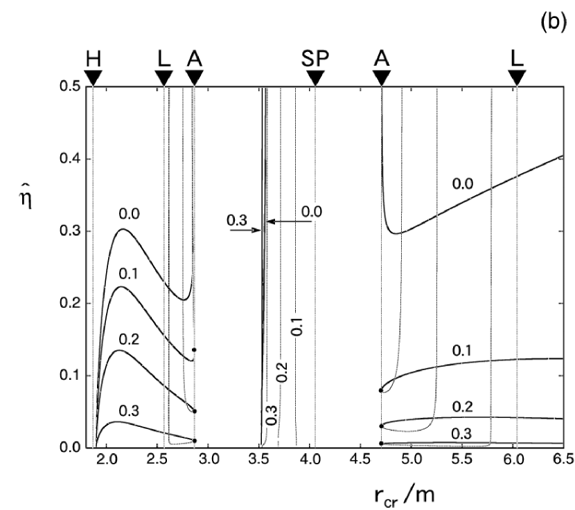
Figure 7: Relations between $\hat{\eta}$ and $r_{\rm cr}$ for a radial flow with $\delta=0$ in a Kerr black hole magnetosphere; (a) $a=0.5m$ and (b) $a=-0.5m$ with several $\zeta_{\rm cr}$ values (0.00, 0.10, 0.20, 0.30). The angular velocity of the magnetic field is $\Omega_{F}=0.8\Omega_{\rm max}$, where (a) $m\Omega_{\rm max}=0.244$ and (b) $m\Omega_{\rm max}=0.163$. The location of the Alfvén point is specified by $x_{\rm A}=0.8$, which corresponds to (a) $\Omega_{F}\tilde{L}=0.6749$ and (b) $\Omega_{F}\tilde{L}=0.7490$. The solid-curves indicate $\hat{\eta}=\hat{\eta}(r_{\rm F})$, and the dashed-curves indicate $\hat{\eta}=\hat{\eta}(r_{\rm S})$. The shape of the forbidden regions corresponds to type IA.

Figures 7a and 7b show the $\hat{\eta}$ vs. $r_{\rm cr}$ relation with $a=0.5m$ (a corotating black hole with the magnetosphere) and $a=-0.5m$ (a counter-rotating black hole), respectively. They can be also compared with Figure 4a, which is the case with $a=0$. In the case with $a=0.5m$, two Alfvén points are located inside the separation point; and the outer Alfvén point is located very close to the separation point. The properties of $\hat{\eta}=\hat{\eta}(r_{\rm cr})$ are similar to the case of Figure 5b. In Figure 7a, it seems that the branches with $\hat{\eta}=\hat{\eta}(r_{\rm F}^{\rm mid})$ have no maximum value, but for cooler flows ($\zeta_{\rm F}\ll 1$) there are branches with $\hat{\eta}=\hat{\eta}(r_{\rm F}^{\rm mid})$ which have a maximum value. In the case of $a=-0.5m$, the separation point is located between two Alfvén points, and the properties of $\hat{\eta}=\hat{\eta}(r_{\rm cr})$ are essentially similar to the cases for Figures 4a and 5a. Comparing Figure 7b with Figure 4, the counter-rotating effect of the black hole generates three (or two) inner-fast magnetosonic points, while the effect of corotation is to suppress such multi-inner-fast magnetosonic points generation (see, e.g., $\hat{\eta}=\hat{\eta}(r_{\rm F}^{\rm in})$ curves with $\zeta_{\rm F}=0.1$ in these figures).

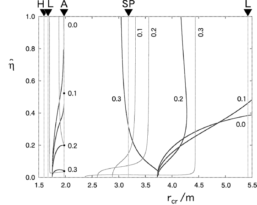
Figure 8: Relations between $\hat{\eta}$ and $r_{\rm cr}$ for a radial flow with $\delta=0$ and several $\zeta_{\rm cr}$ values (0.00, 0.10, 0.20, 0.30) in a Kerr black hole magnetosphere ($a=0.8m$). The angular velocity of the magnetic field is $\Omega_{F}=0.5\Omega_{\rm max}$, where $m\Omega_{\rm max}=0.309$. The location of the Alfvén point is specified by $x_{\rm A}=0.8$, which corresponds to $\Omega_{F}\tilde{L}=-0.0117$. The solid-curves indicate $\hat{\eta}=\hat{\eta}(r_{\rm F})$, and the dashed-curves indicate $\hat{\eta}=\hat{\eta}(r_{\rm S})$. The shape of the forbidden regions corresponds to type IIA.

Figure 8 shows $\hat{\eta}$ as a function of $r_{\rm cr}$ with $a=0.8m$, $x_{\rm A}=0.8$ and $\Omega_{F}=0.5\Omega_{\rm max}$. This is a case of only one Alfvén point and one super-Alfvénic region in the $r$-$u^{r}$ plane (type IIA forbidden region). In the previous examples of type IA forbidden region (i.e., Figs. 4–8), we have seen inner and outer Alfvén points and two regimes of trans-fast MHD accretion solutions. In this case, however, there is one type of solution. The Alfvén point is located inside the separation point, and each branch of $\hat{\eta}=\hat{\eta}(r_{\rm F}^{\rm in})$ has an upper limit for $\hat{\eta}$, except for the cold limit. It seems that for the cooler flows the slow magnetosonic point is located near the separation point, but for the hotter flows the location shifts outward. However, if the hotter flow has a small $\hat{\eta}$, the slow magnetosonic point could be located close to the separation point.

4.1.4 Non-conical Effects of the Magnetic Field Geometry

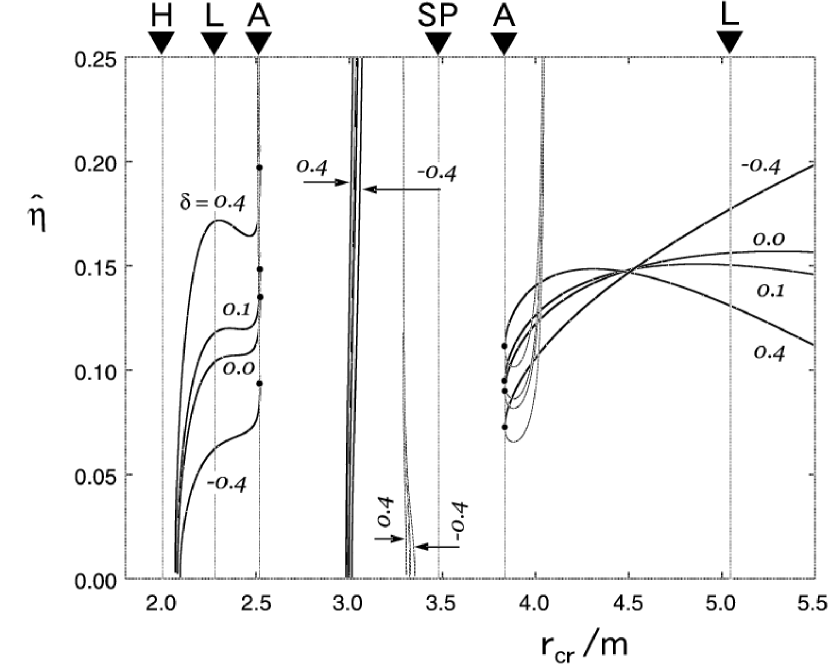
Figure 9: The $\delta$-dependence ($\delta=-0.4,0.0,0.1,0.4$) of the relations between $\hat{\eta}$ and $r_{\rm cr}$, where $a=0.0$, $\zeta_{\rm cr}=0.1$, $\Omega_{F}=0.8\Omega_{\rm max}$ and $x_{\rm A}=0.8$ (see also Fig. 4a). The solid-curves indicate $\hat{\eta}=\hat{\eta}(r_{\rm F})$, and the dashed-curves indicate $\hat{\eta}=\hat{\eta}(r_{\rm S})$. The shape of the forbidden regions corresponds to type IA.

The effects of magnetic field geometry on the critical condition (30) are shown in Figure 9 for a hot MHD flow; The effects of non-conical geometry ($\delta\neq 0$) for cold MHD accretion have been discussed by Takahashi (1994). The maximum $\hat{\eta}$ value increases with increasing $\delta$, for $\hat{\eta}=\hat{\eta}(r_{\rm F}^{\rm in})$ curves. This means that the field geometry converging along an ingoing stream line ($\delta>0$) rather than the radial field is available to make a higher accretion-rate than $\delta<0$ cases. The location of $\hat{\eta}(r_{\rm F})=0$ has a weak dependence on $\delta$. The location of the middle fast magnetosonic point also has a weak dependence on $\delta$, and the slow magnetosonic point remains at a fixed location except for smaller $\hat{\eta}$ cases.

4.2 Two Regimes of Accretion Solutions

Here, we will present accretion solutions. To plot an SAF-solution, we need to determine the five field-aligned constant quantities: $\Omega_{F}$, $L$, $\eta$, $E$, $h_{\rm inj}$. Although these constants should be given as boundary conditions at the plasma source (inj), mathematically we can choose the locations of $r_{\rm F}$, $r_{\rm L}$, $r_{\rm A}$ and the sound velocity $\zeta_{\rm F}$ as free parameters to fix the conserved quantities if one restricts their interest to ideal MHD solutions. First, for the plasma sources to exist in a black hole magnetosphere, we require that $\Omega_{\rm min}<\Omega_{F}<\Omega_{\rm max}$; then, two light surfaces $r=r_{\rm L}^{in}(\Omega_{F};a,\Psi)$ and $r=r_{\rm L}^{out}(\Omega_{F};a,\Psi)$ are determined. Second, from equation (16), $\tilde{L}$ is determined by the Alfvén radius $r_{\rm A}$, which is located between two light surfaces mentioned above. Third, as we have seen in the previous section, by specifying $r_{\rm F}$ and $\zeta_{\rm F}$, $\eta$ and $E$ are calculated from equations (30) and (15). Similarly, when $r_{\rm S}$ and $\zeta_{\rm S}$ are set, $\eta$ and $E$ are also calculated. Of course, we should require that $\eta=\eta(r_{\rm F},\zeta_{\rm F})=\eta(r_{\rm S},\zeta_{\rm S})$ for the SAF-solution. Finally, we can plot a contour map of $E/\mu_{\rm c}$ on the $r$-$u^{r}$ plane. The SAF-solution is obtained as the curve with $E=E_{\rm F}=E_{\rm S}$, where $E_{\rm cr}\equiv E(r_{\rm cr},\zeta_{\rm cr})$.

When the forbidden region is type IA (or IIIA), where both inner and outer Alfvén points appear on the $r$-$u^{r}$ plane, there are two regimes of SAF-MHD accretion solutions (see Takahashi (2000)):

(i)

${\sf inj}\to{\sf S}^{\rm mid}\to{\sf A}^{in}\to{\sf F}^{\rm in}\to{\sf H}$

(ii)

${\sf inj}\to{\sf S}^{\rm out}\to{\sf A}^{out}\to{\sf F}^{\rm mid}\to{\sf H}$

The accreting matter for case (i) would be injected near the separation point. In Figure 4b, we see that the energy $E_{\rm S}/\mu_{\rm c}$ is restricted within a very narrow range. Though the sound velocity is not constant along the flow, which means $\zeta_{\rm S}\neq\zeta_{\rm F}$, the possible location of the inner-fast magnetosonic point which must give $E_{\rm F}=E_{\rm S}$ would be also restricted to a narrow range. Note that if the accreting plasma is intensely heated up, there may be no solution of case (i); for example, in Figure 4b, the flow of $\zeta_{\rm S}=0.1$ and $\zeta_{\rm F}=0.2$ is forbidden, because such plasma heating causes a conflict situation of $E_{\rm F}>E_{\rm S}$. The accreting matter for case (ii) would be injected inward from an area between the outer Alfvén radius and the outer light surface. If the separation point is located outside the outer Alfvén point, it is possible that the case (ii) accreting matter is injected from near the separation point. Figures 10 and 11 show typical examples of case (i) and case (ii), which satisfy the requirement that $\hat{\eta}<\hat{\eta}_{\rm max}(r_{\rm F}^{\rm in})$. In Figures 10a and 11a, we also see accretion solutions which reach the event horizon with zero radial velocity, but these solutions are unphysical because the accreting plasma stops just on the event horizon and its density diverges.

Now, we introduce $X_{\rm em}(r)\equiv-\Omega_{F}B_{\phi}/(4\pi\eta|E|)$, which means the ratio of the electromagnetic energy to the total energy (absolute value); by normalizing with $|E|$, we will express $X_{\rm em}<-1$ for a negative energy ($E<0$) inflow. The fluid part of energy per total energy is denoted by $E/|E|-X_{\rm em}(\equiv X_{\rm fluid})$, where $(X_{\rm fluid})_{\rm H}$ can become negative even if $(X_{\rm fluid})_{\rm inj}$ is positive (Hirotani et al., 1992); that is, the initial positive energy $(\mu u_{t})_{\rm inj}$ is extracted from the plasma and is deposited in the magnetic field to be carried outwards. Figures 10b and 11b show the energy conversion between the fluid part and electromagnetic part in the Schwarzschild geometry, where $X_{\rm fluid}$ is always positive. Though the poloidal flow solution in the black hole magnetosphere contains two Alfvén radii $r=r_{\rm A}^{in}$ and $r=r_{\rm A}^{out}$, an accretion across both Alfvén radii is possible when the injection point is located between the outer Alfvén point and the outer light surface. One of them corresponds to the Alfvén point for the considered flow, where the requirement of $u_{p}^{2}=u_{\rm AW}^{2}$ is satisfied, and $X_{\rm em}$ does not change its sign; such a point is Aⁱⁿ for case (i) and A^out for case (ii). However, $X_{\rm em}$ changes its sign at the other Alfvén radius, which is not the Alfvén point for the considering SAF-solution because $u_{p}^{2}\neq u_{\rm AW}^{2}$ there; such a radius is $r=r_{\rm A}^{out}$ for case (i) and $r=r_{\rm A}^{in}$ for case (ii). Outside this latter Alfvén radius, $B^{\phi}/B_{p}<0$ and magnetic energy streams outward ($nu^{r}|E|X_{\rm em}>0$) to the injection point, while inside this point $B^{\phi}/B_{p}>0$ and magnetic energy streams inward. The fluid part of energy flux always streams inward ( $nu^{r}|E|X_{\rm fluid}<0$ ), and it converts to electromagnetic energy flux as the flow falls inward. If the ideal MHD plasma streams near the outer light surface, $X_{\rm em}$ has a very large negative value, that means a very large outgoing magnetic energy flux in the flow. The magnetic field line is tightly wound up ($-B^{\phi}/B_{p}\gg 1$). To conserve the total energy flux along the accretion flow, the ingoing positive fluid energy flux should be also very large. When the poloidal motion of the plasma is very slow near the injection point, a large fluid energy flux must be due to the kinetic energy of the toroidal motion; so we can say that the origin of the large outward electromagnetic energy flux is the toroidal plasma motion near the plasma source.

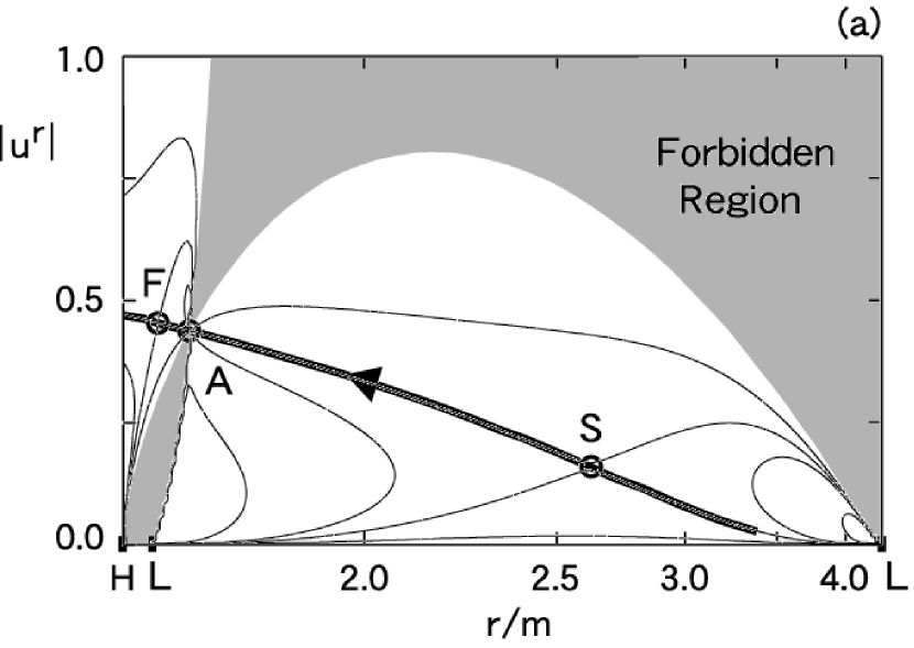
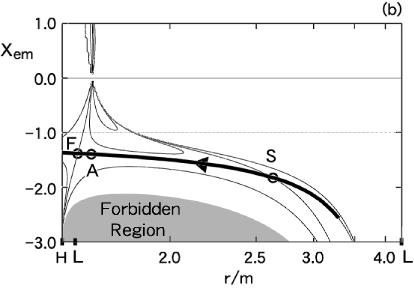
Figure 12: An example of a negative energy trans-fast MHD accretion solution (thick curves); with (a) radial 4-velocity and (b) the ratio of the electromagnetic energy to the total energy. The flow parameters are $a=0.8m$, $\Omega_{F}=0.6\Omega_{\rm max}$, $\delta=0.0$, $\Gamma=4/3$, $\zeta_{\rm F}=0.1$, $x_{\rm A}=0.95$ ($\Omega_{F}\tilde{L}=5.1710$) and $r_{\rm F}=1.647934m$, which gives $E_{\rm F}/\mu_{\rm c}=-0.15855$ and $\hat{\eta}=0.0297$.

Figure 12 shows a negative energy accretion solution ($\Omega_{F}\tilde{L}>1$). We see that the Alfvén point locates inside the ergosphere (see Paper I). The outgoing electromagnetic energy flux is always greater than the ingoing fluid energy flux ($X_{\rm em}<-1$ and $X_{\rm fluid}=-1-X_{\rm em}>0$). The magnetic field lines are trailed ($B^{\phi}/B_{p}<0$) everywhere due to the black hole rotation.

For accretion with $\Omega_{F}\tilde{L}<1$ and $0<\Omega_{F}<\omega_{\rm H}$, the electromagnetic energy flux also streams outward everywhere, but at least near the event horizon the ingoing fluid energy flux dominates [i.e., $-1<(X_{\rm em})_{\rm H}<0$]. For magnetically dominated accretion, we see that $X_{\rm em}\simeq-1$. We should mention that the Poynting flux passing through the event horizon is not modified by the plasma inertia effect, explicitly. This is because the toroidal magnetic field at the event horizon becomes $B_{\phi{\rm H}}=\sqrt{(-g_{\phi\phi}/\Sigma)_{\rm H}}\,(\omega_{\rm H}-\Omega_{F})(\partial_{\theta}\Psi)_{\rm H}$ for any ideal MHD accretion flows, which is the same expression as that of the force-free case (Znajek, 1977).

We should note that, in general, $\zeta_{\rm S}\neq\zeta_{\rm F}$ for an SAF-solution. So, when we try to estimate the locations of the fast and slow magnetosonic points for a given $\hat{\eta}$, we can only obtain possible ranges of magnetosonic points by using the $r_{\rm cr}$-$\hat{\eta}$ diagram. For example, if we know the values of $r_{\rm F}$ and $\zeta_{\rm F}$, we can find a possible region of $r_{\rm S}$ for an acceptable $\zeta_{\rm S}$ range. To determine the location of the slow magnetosonic point explicitly, we need to obtain the $\zeta_{\rm S}$ value by solving the poloidal equation, which is a polynomial with high degree.

4.3 Fluid-Dominated Flows

The solution for case (ii) becomes hydrodynamical accretion in the hydro-dominated limit. In the limit of weak magnetic field ($\varepsilon\equiv B_{p}^{2}/(8\pi P)\ll 1$), for a flow with $u_{p}^{2}(x)\sim O(\varepsilon^{0})$, we see that $M^{2}\sim O(\varepsilon^{-1})$; then, we obtain $B_{\phi}/B_{p}\sim O(\varepsilon^{0})$, $(E/\mu)=u_{t}+O(\varepsilon)$, and $(L/\mu)=-u_{\phi}+O(\varepsilon)$. The poloidal equation (10) then becomes

$$(1+u_{p}^{2})=-k\left(\frac{E}{\mu}\right)^{2}+O(\varepsilon)\ .$$ (34)

The function defined by equation (12) is reduced to $k=-g^{tt}+2g^{t\phi}\ell-g^{\phi\phi}\ell^{2}$, where $\ell\equiv-u_{\phi}/u_{t}$ is the specific angular momentum as measured at infinity. The numerator (20) and denominator (21) become

$${\cal N} = (M^{2})^{3}(1+u_{p}^{2})\left[C_{\rm sw}^{2}{\cal S}-\frac{1}{2}(1+C_{\rm sw}^{2})(\ln k)^{\prime}\right]\ ,$$ (35)

$${\cal D} = (M^{2})^{3}(C_{\rm sw}^{2}-u_{p}^{2})\ ,$$ (36)

where the function ${\cal S}={\cal S}(r,\theta)$ is related to the configuration of a stream line; for example, for a radial stream line, ${\cal S}(r)=-(2r^{2}-3mr+a^{2})/(r\Delta)$. Here, we should remember that, in the ideal MHD case, a stream line coincides with a magnetic field line. So, even for a weak magnetic field, the factor ${\cal S}$ should be related to the magnetic field lines, and in fact it must be replaced by ${\cal S}=(\ln B_{p})^{\prime}$ for MHD flows. Further, we should say that, in the weak-magnetic field limit, $\Omega_{F}$ represents the angular frequency of the stream line for a hydrodynamical flow, and it would be determined as the angular velocity of the injection point. Thus, the above expressions are reduced to the relativistic hydrodynamical flow equations formulated by Lu (1986). In equations (24), (25) and (26), we can also check that the fast magnetosonic wave speed equals the sound wave speed, while the Alfvén wave speed and the slow magnetosonic wave speed become zero.

To the contrary, for $u_{p}^{2}\sim u_{\rm AW}^{2}\sim O(\varepsilon)$, which corresponds to case (i), the hydrodynamical expression for the poloidal equation can not be obtained by a flow solution. At the Alfvén point, $M^{2}_{\rm A}=\alpha_{\rm A}\sim O(\varepsilon^{0})$ and $u_{\rm A}^{2}\sim O(\varepsilon)$. At the fast magnetosonic point, $u_{\rm F}^{2}\sim O(\varepsilon)$. So, the velocity of trans-Alfvénic MHD accretion would also be the order of $\varepsilon^{1/2}$.

5 Concluding Remarks

We have considered stationary and axisymmetric hot ideal MHD accretion along a flux-tube connected from a plasma source to the event horizon. To argue the details of the boundary conditions at the plasma source would take us beyond the scope of this paper. Therefore, we have surveyed the dependence of the trans-fast MHD flows on a wide range of source parameters. We have shown that, when the forbidden region is type IA or IIIA, there exist two physically different accretion regimes: (i) magneto-like  MHD accretion and (ii) hydro-like  MHD accretion. The magneto-like MHD accretion would be injected from near the separation point and passes through the inner Alfvén point with a smaller $\hat{\eta}$. On the other hand, the hydro-like MHD accretion with a sufficiently large $\hat{\eta}$ would be injected from between the outer Alfvén point and the outer light surface and passes through the outer Alfvén point. Hydro-like accretion may also be initially super-slow magnetosonic or super-Alfvénic. A hot ideal MHD plasma with larger $\hat{\eta}$ cannot accrete stationary onto the black hole after passing through the inner Alfvén point. Then, if the value of $\hat{\eta}$ increases with a secular timescale, the magneto-like MHD accretion solution should transit to the hydro-like MHD accretion solution; the inverse process would be also possible. The criterion for distinguishing between the two regimes is based on the locations of both the Alfvén point and the fast magnetosonic point, which change discontinuously during the transition.

For the magneto-like MHD accretion, we have found that the location of the X-type fast magnetosonic point is not unique for fixed intrinsic parameters of the accreting plasma. For example, in Figures 5a, 7b and 6, in the range of $r_{\rm H}<r_{\rm F}<r_{\rm A}^{in}$, a $\hat{\eta}=$ constant line crosses a solid curve of $\zeta_{\rm F}\leq 0.1$ at three points; the first and third fast magnetosonic points are X-type critical points, while the second one is O-type. So, we can expect two modes of magneto-like MHD accretion solutions; that is, one passes through the “inner” inner-fast magnetosonic point and the other passes through the “outer” inner-fast magnetosonic point. The number of these inner-fast magnetosonic points depends effectively on $a$, $\delta$, $\Omega_{F}$, $\tilde{L}$, $\zeta_{\rm F}$ and $\hat{\eta}$. There is a tendency for larger $\Omega_{F}-\omega_{\rm H}$ to generate a multiple inner-fast magnetosonic solution. Compared with the radial field geometry, converging field geometries for accreting flows ($\delta>0$) also generate such multiple inner-fast magnetosonic solutions. Transition between these two modes is also discontinuous. The $\delta$-dependence of SAF-accretion solutions on the flow velocity $u^{r}(r)$ and the electromagnetic energy $X_{\rm em}(r)$ is very weak, as long as the location of the fast magnetosonic point does not jump, by changing the $\delta$ value, to another branch of the multi-inner fast magnetosonic points. The radial terminal velocity at the event horizon $u^{r}_{\rm H}$, rather than the radial one, slightly decreases (increases) for $\delta>0$ ($\delta<0$). For example, we have checked this for $\delta=0.4,0.0$ and $-0.4$ cases. For such accretion solutions, we also find that for $\delta>0$ ($\delta<0$) the total energy flux per magnetic tube $\hat{\eta}E$ and $\hat{\eta}$ increase (decrease), while the total energy $E$ decreases (increases).

Throughout this paper, we have only discussed the ideal MHD flow cases. However, non-ideal MHD flow solutions near the event horizon are also presented (Punsly (1990, 2001)). Punsly (1990) discussed an ingoing magnetic flow solution along magnetic field lines that thread the ergosphere and the equatorial plane (and therefore not the event horizon). This solution corresponds to our sub-Alfvénic ingoing solution approaching the inner light surface with zero poloidal velocity (see, e.g., Fig. 10a); along this solution $B^{\phi}=0$ at $r=r_{\rm A}^{in}$ (see also, Fig. 10b), where $u_{p}^{2}\neq u_{\rm AW}^{2}$ (not the Alfvén point A), while for the SAF-solution $B^{\phi}\neq 0$ at the Alfvén point A. When we consider an accretion solution onto a black hole, it seems that there is no sub-Alfvén accretion solution consistent with the ideal MHD approximations due to the existence of the forbidden region. However, of course, for such a set of ingoing flow parameters the ideal MHD approximation must be rejected, and then the non-ideal MHD ingoing flow should exist. This is because near the light surface due to the plasma inertia effects large radiation losses are expected, and large radiation losses equate to a dissipative plasma and a breakdown of the ideal MHD approximation. Then, a non-ideal MHD accretion flow solution, which does not pass through the fast-magnetosonic critical point F discussed in the previous section, also exists in the region downstream of the light surface because of the inward attraction of black hole gravity. This requires that dissipative effects be incorporated into the physical description of the inward extension of the ideal MHD wind inside the light surface. Such a plasma propagates inside the inner light surface and enters the forbidden region of $r\leq r_{\rm L}^{in}$ with relatively slow velocity (as compared with the Alfvén wave speed except for the area close to the horizon) by crossing or reconnecting the magnetic field lines, where the physical meaning of the concept of the forbidden region for the ideal MHD flows would be lost. Note that the non-ideal MHD accretion flow must also become super-Alfvén and super-fast magnetosonic just inside the inner light surface (see Chapter 9 of Punsly 2001).

For a “super-critical” accretion flow of $E>E_{\rm F}$ and $u_{\rm AW}^{2}<u_{p}^{2}<u_{\rm FM}^{2}$, which reaches the event horizon without passing through the fast magnetosonic point F and is unphysical under the ideal MHD approximation, some kinds of dissipative effects near the event horizon would also make the super-critical accretion onto the black hole possible. One may also expect a “sub-critical” accretion flow of $E<E_{\rm F}$, which is also not a solution for the inflow into the black hole under the ideal MHD approximation. However, the breakdown of the ideal MHD would change the nature of the critical points (see, e.g., Chakrabarti (1990) for the hydrodynamical flow case); that is, instead of the X-type and O-type critical points, the “nodal-type” and “spiral-type” critical points appear on the flow solutions in the ($r,u^{r}$)-plane. Thus, when the initial condition at the plasma source does not match the critical condition at the fast magnetosonic point, the non-ideal MHD inflow into the black hole must be realized. The detailed structure of the non-ideal MHD flows around the critical point is a very important topic for black hole accretion, but further discussion is out of the scope of this paper.

When the angular velocity of the magnetosphere is in the range of $0<\Omega_{F}<\omega_{\rm H}$, only one Alfvén point appears on the $r$-$u^{r}$ plane. To accrete onto the black hole, an ideal MHD flow must pass through the Alfvén point classified by type IIAⁱⁿ, IIA^out, IIBⁱⁿ or IIB${}^{in}_{\ast}$ in Paper I. Determining whether the accretion is magneto-like or hydro-like may not be clear in type IIA case. However, we can expect that the Alfvén point Aⁱⁿ is responsible for the magneto-like accretion solution and the A^out point is responsible for the hydro-like accretion solution. It seems that for the Alfvén point of type IIB^out there are no accretion solutions consistent with the ideal MHD approximation. Of course, for such a set of ingoing flow parameters the ideal MHD approximation must be abandoned. When the SAF-accretion solution is invalid (e.g., the type IIB^out case), the non-ideal MHD accretion becomes important and would dynamically effect the magnetic field structure.

When a region of $k(r)>0$ exists along a magnetic field line for larger $\tilde{L}\Omega_{F}\,(\leq 1)$, the forbidden region is type B and the ideal MHD accretion is only allowed after passing the inner Alfvén point. The hydro-like MHD accretion does not arise because of the sufficiently strong centrifugal barrier, while the magneto-like MHD accretion is available because of the effective angular momentum transport from the fluid-part of total angular momentum to the magnetic-part (Hirotani et al. 1992). When the hot effects dominate in the plasma, this magneto-like MHD accretion may be also forbidden due to the disappearance of the inner-fast magnetosonic point. In this case, however, we can also expect the non-ideal MHD accretion to fall into the black hole.

If a shock front is generated after passing the fast magnetosonic point, the post-shock flow with increased entropy must pass another fast magnetosonic point again on the way to the event horizon. To construct such a shock formation model, the existence of multiple fast magnetosonic points is required in the accretion solution. We can expect two types of discontinuous transitions. One is the transition from the hydro-like solution to the magneto-like solution at somewhere between the middle-fast and inner-fast magnetosonic points. The other is the transition in the hydro-like or magneto-like solution. For the magneto-like solution, we can see the possibility of transition from the $r_{\rm cr}$-$\hat{\eta}$ diagrams. That is, the accreting matter passes through the first inner-fast magnetosonic point located just inside the inner-Alfvén point, and then after the shock it passes through the third (X-type) inner-fast magnetosonic point. Here, the first and third inner-fast magnetosonic points are located on different $\zeta_{\rm F}$-curves in the $r_{\rm cr}$-$\hat{\eta}$ diagram because of the entropy generation. The insights gained in the course of our analysis should be of use in further investigations of shocked accretion solutions.

Although we have discussed accretion flows onto a black hole, our treatment can be applied to outgoing flows (i.e., winds and jets). To do so, we can plot $r_{\rm cr}$-$\hat{\eta}$ diagrams in the range of $r_{\rm L}^{in}<r_{\rm cr}<\infty$ (for the fast magnetosonic point, $r_{\rm A}^{in}<r_{\rm F}<\infty$; for the slow magnetosonic point, $r_{\rm L}^{in}<r_{\rm S}<r_{\rm A}^{out}$). So, we will find the possible locations of the magnetosonic point for outflows. When the forbidden region is type IA or IIIA, we find two regimes of SAF-solutions for outflows; that is, ${\sf inj}$ $\to$ ${\sf S}^{\rm mid}$ $\to$ ${\sf A}^{out}$ $\to$ ${\sf F}^{\rm out}$ $\to$ $\infty$ and ${\sf inj}$ $\to$ ${\sf S}^{\rm in}$ $\to$ ${\sf A}^{in}$ $\to$ ${\sf F}^{\rm mid}$ $\to$ $\infty$, where the slow magnetosonic point ${\sf S}^{\rm in}$ is located between the inner light surface and the inner Alfvén point, and the fast magnetosonic point ${\sf F}^{\rm out}$ is located outside the outer Alfvén point. The former SAF-solution is also available for the type B forbidden region, and the latter SAF-solution remains in the hydrodynamical limit. From the $r_{\rm cr}$-$\hat{\eta}$ diagrams, for the outflow, the location of the fast magnetosonic points with the same $\hat{\eta}$ value strongly depends on $\delta$. A similar result has been discussed in Takahashi & Shibata (1998) as a pulsar wind model without the gravitational effects. Here, we should note that to blow away to infinity, the outgoing flows also must pass through the slow magnetosonic point and the Alfvén point, but at the asymptotic region both the super-fast and sub-fast magnetosonic outflows are available. Whether or not the outflow passes through the fast magnetosonic point depends on the field aligned parameters of flows and the geometry of field lines. So, for the outflow, the fast-magnetosonic surface does not need to cover all solid angles. We can expect that the trans-fast MHD outflow is realized at least in some part of the magnetic field lines, and the distribution of the fast-magnetosonic surface would play a very important part in explaining the generation and collimation of a highly accelerated jet or wind.

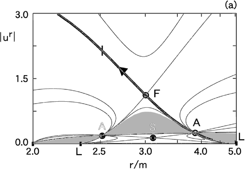
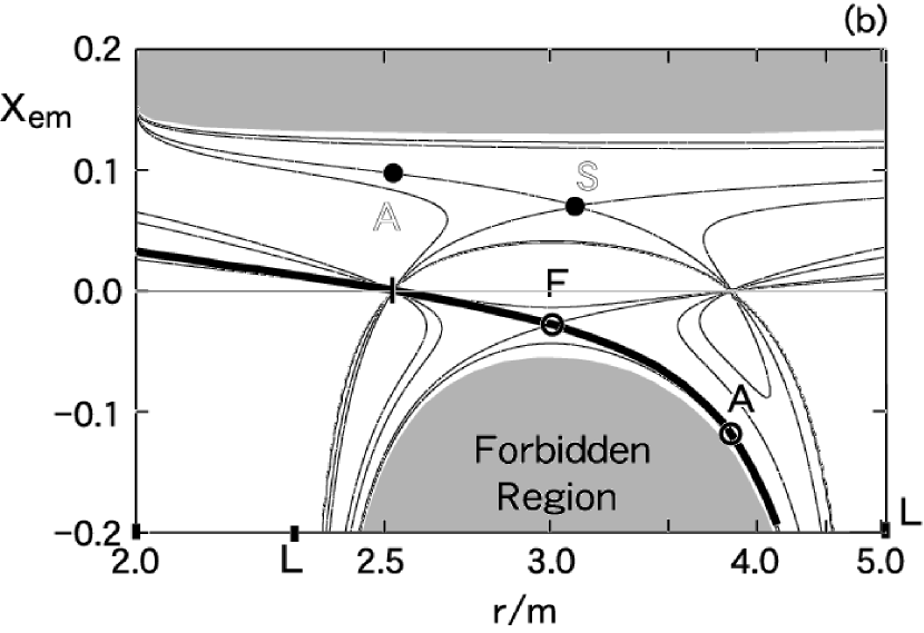
Figure 11: An example of the trans-fast MHD accretion solution (thick curves) passing through the outer Alfvén point and the middle-fast magnetosonic point; (a) radial 4-velocity and (b) the ratio of the electromagnetic energy to the total energy. The location of the fast magnetosonic point is $r_{\rm F}=3.00490m$, which gives $E_{\rm F}/\mu_{\rm c}=9.8666$ and $\hat{\eta}=0.0378$. The other parameters are the same as in Fig. 10.

References

- Abramowicz (1981) Abramowicz, M. A., and Zurek, W. H. 1981, ApJ, 246, 314
- Bekenstein (1978) Bekenstein, J. D., & Oron, E. 1978, Phys. Rev. D, 18, 1809
- Beskin (1997) Beskin, V. S. 1997, Physics-Uspekhi, 40, 659
- Blandford & Znajek (1977) Blandford, R. D., & Znajek, R. L. 1977, MNRAS, 179, 433
- Camenzind (1986a) Camenzind, M. 1986a, A&A, 156, 137
- Camenzind (1986b) Camenzind, M. 1986b, A&A, 162, 32
- Camenzind (1987) Camenzind, M. 1987, A&A, 184, 341
- Camenzind (1989) Camenzind, M. 1989, in Accretion Disks and Magnetic Fields in Astrophysics, ed. G. Belvedere (Dordrecht: Kluwer), 129
- Chakrabarti (1990) Chakrabarti, S. K., 1990, Theory of Transonic Astrophysical Flows (Singapore: World Scientific)
- Heyvaerts & Norman (1989) Heyvaerts, J., & Norman, C. 1989, ApJ, 347, 1055
- Hirotani et al. (1992) Hirotani, K., Takahashi, M., Nitta, S., & Tomimatsu, A. 1992, ApJ, 386, 455
- Kennel, Fujimura & Okamoto (1983) Kennel, C., Fujimura, F., & Okamoto, I. 1983, Geophys. Ap. Fluid Dyn., 26, 147
- Lu (1986) Lu, J.F. 1986, Gen.Rel.Grav., 18, 45
- Nitta, Takahashi, & Tomimatsu (1991) Nitta, S., Takahashi, M., & Tomimatsu, A. 1991, Phys. Rev. D, 44, 2295
- Phinney (1983) Phinney, E. S., 1983, Ph.D. thesis, Univ. Cambridge
- Punsly (1990) Punsly, B. 1990, ApJ, 354, 583
- Punsly (2001) Punsly, B. 2001, Black Hole Gravitohydromagnetics (Springer)
- Takahashi et al. (1990) Takahashi, M., Nitta, S., Tatematsu, Y., & Tomimatsu, A. 1990, ApJ, 363, 206 (Paper I)
- Takahashi (1994) Takahashi, M. 1994, in Proceedings of the Seventh Marcel Grossmann Meeting on General Relativity, ed. R. T. Jantzen, & G. M. Keiser (Singapore: World Scientific), 1298
- Takahashi & Shibata (1998) Takahashi, M., & Shibata, S. 1998, PASJ, 50, 271
- Takahashi (2000) Takahashi, M. 2000, in Proceedings of the 19th Texas Symposium on Relativistic Astrophysics and Cosmology, ed. E. Aubourg, T. Montmerle, L. Paul & P. Peter (North-Holland, Amsterdam) CD-ROM 01/27.
- Thorne, Price, & Macdonald (1986) Thorne, K. S., Price, R. H., & Macdonald, D. A., ed. 1986, Black Holes: The Membrane Paradigm (New Haven: Yale Univ. Press)
- Tomimatsu & Takahashi (2001) Tomimatsu, A., & Takahashi, M. 2001, ApJ, 552, 710
- Weber & Davis (1967) Weber, E. J., & Davis, L., Jr. 1967, ApJ, 148, 217
- Znajek (1977) Znajek, R. L. 1977, MNRAS, 179, 457