Optical and X-ray Afterglows in the Cannonball Model of GRBs

Abstract

The Cannonball Model is based on the hypothesis that GRBs and their afterglows are made in supernova explosions by relativistic ejecta similar to the ones observed in quasars and microquasars. Its predictions are simple, and analytical in fair approximations. The model describes well the properties of the $\gamma$-rays of GRBs. It gives a very simple and extremely successful description of the optical and X-ray afterglows of all GRBs of known redshift. The only problem the model has, so far, is that it is contrary to staunch orthodox beliefs.

1 Introduction

The idea that GRBs are due to collimated emissions is not recent. In the case of GRBs from quasars it was discussed by Brainerd [1]; in the case of a funnel in an explosion, by Meszaros & Rees [2]. In what is no doubt the relevant case: jets in stellar gravitational collapses, the idea has been developed over the years by Dar and collaborators [3] to [11]. Now we know that long-duration GRBs are cosmological, originate in galaxies, are associated with supernovae (SNe) and have energies that would be ridiculously large for a stellar spherical explosion (a fireball). GRBs must be “jetted”.

In the currently dominating scenarios, the ejecta that beget a GRB and its afterglow (AG) are thrown off in a uniform cone with an opening angle $\theta_{j}(0)$. This cone expands sideways: the angle $\theta_{j}(t)$ subtended by the ejecta increases with time, delineating a firetrumpet, as in Fig. (1). Relativistic jets are ubiquitous in astrophysics. The ejecta of these real jets, as seen from their emission point up to the point where they eventually stop and expand, generally subtend angles that decrease with time: just the opposite of the assumed behaviour of firetrumpets. In the analysis of the observed jets, e.g. [12, 13, 14], it is the fixed angle of observation —and not the angle subtended by the ejecta— that plays a key role.

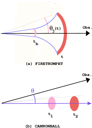
Figure 1: (a) A firecone or, more properly, a firetrumpet. In these scenarios the cone expands conically for a distance, after which the jet angle $\rm\theta_{j}$ widens faster as its firefront travels. (b) Cannonballs (shown here, somewhat pedantically, a bit Lorentz-contracted) subtend decreasing angles as they travel. The only relevant angle in the CB model is the observer’s viewing angle $\theta$.

The Cannonball (CB) model is based on the contention that GRBs and their AGs are made by relativistically jetted balls of ordinary “baryonic” matter which, by a mechanism [11] that I will outline, stop expanding soon after their emission. The CB idea gives a good description of the properties of the $\gamma$-rays in a GRB, that we modelled in simple approximations [8]. It gives an excellent and complete description of optical and X-ray afterglows, which we have modelled in full detail, as I outline here.

2 The GRB and its engine

We assume that in core-collapse SN events a tiny fraction of the parent star’s material, external to the newly-born compact object, falls back in a time of the order of very roughly one day [15, 7]. Given the considerable specific angular momentum of stars, it settles into an accretion disk around the compact object. The subsequent sudden episodes of catastrophic accretion —occurring with a chaotic time sequence that we cannot predict— result in the emission of CBs, lasting till the reservoir of accreting matter is exhausted. The emitted CBs initially expand in their rest system at a speed $\beta_{T}\,c$, of the order of the speed of sound in a relativistic plasma ($\beta_{T}=1/\sqrt{3}$). These considerations are illustrated in Fig. (2).

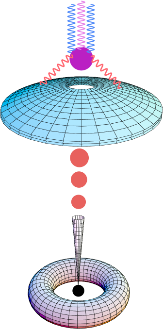
Figure 2: An “artist’s view” (not to scale) of the CB model of GRBs and their AGs. A core-collapse SN results in a compact object and a fast-rotating torus of non-ejected fallen-back material. Matter (not shown) catastrophically accreting into the central object produces a narrowly collimated beam of CBs, of which only some of the “northern” ones are depicted. As these CBs pierce the SN shell, not precisely on the same tiny spot, they heat and re-emit photons, which are Lorentz-boosted and collimated by the CBs’ relativistic motion.

From this point onwards, the CB model relies on processes whose outcome can be approximately worked out in an explicit manner. The collision of the CB with the SN shell heats the CB (which is not transparent at this point to $\gamma$’s from $\pi^{0}$ decays) to a surface temperature that, by the time the CB reaches the transparent outskirts of the SN shell, is $\sim 150$ eV, further decreasing as the CB travels [8]. The resulting quasi-thermal CB surface radiation, Doppler-shifted in energy and forward-collimated by the CB’s fast motion, gives rise to an individual pulse in a GRB [8]. The GRB light curve is an ensemble of such pulses, often overlapping one another. The energies of the individual GRB $\gamma$-rays, as well as their typical total fluences, require CB Lorentz factors $\gamma$ of ${\cal{O}}$(10³).

The CB model also explains the “Fe lines” seen in some X-ray AGs, as boosted hydrogen-recombination lines [9]. Their properties require $\gamma\sim 10^{3}$ and a baryonic number per cannonball $N_{CB}\sim 6\times 10^{50}$. Even in a GRB with very many significant pulses, the total mass of a jet of CBs would be comparable to that of the Earth: peanuts, by stellar standards.

The rest of this note is based on [11], and concentrates on afterglows, for which the CB theory is very simple.

3 Optical Afterglows: theory

When an expanding CB, in a matter of (observer’s) seconds, becomes transparent to its enclosed radiation, it loses its internal radiation pressure. If it has been expanding at a speed comparable to that of relativistic sound, should it not inertially continue to do so? No! We assume CBs to enclose a magnetic field maze, as the observed ejections from quasars and microquasars do. The interstellar medium (ISM) the CBs traverse has been previously partially ionized by the forward-beamed GRB radiation. The neutral ISM fraction is efficiently ionized by Coulomb interactions as it enters the CB. In analogy to processes occurring in quasar and microquasar ejections, the ionized ISM particles are multiply scattered, in a “collisionless” way, by the CBs’ turbulent magnetic fields. In the rest system of the CB the ISM swept-up nuclei are isotropically re-emitted, exerting an inwards force on the CB’s surface. This allows one to compute explicitly the CB’s radius as a function of time [11]. The radius, for typical parameters, reaches a constant value $R_{max}\sim 10^{14}$ cm in minutes of observer’s time.

The ISM nuclei (mainly protons) that a CB scatters also decelerate its flight: its Lorentz factor, $\gamma(t)$, is calculable. Travelling at a large $\gamma$ and viewed at a small angle $\theta$, the CB’s emissions are strongly relativistically aberrant: in minutes of observer’s time, the CBs are parsecs away from their source. For a constant CB radius and an approximately constant ISM density, $\gamma(t)$ has an explicit analytical expression [11]. Typically $\gamma=\gamma(0)/2$ at a distance of order 1 kpc from the source.

The ISM electrons entering a CB bounce off its enclosed magnetic domains, lose energy effectively by synchrotron radiation, and acquire a predictable power-law energy spectrum, $dn_{e}/dE\propto E^{-3.2}$, which implies a given distribution of the radiated photons: $\nu\,dn_{\gamma}/d\nu\propto\nu^{-1.1}$ [16]. The emitted energy rate, in a CB’s rest system, is equal to the rate at which the ISM electrons bring energy into the CB. The AG fluence in the CB model is of the form:

$$F_{\nu}=f\,\nu^{-\alpha}\;[\gamma(t)]^{2\alpha}\,\left[{2\,\gamma(t)\over 1+\gamma(t)^{2}\,\theta^{2}}\right]^{3+\alpha},$$ (1)

with $\alpha\sim 1.1$ and $f$ an explicit normalization proportional to the ISM electron density, $f\propto n_{e}$.

We assume that all long-duration GRBs are associated with SNe and, as a bold ansatz, we take these SNe to have the fluence of SN1998bw, properly transported in time and frequency to the GRB’s redshift [17]. An observed AG’s fluence is then the sum of this SN, the background galaxy emission, and the CBs’ contribution, Eq. (1). Remarkably, this very simple theory very successfully describes the optical AGs, at all times, of every GRB of known redshift.

4 X-ray afterglows: theory

In the CB model, the X-ray emission by a GRB is more complex than its optical emission. During the GRB the emitted light at all energies is mainly of thermal origin (although it does not have a thermal spectrum) and, in a fixed energy interval, it decreases exponentially with time [8]. A few seconds after the last GRB pulse (the last CB), this pseudothermal emission becomes a subdominant effect. For the next few hours, the evolution of a CB is interestingly complicated. In particular, its originally ionized material should recombine into hydrogen and emit Lyman-$\alpha$ lines that are seen Doppler-boosted to keV energies [9]. Later, the CBs settle down to a much simpler phase, which typically lasts for months, till the CBs finally stop moving relativistically.

The X-ray AG is initially dominated by thermal bremsstrahlung (TB), which has a harder spectrum than synchrotron emission. This period of TB-dominance begins at a time $t_{trans}$, a few seconds after the end of the GRB, when the last CB becomes transparent to its enclosed radiation. A few minutes later, both the X-ray and optical AGs are dominated by synchrotron radiation, and their shapes are achromatic, as in Eq. (1).

The TB X-ray fluence decreases with time as $R^{-3}\,T^{1/2}$, with $R$ the CB’s radius, still increasing linearly with time at an early stage. Depending on whether a CB’s cooling soon after $t_{trans}$ is dominated by TB, or by adiabatic losses, the X-ray fluence is $\propto t^{-5}$ or $\propto t^{-4}$, the first behaviour being expected for our typical CB parameters.

The previous considerations justify a very simple description of the X-ray light curves:

$$F_{X}(t)\simeq f_{X}(t_{trans})\,\left[{t_{trans}\over t}\right]^{5}+F_{sync}(t)\,,$$ (2)

where $t$ is the observer’s time since the ejection of the (last) CB, and $F_{sync}(t)$ is the synchrotron fluence in the X-band, i.e. Eq. (1) integrated in the relevant energy interval. The normalization $f_{X}$ is, once again, explicit in the CB model. Equation (2) provides an excellent description, at all times, of all the X-ray AGs of GRBs of known $z$.

5 Optical afterglows: results

GRBs have varied numbers, $n_{CB}$, of gamma-ray pulses, or CBs, which may have different initial Lorentz factors $\gamma_{0}$ and baryon numbers $N_{CB}$. This and other complications are eased by the fact that the AG light curve is the sum of temporally unresolved individual CB afterglows: we can characterize, as in Eq. (1), the AG with the parameters of one single CB, whose values represent a weighted average. The parameters to be fit are $f$, $\theta$ and $\alpha$ in Eq. (1), as well as two parameters entering the expression for $\gamma(t)$: $\gamma_{0}$ and the deceleration parameter $x_{\infty}\equiv N_{CB}/(\pi\,R_{max}^{2}\,n_{p})$, with $n_{p}$ the ISM proton number density light-centuries away from the GRB’s progenitor.

The fits to the CB model are generally excellent. An example, GRB 970228, is shown in Fig. (3). Our only bad fit, that to GRB 000301c, is shown in Fig. (4). The occasional misfit is to be expected: the AG fluences are proportional to $n_{e}$, which is not constant for kpc distances, even in the halo of galaxies. The fitting procedure —which attributes to the errors a counterfactual purely-statistical origin— results in tiny 1 $\sigma$ spreads for the parameters, and in excellent confidence levels, on which one should not place excessive confidence.

Figure 3: Comparison between the fitted R-band afterglow (upper curves) and the observations for GRB 970228, at $z=0.695$, without subtraction of the host galaxy’s contribution (the straight line). The contribution from a 1998bw-like supernova placed at the GRB’s redshift is indicated by a line of crosses. The SN bump is clearly discernible.

Figure 4: Comparison between the fitted R-band afterglow and the observations for GRB 000301c, at $z=2.040$, without subtraction of the host galaxy’s contribution (the straight line). The contribution from a 1998bw-like supernova placed at the GRB’s redshift is too weak to be observable.

The spectral slope in the optical-to-X-ray interval, $\alpha$, is the only parameter for which we have no reason to expect a range of different values. It is extremely satisfactory that the fitted values of $\alpha$ (extracted from the AG’s temporal shape at fixed $\nu$) are, within errors, compatible with all of the GRBs having a universal behaviour with the theoretically predicted value: $\alpha\approx 1.1$. Most spectral measurements agree with this result and, for the ones that do not (and some of the ones that do) there is always a good reason not to worry: poorly-understood absorption. The distribution of $\gamma_{0}$ values agrees snugly with our expectation from the properties of the GRB: $\gamma_{0}\sim 10^{3}$, and it is surprisingly narrow: $\Delta\gamma_{0}/\gamma_{0}\sim 0.2$. The values of $x_{\infty}$ should be fairly spread: they depend on $n_{p}$ close to the progenitor (that determines $R_{max}$) and $n_{e}$ in the region where the AG is emitted. Indeed, the $x_{\infty}$ values range for an order of magnitude above and below a typical prediction. The overall normalization $f$ of the optical afterglows is, with the other parameters fixed, $f\propto n_{CB}\,N_{CB}$. The results from optical AG fits range for an order of magnitude above and below the prediction for a single dominant CB, $n_{CB}=1$, and our typical expected $N_{CB}$. This must be partially due to absorption uncertainties, for the X-ray fits result in 1/3 as much spread.

To summarize, the distributions of all parameters are in extremely good agreement with the expectations of the CB model and, if anything, they are astonishingly close to what they would be for “standard candle” GRBs.

5.0.1 GRB 970508: a case of gravitational lensing

The AG of GRB 970508 has a most peculiar shape. An attempt to fit it with Eq. (1) is shown in Fig. (5): it is a miserable failure. But suppose the light from the CBs of this GRB is gravitationally lensed by a star or a binary, of mass $\sim 2\,M_{\odot}$, placed roughly half-way to their position (the probability for something like this to happen is a few per-cent). The lensed AG, whose CB model parameters are entirely conventional, is shown in Fig. (6): the fit is fantastically good. Comparing Figs. (5) and (6), notice how time-asymmetric the amplification is (the time scale is logarithmic!). This is because, as the lensing occurs, the CBs are — in a specific predicted fashion— slowing down from an initial superluminal speed $\rm v_{\perp}\sim 500$ c. Seing a result like this, one knows in one’s bones that one is on the right track!

Figure 5: Comparisons between a fitted R-band afterglow (upper curves) and the observations, for GRB 970508, at $z=0.835$. The galaxy has been subtracted. The fit is a total disaster.

Figure 6: The R-band AG of GRB 970508, fit with the additional effect of gravitational lensing by a $\sim 2\,M_{\odot}$ intervening object. This time the fit is excellent. A SN1998bw-like contribution is necessary.

5.0.2 GRB 990123 and its mother’s wind

For this GRB, there are good optical data starting exceptionally early: $22.18$ seconds after its detected beginning [18]. The AG rises abruptly to a second point at $t=47.38$ s, and decreases thereafter. We can very simply describe this AG from this point onwards, as shown in Fig. (7). From the fitted values of $\rm z$, $\gamma_{0}$ and $\theta$, we conclude that at that time the CBs are a mere $x=0.46$ pc away from the progenitor star. This is precisely where the density profile ought to be $n\propto r^{-2}$, induced by the parent-star’s wind and ejecta. This early, the CB’s deceleration is negligible: an $r^{-2}$ density profile implies an optical AG declining as $t^{-2}$. The shape and normalization of the early AG are precisely the expected ones (the inferred local density is $\rm 0.54\,cm^{-3}$ at $\rm x\simeq 0.46$ pc). The CB model describes the full history of an optical AG.

Figure 7: Comparisons between the fitted R-band AG and the observations, for GRB 990123, at $z=1.600$, without subtraction of the host galaxy. The data on this AG begins shortly after the GRB. The starting $t^{-2}$ behaviour is that expected if the CBs are moving trough a density profile, $n\propto r^{-2}$, induced by the parent-star’s pre-SN wind and ejections.

6 X-ray afterglows: results

Once again, I can only show a subsubset of our results. The X-ray AG of GRB 010222, and its CB-model’s description, are shown in Fig. (8). The early decline is dominated by thermal bremsstrahlung and has the expected $t^{-5}$ decline. The late AG is achromatic: the shape of the late X-ray fluence is that obtained with the parameters resulting from the fit to the optical AG. The normalizations at early and late times are in the expected range. The approximation of a constant ISM density in the normalization of $F_{sync}(t)$ in Eq. (2) should be inappropriate between $\rm\sim\!2\times 10^{-3}$ and $\sim\!0.2$ days. There are no data in that domain except for GRB 991216 and perhaps 970508, which suggest an initial density variation $\rm\propto 1/r^{2}$, resulting in an observed $\rm\sim t^{-2}$ decline, as in the optical AG of GRB 990123, shown in Fig. (7).

Our worst but most significant fit to an X-ray AG is that to GRB 980425, shown in Fig. (9). Unlike the observers [19] we assume the AG was produced by the CBs and not by conventional ejecta of the associated SN 1998bw, from which a much weaker signal is to be expected.

Figure 8: The early-time and late-time X-ray AG of GRB 010222 in the 2–10 keV, fitted with a constant density along the CB trajectory. The early decline is $\propto t^{-5}$; the late behaviour is achromatic: “parallel” to the optical AG curve.

6.1 Even GRB 980425 is “normal”

The optical AG of this close-by GRB is dominated by SN1998bw, and we have extracted its AG parameters ($\theta$, $\gamma_{0}$, etc.) from the X-ray fit of Fig. (9). The fitted viewing angle is $\theta\sim 8.3$ mrad; $\gamma_{0}\sim 750$, etc. are normal. If the CBs of GRB 980425 had been viewed from a typical viewing angle, $\theta\!\leq\!1/\gamma_{0}$, the equivalent isotropic energy would have been in the range of all other GRBs. If for this case the ISM density and CB radius were the same as for other GRBs, the predicted intensity of the X-ray “plateau” is $\rm\!\sim\!4\times 10^{-13}\,erg\,cm^{-2}\,s^{-1}$, as observed [20]. The “normal” GRB energy and X-ray AG fluence strongly support the association of SN1998bw with (a not exceptional) GRB 980425.

Figure 9: CB-model fit to the X-ray afterglow of the SN1998bw/GRB 980425 pair. The flatish domain we call “plateau”. It is so extensive because $\theta\,\gamma_{0}\gg 1$ and it takes time to reach the maximum at $\theta\,\gamma(t)\sim 1$.

The parameters of the X-ray AG can be used to predict the magnitude and shape of the optical AG of the blended SN 1998bw/GRB 980425 system, see Fig. (10). The CBs’ contribution dominates at late time and is in perfect agreement with the HST observation [22] on day 778. At that time the SN and the CB (this is a single-pulse GRB) were far enough from each other, and close enough to us, to be resolvable! [7]. Alas, the rare occasion was missed.

Interpreted in the CB model, the fluence and soft spectrum of GRB980425, as well as its X-ray and optical AGs were “normal”. It was simply much closer, and viewed at a much larger angle than other GRBs.

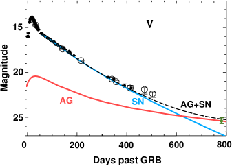
Figure 10: The V-band light curve of SN1998bw/GRB 980425. The blue “SN” curve is a fit to the SN [21], dominated after day $\sim\!40$ by ⁵⁶Co decay. The red “AG” curve is our prediction for the CB-induced AG component, as given by Eq. (1), with the parameters determined from the X-ray AG fit in the previous figure. The SN contribution dominates up to day $\sim\!600$. The last point is an HST measurement at day 778, that precisely agrees with the (dashed) SN plus CB prediction for the total AG.

Figure 11: Comparisons between our fitted R-band afterglow and the observations for GRB 000418, at $\rm z=1.119$. The galaxy has been subtracted. The contribution from a 1998bw-like SN placed at the GRB’s redshift is indicated by a line of crosses. There is a significant indication of a SN1998bw-like contribution.

Figure 12: The same as Fig. (11), but for GRB 980613, at $\rm z=1.096$. A SN 1998bw-like contribution, though based on only one significant point, appears to be required.

Figure 13: The same as Fig. (11), but for GRB 991216, at $\rm z=1.020$. The data show possible evidence for a SN bump.

Figure 14: The same as Fig. (11), but for GRB 980703, at $\rm z=0.966$. A SN 1998bw-like contribution, though the errors are large, appears to be required.

Figure 15: The same as Fig. (11), but for GRB 991208, at $\rm z=0.706$. The SN contribution is clearly discernible.

Figure 16: The same as Fig. (11), but for GRB 990712, at $\rm z=0.434$. The SN contribution is clearly discernible, but a bump at slightly earlier times than that of our standard-candle SN1998bw would provide a slightly better description.

6.2 Are GRBs associated with SNe?

The complete success of the CB model in describing optical AGs results in an excellent exposition [11] of the GRB/SN association. It is useful to discuss the issue in order of diminishing redshift. In the six more distant GRBs there is no evidence for or against a SN 1998bw-like component, two examples are given in Figs. (4) and (7). In the next five closer cases there is evidence, ranging from fairly weak to very strong; see Fig. (6) for GRB 970508, for which the light curve —in the CB model— clearly requires a SN component. The other seven of these cases —000418, 980613, 991216, 980703, 991208, and 990712, shown in Figs. (11) to (16) and 970228, shown in Fig.(3)— a SN1998bw-like contribution is required, to varying levels of statistical confidence. Finally, GRB 980425, at $z=0.0085$ is indeed associated to a SN [23]. The general trend is clear. With its excellent description of afterglows, the CB model’s predictions for the “proper” AG from the CBs provide an excellent “background” on top of which to discern a SN contribution. The conclusion is that, the closer a GRB is, the better the evidence for a SN. For the more distant GRBs, a SN could not be seen, even if it was there. In all cases where the SN could be seen, it was seen; the evidence gaining in significance as the distance diminishes. The conclusion that all long-duration GRBs are associated with SNe is irresistible.

6.3 What fraction of SNe emit GRBs?

The $\gamma$-ray fluence of a GRB [7] is $\propto[2\,\gamma_{0}/(1+\gamma_{0}^{2}\,\theta^{2})]^{3}$. The $\theta$ dependence is the steepest parameter dependence of the CB model. It is reasonable to attribute the range of equivalent spherical energies mainly to the $\theta$ dependence (as if GRBs were otherwise standard candles). Excepting GRB 980425, the observed spread in equivalent energy then corresponds to a spread $\theta\approx 0$ to $\theta_{max}\approx 2.4/\gamma$. Thus the fraction of observable GRBs (with the current or past sensitivity) is $f(\gamma)=2\pi\,\theta_{max}^{2}/(4\pi)\approx 2.84/\gamma^{2}$, with two jets of CBs per event. The rate of Type II/Ib/Ic SNe in the observable universe, multiplied by $f(10^{3})$, coincides with the observed rate of GRBs, as if every SN emitted GRBs! But the observational errors are very large; distant SNe may be more frequent than in current estimates, if the star formation rate continues to increase above $z\sim 1$; the efficiency of GRB detection as a function of fluence has not been taken into account in this estimate. In spite of these uncertainties, the conclusion, in the CB model, is that a very large fraction of SNe emit GRBs. Then, why is SN1998bw peculiar? We have seen that in X-rays it is not: they were CB-induced. Other peculiarities should also be due to how close to the GRB “axis” this SN was observed.

7 Conclusions and social affairs

At the time I gave this talk and submitted it to the Woods Hole GRB conference proceedings, we had not yet worked out the CB-model’s predictions for radio afterglows. By the time I am posting it on the web, we have made significant progress: once again, the CB model’s predictions are uncharacteristically simple and succesful [25]. We have no CB-model explanation for the scintillation behaviour of GRB 970508 [24]. Other than that, the CB model explains well all properties of GRBs. In the case of optical and X-ray afterglows, which I have outlined, the CB-model’s predictions are univocal (as opposed to multiple-choice), very explicit, analytical in fair approximations, quite simple, very complete, and extremely successful. I doubt that this statement applies to other models of GRBs.

I am not saying that the CB model will stand all future tests. But I would expect that —confronted with a simple and successful model— most scientists would, at least, say: Hum! and ask good questions. Not the case. Four of our papers on this subject, [7] to [10], have already been rejected by referees who found no single error, and/or stuck to bad numerical questions, even after being proved numerically (i.e. inarguably) wrong. This rejection statistics makes me feel that the GRB community has officially certified us… as crackpots. All this reflects, I suspect, the global rise of fundamentalism. Some people, almost literally in this case, still refuse to “look through the telescope”. A GRB theorist, sitting on the first row in my talk, was kind enough to enact my social comments. Indeed, he rose in ire to exclaim: I am glad that the referee system is working! He then stuck to a bad numerical question. Most of the rest of the questions period was not this aggressive: there is still hope in science’s sempiternal contest with faith.

References

- [1] Brainerd J.J., ApJ, 394, 33L (1992).
- [2] Meszaros P., Rees M.J., MNRAS, 257, 29P (1992).
- [3] Shaviv N.J., Dar A., ApJ, 447, 863 (1995).
- [4] Dar A., 1997, astro-ph/9704187.
- [5] Dar A., ApJ, 500, L93 (1998).
- [6] Dar A., Plaga R., A&A, 349, 259 (1999).
- [7] Dar A., De Rújula, A., astro-ph/0008474, rejected by A&A.
- [8] Dar A., De Rújula, A., astro-ph/0012227, rejected by A&A.
- [9] Dar A., De Rújula, A., astro-ph/0102115, rejected by A&A.
- [10] Dar A., De Rújula, A., astro-ph/0105094, rejected by Phys. Rev.
- [11] Dado, S., Dar A., De Rújula, A., astro-ph/0107367, submitted to A&A.
- [12] Pearsons T.J., Zensus J.A., 1987, Superluminal Radio Sources, Cambridge Univ. Press 1987, pp. 1.
- [13] Mirabel I.F., Rodriguez L.F., Nature, 371, 46 (1994); ARA&A, 37, 409 (1999).
- [14] Ghisellini G., Celotti A., astro-ph/0103007.
- [15] De Rújula A., Phys. Lett., 193, 514 (1987).
- [16] Dar A., De Rújula, A., MNRAS, 323, 391 (2001).
- [17] Dar A., GCN Circ., 346 (1999).
- [18] Akerlof C., et al., Nature, 398, 400 (1999).
- [19] Pian E., et al., A&AS, 138(3), 463 (1999).
- [20] Pian E., et al., A&A, 372, 456 (2001).
- [21] Sollerman J., et al., astro-ph/0006406
- [22] Fynbo J.U., et al., ApJ, 542, 89L (2000).
- [23] Galama T.J., et al., Nature, 395, 670 (1998).
- [24] Taylor G.J., et al., Nature, 389, 263 (1997).
- [25] Dado, S., Dar A., De Rújula, A., to be posted in the Archives.