Dynamical Simulations of Magnetically Channeled Line-Driven Stellar Winds: I. Isothermal, Nonrotating, Radially Driven Flow

Abstract

We present numerical magnetohydrodynamic (MHD) simulations of the effect of stellar dipole magnetic fields on line-driven wind outflows from hot, luminous stars. Unlike previous fixed-field analyses, the simulations here take full account of the dynamical competition between field and flow, and thus apply to a full range of magnetic field strength, and within both closed and open magnetic topologies. A key result is that the overall degree to which the wind is influenced by the field depends largely on a single, dimensionless, ‘wind magnetic confinement parameter’, $\eta_{\ast}$ ($=B_{eq}^{2}R_{\ast}^{2}/{\dot{M}}v_{\infty}$), which characterizes the ratio between magnetic field energy density and kinetic energy density of the wind. For weak confinement $\eta_{\ast}\leq 1$, the field is fully opened by the wind outflow, but nonetheless for confinements as small as $\eta_{\ast}=1/10$ can have a significant back-influence in enhancing the density and reducing the flow speed near the magnetic equator. For stronger confinement $\eta_{\ast}>1$, the magnetic field remains closed over a limited range of latitude and height about the equatorial surface, but eventually is opened into a nearly radial configuration at large radii. Within closed loops, the flow is channeled toward loop tops into shock collisions that are strong enough to produce hard X-rays, with the stagnated material then pulled by gravity back onto the star in quite complex and variable inflow patterns. Within open field flow, the equatorial channeling leads to oblique shocks that are again strong enough to produce X-rays, and also lead to a thin, dense, slowly outflowing ‘disk’ at the magnetic equator. The polar flow is characterized by a faster-than-radial expansion that is more gradual than anticipated in previous 1D flow-tube analyses, and leads to a much more modest increase in terminal speed ($<30\%$), consistent with observational constraints. Overall, the results here provide a dynamical groundwork for interpreting many types of observations – e.g., UV line profile variability; red-shifted absorption or emission features; enhanced density-squared emission; X-ray emission – that might be associated with perturbation of hot-star winds by surface magnetic fields.

1 Introduction

Hot, luminous, OB-type stars have strong stellar winds, with asymptotic flow speeds up to $v_{\infty}\sim 3000$ km/s and mass loss rates up to ${\dot{M}}\sim 10^{-5}M_{\odot}$ /yr. These general properties are well-explained by modern extensions (e.g. Pauldrach, Puls, and Kudritzki 1986) of the basic formalism developed by Castor, Abbott, and Klein (1975; hereafter CAK) for wind driving by scattering of the star’s continuum radiation in a large ensemble of spectral lines.

However there is also extensive evidence that such winds are not the steady, smooth outflows envisioned in these spherically symmetric, time-independent, CAK-type models, but instead have extensive structure and variability on a range of spatial and temporal scales. Relatively small-scale, stochastic structure – e.g. as evidenced by often quite constant soft X-ray emission (Long & White 1980), or by UV lines with extended black troughs understood to be a signature of a nonmonotonic velocity field (Lucy 1982) – seems most likely a natural result of the strong, intrinsic instability of the line-driving mechanism itself (Owocki 1994; Feldmeier 1995). But larger-scale structure – e.g. as evidence by explicit UV line profile variability in even low signal-to-noise IUE spectra (Kaper et al. 1996; Howarth & Smith 1995) – seems instead likely to be the consequence of wind perturbation by processes occurring in the underlying star. For example, the photospheric spectra of many hot stars show evidence of radial and/or non-radial pulsation, and in a few cases there is evidence linking this with observed variability in UV wind lines (Telting, Aerts, & Mathias 1997; Mathias et al. 2001).

An alternate scenario – one explored through dynamical simulations here – is that, in at least some hot stars, surface magnetic fields could perturb, and perhaps even channel, the wind outflow, leading to rotational modulation of wind structure that is diagnosed in UV line profiles, and perhaps even to magnetically confined wind-shocks with velocities sufficient to produce the relatively hard X-ray emission seen in some hot-stars.

The sun provides a vivid example of how a stellar wind can be substantially influenced by a surface magnetic field. Both white-light and X-ray pictures show the solar corona to be highly structured, with dense loops where the magnetic field confines the coronal gas, and low-density coronal holes where the more radial magnetic field allows a high-speed, pressure-driven, coronal outflow (Zirker 1977). In a seminal paper, Pneuman and Kopp (1971) provided the first magnetohydrodynamical (MHD) model of this competition between magnetic confinement and coronal expansion. Using an iterative scheme to solve the relevant partial differential equations for field and flow, they showed that this competition leads naturally to the commonly observed ‘helmet’ streamer configuration, for which the field above closed magnetic loops is extended radially outward by the wind outflow. Nowadays such MHD processes can be readily modelled using time-dependent MHD simulation codes, such as the Versatile Advection Code (Keppens and Goedbloed 1999), or the publicly available ZEUS codes (Stone and Norman 1992). Here we apply the latter to study MHD processes within line-driven stellar winds that have many characteristics quite distinct from the pressure-driven solar wind.

For the solar wind, the acceleration to supersonic speeds can take several solar radii; as such, magnetic loops that typically close within a solar radius or so can generally maintain the coronal gas in a nearly hydrostatic configuration. As we show below, in the more rapid line-acceleration of hot-stars winds, strong magnetic confinement typically channels an already supersonic outflow, often leading to strong shocks where material originating from different footpoints is forced to collide, with compressed material generally falling back to the star in quite complex and chaotic patterns. In the solar wind, the very low mass-loss-rate, and thus the low gas density and pressure, mean that only a modest magnetic field strength, of order of a Gauss, is sufficient to cause significant confinement and channeling of the coronal expansion. In hot-star winds, magnetic confinement or channeling generally requires a much stronger magnetic field, on the order of hundreds of Gauss. As such, a key issue underlying the study here regards the theoretical prospects and observational evidence for hot-star magnetic fields of this magnitude.

In the sun and other cool stars, magnetic fields are understood to be generated through a dynamo mechanism, in which coriolis forces associated with stellar rotation deflect convective motions in the hydrogen and helium recombination zones. In hot stars, hydrogen remains fully ionized even through the atmosphere, and so, lacking the strong convection zones associated with hydrogren recombination, such stars have traditionally been considered not to have strong, dynamo-generated magnetic fields. However, considering the generally quite rapid rotation of most hot stars, dynamo-generation may still be possible, e.g. within thin, weaker, near-surface convection zones associated with recombination of fully ionized helium.

Moreover, the interior, energy-generation cores of such massive stars are thought to have strong convection, and recently Cassinelli and Macgregor (2000; see also Charbonneau and MacGregor 2001) have proposed that dynamo-generated magnetic flux tubes from this interior could become buoyant, and thus drive an upward diffusion to the surface over a time-scale of a few million years. Such a model would predict surface appearance of magnetic fields in hot-stars that have evolved somewhat from the zero-age-main sequence. Alternatively, magnetic fields could form from an early, convective phase during the star’s initial formation, or perhaps even arise through compression of interstellar magnetic flux during the initial stellar collapse. Such primordial models would thus predict magnetic fields to be strongest in the youngest stars, with then some gradual decay as the star evolves.

In recent years there has been considerable effort to develop new techniques (e.g., based on the Hanle effect; Ignace, Nordsieck, & Cassinelli 1997; Ignace, Cassinelli, & Nordsieck 1999) to observationally detect stellar magnetic fields. But the most direct and well-demonstrated method is through the Zeeman splitting and associated circular polarization of stellar photospheric absorption lines (Borra & Landstreet 1980). This technique has been used extensively in direct measurement of the quite strong magnetic fields that occur in the chemically peculiar Ap and Bp stars (Babcock 1960; Borra et al. 1980; Bohlender 1993; Mathys 1995; Mathys et al. 1997). For more ‘normal’ (i.e., chemically non-peculiar) hot stars, the generally strong rotational line-broadening severely hinders the direct spectropolarimetric detection of their generally much weaker fields, yielding instead mostly only upper limits, typically of order a few hundred Gauss. This, coincidentally and quite tantalizingly, is similar to the level at which magnetic fields can be expected to become dynamically significant for channeling the wind outflow.

Recently, however, there have been first reports of positive field detections in a few normal hot stars. For the relatively slowly rotating star $\beta$ Cephei, Henrichs et al. (2000) and Donati et al. (2001) report a 3-sigma detection of a ca. 400 G dipole field, with moreover a rotational modulation suggesting the magnetic axis is tilted to be nearly perpendicular to the stellar rotation. There are also initial reports (Donati 2001) of a ca. 1000 G dipole field in $\theta^{1}$ Ori C, this time with the magnetic axis tilted by about 45 degrees to the rotation. For Ap and Bp stars, the most generally favored explanation for their strong fields is that they may be primordial, and the relative youth of $\theta^{1}$ Ori C also seems to suggest a primordial model. In contrast, the more evolved evolutionary status of $\beta$ Cephei seems to favor the interior-eruption scenario.

The focus of the present paper is to carry out magnetohydrodynamical simulations of how such magnetic fields on the surface of hot stars can influence their radiatively driven stellar wind. Our approach here represents a natural extension of the previous studies by Babel & Montmerle (1997a,b; hereafter BM97a,b), which effectively prescribed a fixed magnetic field geometry to channel the wind outflow. For large magnetic loops, wind material from opposite footpoints is accelerated to a substantial fraction of the wind terminal speed (i.e. $\sim 1000$ km/s) before the channeling toward the loop tops forces a collision with very strong shocks, thereby heating the gas to temperatures ($10^{7}-10^{8}$ K) that are high enough to emit hard (few keV) X-rays. This ‘magnetically confined wind shock’ (MCWS) model was initially used to explain X-ray emission from the Ap-Bp star IQ Aur (BM97a), which has a quite strong magnetic field ($\sim 4$kG) and a rather weak wind (mass loss rate $\sim 10^{-10}M_{\odot}/$ yr), and thus can indeed be reasonably modeled within the framework of prescribed magnetic field geometry. Later, BM97b applied this model to explain the periodic variation of X-ray emission of the O7 star $\theta^{1}$ Ori C, which has a much lower magnetic field ($\mathrel{\hbox to0.0pt{\lower 3.0pt\hbox{$\mathchar 536\relax$}\hss}\raise 2.0pt\hbox{$\mathchar 316\relax$}}1000$ G) and significantly stronger wind (mass loss rate $\sim 10^{-7}M_{\odot}/$ yr), raising now the possibilty that the wind itself could influence the field geometry in a way that is not considered in the simple fixed-field approach.

The simulation models here are based on an isothermal approximation of the complex energy balance, and so can provide only a rough estimate of the level of shock heating and X-ray generation. But a key advantage over previous approaches is that these models do allow for such a fully dynamical competition between the field and flow. A central result is that the overall effectiveness of magnetic field in channeling the wind outflow can be well characterized in terms of single ‘wind magnetic confinement parameter’ $\eta_{\ast}$, defined in eqn. (7) below, and related to the relative energy densities of field and wind (§3). The specifics of our numerical MHD method are described in §2, while §4 details the results of a general parameter study of hot-star winds with various degrees of magetic confinement. Following a discussion (§5) of the implications of these results for modeling hot-star wind structure and variability, we finally conclude (§6) with a summary and outlook for future work.

2 Numerical Method

2.1 Magnetoydrodynamic Equations

Our general approach is to use the ZEUS-3D (Stone and Norman 1992) numerical MHD code to evolve a consistent dynamical solution for a line-driven stellar wind from a star with a dipolar surface field. As described further below, the basic ZEUS-3D code was modified for the present study to include radiative driving terms, and to allow for specification of the lower boundary conditions. The code is designed to be easily adapted to run in a variety of flow geometries (planar, cylindrical, spherical) in one, two, or three dimensions. Our implementation here uses spherical polar coordinates with radius $r$, co-latitude $\theta$, and azimuth $\phi$ in a 2D formulation, which assumes all quantites are constant in azimuthal angle $\phi$, and that the azimuthal components of both field and flow vanish, $B_{\phi}=v_{\phi}=0$.

The time-dependent equations to be numerically integrated thus include the conservation of mass,

$$\frac{D\rho}{Dt}+\rho\nabla\cdot{\bf v}=0,$$ (1)

and the equation of motion

$$\rho\frac{D{\bf v}}{Dt}=-\nabla p+\frac{1}{4\pi}(\nabla\times{\bf B})\times{\bf B}-{GM(1-\Gamma){\hat{\bf r}}\over r^{2}}+{\bf g}_{lines},$$ (2)

where $\rho$, $p$, and ${\bf v}$ are the mass density, gas pressure, and velocity of the fluid flow, and $D/Dt=\partial/\partial t+{\bf v}\cdot\nabla$ is the advective time derivative. The gravitational constant $G$ and stellar mass $M$ set the radially directed (${\hat{\bf r}}$) gravitational acceleration, and $\Gamma\equiv\kappa_{e}L/(4\pi GMc)$ is the Eddington parameter, which accounts for the acceleration due to scattering of the stellar luminosity $L$ by free electron opacity $\kappa_{e}$, with $c$ the speed of light. The additional radiative acceleration due to line scattering, ${\bf g}_{lines}$, is discussed further below. The magnetic field ${\bf B}$ is constrained to be divergence free

$$\nabla\cdot{\bf B}=0,$$ (3)

and, under our assumption of an idealized MHD flow with infinite conductivity (e.g. Priest & Hood 1991), its inductive generation is described by

$$\frac{\partial{\bf B}}{\partial t}=\nabla\times({\bf v}\times{\bf B}).$$ (4)

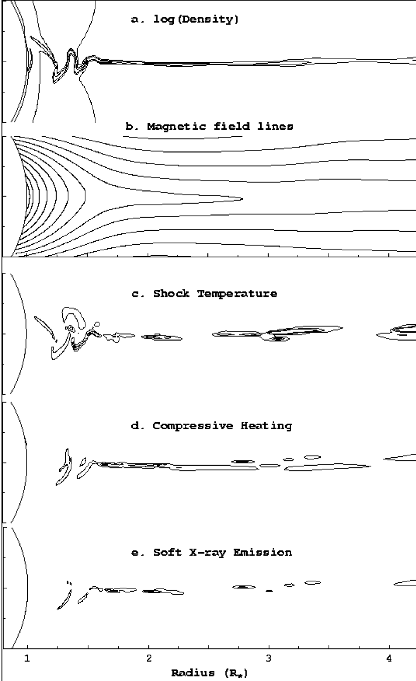
Figure 9: For the strong magnetic confinement case $\eta_{\ast}=10$, contours of a. log(density), b. magnetic field lines, c. shock temperature [estimated from eqn. (12)], d. compressive heating [computed from eqn.(13)], and e. soft X-ray emission [estimated from eqn. (14), with $E=0.1$ keV]. The 3 contour levels correspond to $\log(\rho)=$ -12, -13, and -14 ($g/cm^{3}$) in panel a; to $T_{s}=$ 1, 11, and 21 MK in panel b; and to $q$ (or $q_{E}$) of 0.15, 0.9, and 1.5 erg/cm³/s in panels c and d.

The ZEUS-3D code can also include an explicit equation for conservation of energy, but in the dense stellar winds considered here, the energy balance is dominated by radiative processes that tend to keep the wind near the stellar effective temperature $T_{eff}$ ( Drew 1989; Pauldrach 1987). In this initial study, we assume an explicitly isothermal flow with $T=T_{eff}$, which thus implies a constant sound speed $a=\sqrt{kT/m}$, with $k$ Boltzmann’s constant and $m$ the mean atomic weight of the gas. The perfect gas law then gives the pressure as $p=\rho a^{2}$. In such an isothermal model, even the locally strong compressive heating that occurs near shocks is assumed to be radiated away within a narrow, unresolved cooling layer (Castor 1987; Feldmeier et al. 1997; Cooper 1994). We thus defer to future work the quantitative modeling of the possible EUV and X-ray emission of any such shocks, although below (§5.3.4) we do use computed velocity jumps to provide rough estimates of the expected intensity and hardness of such shock emissions. (See figure 9.)

2.2 Spherically Symmetric Approximation for Radial Line-Force

The radiative acceleration ${\bf g}_{lines}$ results from scattering of the stellar radiation in a large ensemble of spectral lines. In these highly supersonic winds this can be modeled within the framework of the Sobolev (1960) approximation as depending primarily on the local velocity gradient averaged over the directions of the source radiation from the stellar disk. For 1D nonrotating winds, the line-force-per-unit-mass can be written in the form (cf. Abbott 1982; Gayley 1995)

$$g_{lines}=\frac{f}{(1-\alpha)}~{}\frac{\kappa_{e}L{\bar{Q}}}{4\pi r^{2}c}\left(\frac{dv/dr}{\rho c\bar{Q}\kappa_{e}}\right)^{\alpha}$$ (5)

where $\alpha$ is the CAK exponent, and $f$ is the (1D) finite disk correction factor, given by CAK eqn. (50). (See also Friend and Abbott 1986, and Pauldrach, Puls, and Kudritzki 1986.) Here we choose to follow the Gayley (1995) line-distribution normalization $\bar{Q}$, which offers the advantages of being a dimensionless measure of line-opacity that is independent of the assumed ion thermal speed $v_{th}$, and with a nearly constant characteristic value of order ${\bar{Q}}\sim 10^{3}$ for a wide range of ionization conditions (Gayley 1995). This normalization is related to the ususal CAK parameter through $k={\bar{Q}}^{1-\alpha}\,\left(v_{th}/c\right)^{\alpha}/(1-\alpha)$.

In the 2D wind models computed here, the line force (5) should in principle be modified to take account of gradients in other velocity components, such as might arise from, e.g., latitudinal flow along magnetic loops. Such latitudinal gradients can modify the form of the radial finite-disk correction factor $f$, and can even lead to a non-zero latitudinal component of the full vector line force. In a rotating stellar wind, asymmetries in the velocity gradient between the approaching and receding stellar hemisphere can even lead to a net azimuthal line force (Owocki, Cranmer, and Gayley 1996; Gayley and Owocki 2000). For simplicity, we defer study of such rotational and latitudinal affects to future work, and thus apply here just the radial, 1D form (5) for the line force, within a 2D, axisymmetric model of a non-rotating stellar wind.

2.3 Numerical Specifications

Let us next describe some specifics of our numerical discretization and boundary conditions. In our implementation of the ZEUS MHD code, flow variables are specifed on a fixed 2D spatial mesh in radius and co-latitude, $\{r_{i},\theta_{j}\}$. The mesh in radius is defined from an initial zone $i=1$, which has a left interface at $r_{1}=R_{\ast}$, the star’s surface radius, out to a maximum zone ($i=n_{r}=300$), which has a right interface at $r_{301}=6R_{\ast}$. Near the stellar base, where the flow gradients are steepest, the radial grid has an initially fine spacing with $\Delta r_{1}=0.00026R_{\ast}$, and then increases by 2% per zone out to a maximum of $\Delta r_{299}=0.11R_{\ast}$.

The mesh in co-latitude uses $n_{\theta}=100$ zones to span the two hemispheres from one pole, where the $j=1$ zone has a left interface at $\theta_{1}=0\arcdeg$, to the other pole, where the $j=n_{\theta}=100$ zone has a right interface at $\theta_{101}=180\arcdeg$. To facilitate resolution of compressed flow structure near the magnetic equator at $\theta=90\arcdeg$, the zone spacing has a minimum of $\Delta\theta_{50}=0.29\arcdeg$ at the equator, and then increases by 5% per zone toward each pole, where $\Delta\theta_{1}=\Delta\theta_{100}=5.5\arcdeg$. Test runs with half the resolution in radius and/or latitude showed some correspondingly reduced detail in flow fine-structure, but overall the results were qualitatively similar to those for the standard resolution.

Our operation uses the piecewise-linear-advection option within ZEUS (VanLeer 1977), with time steps set to a factor 0.30 of the minimum MHD Courant time computed within the code (Courant et al. 1953). Boundary conditions are implemented by specification of variables in two phantom zones. At both poles, these are set by simple reflection about the boundary interface. At the outer radius, the flow is invariably super-Afvenic outward, and so outer boundary conditions for all variables (i.e. density, and the radial and latitutudinal components of both the velocity and magnetic field) are set by simple extrapolation assuming constant gradients.

The boundary conditions at the stellar surface are specified as follows. In the two radial zones below $i=1$, we set the radial velocity $v_{r}$ by constant-slope extrapolation, and fix the density at a value $\rho_{o}$ chosen to ensure subsonic base outflow for the characteristic mass flux of a 1D, nonmagnetic CAK model, i.e. $\rho_{o}\approx{\dot{M}}/(4\pi R_{\ast}^{2}a/5)$. Detailed values for each model case are given in Table 1. In our 2D magnetic models, these conditions allow the mass flux and the radial velocity to adjust to whatever is appropriate for the local overlying flow (Owocki, Castor, and Rybicki 1988). In most zones, this corresponds to a subsonic wind outflow, although inflow at up to the sound speed is also allowed.

Magnetic flux is introduced through the radial boundary as the radial component of a dipole field $B_{r}(R_{\ast})=B_{o}\cos(\theta)$, where the assumed polar field $B_{o}$ is a fixed parameter for each model (see Table 1). The latitudinal component of magnetic field, $B_{\theta}$, is set by constant slope extrapolation. The specification for the latitudinal velocity, $v_{\theta}$, differs for strong vs. weak field cases. For strong fields (defined by the magnetic confinement parameter $\eta_{\ast}>1$; see §3), we again use linear extrapolation. (We also find similar results using $v_{\theta}=v_{r}B_{\theta}/B_{r}$.) For weak fields ($\eta_{\ast}\leq 1$), we simply set $v_{\theta}=0$. Tests using each approach in the intermediate field strength case ($\eta_{\ast}=1$) gave similar overall results.

This time-dependent calculation also requires us to specify an initial condition for each of these flow variables over the entire spatial mesh at some starting time $t=0$. The hydrodynamical flow variables $\rho$ and ${\bf v}$ are initialized to values for a spherically symmetric, steady, radial CAK wind, computed from relaxing a 1D, non-magnetic, wind simulation to an asymptotic steady state. The magnetic field is initilized to have a simple dipole form with components $B_{r}=B_{o}(R_{\ast}/r)^{3}\cos\theta$, $B_{\theta}=(B_{o}/2)(R_{\ast}/r)^{3}\sin\theta$, and $B_{\phi}=0$, with $B_{o}$ the polar field strength at the stellar surface. From this initial condition, the numerical model is then evolved forward in time to study the dynamical competition between the field and flow. The results of such dynamical simulations are described in §4.

3 Heuristic Scaling Analysis for Field vs. Flow Competition

3.1 The Wind Magnetic Confinement Parameter

To provide a conceptual framework for interpreting our MHD simulations, let us first carry out a heuristic scaling analysis of the competition between field and flow. To begin, let us define a characteristic parameter for the relative effectiveness of the magnetic fields in confining and/or channeling the wind outflow. Specifically, consider the ratio between the energy densities of field vs. flow,

$$\eta(r,\theta) \equiv \frac{B^{2}/8\pi}{\rho v^{2}/2}$$

$$\approx \frac{B^{2}r^{2}}{\dot{M}v}$$

$$= \left[\frac{B_{\ast}^{2}(\theta){R_{\ast}}^{2}}{\dot{M}v_{\infty}}\right]\left[\frac{(r/R_{\ast})^{2-2q}}{1-R_{\ast}/r}\right]\,,$$

where the latitudinal variation of the surface field has the dipole form given by $B_{\ast}^{2}(\theta)=B_{o}^{2}(\cos^{2}\theta+\sin^{2}\theta/4)$. In general, a magnetically channeled outflow will have a complex flow geometry, but for convenience, the second equality in eqn. (3.1) simply characterizes the wind strength in terms of a spherically symmetric mass loss rate $\dot{M}=4\pi r^{2}\rho v$. The third equality likewise characterizes the radial variation of outflow velocity in terms of the phenomenological velocity law $v(r)=v_{\infty}(1-R_{\ast}/r)$, with $v_{\infty}$ the wind terminal speed; this equation furthermore models the magnetic field strength decline as a power-law in radius, $B(r)=B_{\ast}(R_{\ast}/r)^{q}$, where, e.g., for a simple dipole $q=3$.

With the spatial variations of this energy ratio thus isolated within the right square bracket, we see that the left square bracket represents a dimensionless constant that characterizes the overall relative strength of field vs. wind. Evaluating this in the region of the magnetic equator ($\theta=90\arcdeg$), where the tendency toward a radial wind outflow is in most direct competition with the tendency for a horizontal orientation of the field, we can thus define a equatorial ‘wind magnetic confinement parameter’,

$$\eta_{\ast} \equiv \frac{B_{\ast}^{2}(90\arcdeg){R_{\ast}}^{2}}{\dot{M}v_{\infty}}$$ (7)

$$= 0.4\,\frac{B_{100}^{2}\,R_{12}^{2}}{\dot{M}_{-6}\,v_{8}}.$$

where $\dot{M}_{-6}\equiv\dot{M}/(10^{-6}\,M_{\odot}$/yr), $B_{100}\equiv B_{o}/(100$ G), $R_{12}\equiv R_{\ast}/(10^{12}$ cm), and $v_{8}\equiv v_{\infty}/(10^{8}$ cm/s). As these stellar and wind parameters are scaled to typical values for an OB supergiant, e.g. $\zeta$ Pup, the last equality in eqn. (7) immediately suggests that for such winds, significant magnetic confinement or channeling should require fields of order $\sim 100$ G. By contrast, in the case of the sun, the much weaker mass loss (${\dot{M}}_{\odot}\sim 10^{-14}~{}M_{\odot}$/yr) means that even a much weaker global field ($B_{o}\sim 1$ G) is sufficient to yield $\eta_{\ast}\simeq 40$, implying a substantial magnetic confinement of the solar coronal expansion. This is consistent with the observed large extent of magnetic loops in optical, UV and X-ray images of the solar corona.

3.2 Alfven Radius and Magnetic Closure Latitude

The inverse of the energy density ratio defined in eqn. (3.1) also represents the square of an Alfvenic Mach number $M_{A}\equiv v/v_{A}$, where $v_{A}\equiv B/\sqrt{4\pi\rho}$ is the Alfven speed. We can thus estimate from eqns. (3.1) and (7) that the Alfven radius $R_{A}(\theta)$ (at which $M_{A}(R_{A})\equiv 1$) satisifies

$$\left[{R_{A}(\theta)\over R_{\ast}}\right]^{2q-2}-\left[{R_{A}(\theta)\over R_{\ast}}\right]^{2q-3}=\eta_{\ast}\left[4-3\sin^{2}(\theta)\right]\,.$$ (8)

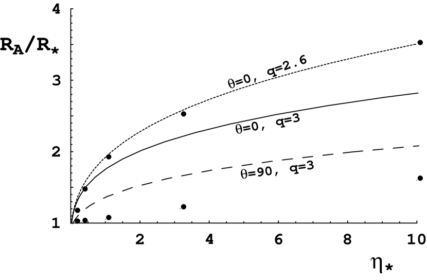
Figure 1: Variation Alfven radius $R_{A}$ with magnetic confinement parameter $\eta_{\ast}$. The points indicate MHD simulation model results above the pole (upper set) or near the magnetic equator (lower set). The lines show estimates from the magnetic field approximation of eqn. (8), applied at the equator ($\theta=90\arcdeg$; dashed line), or at the pole ($\theta=0\arcdeg$), using radial decline power index for pure dipole ($q=3$; solid line) or modified by wind radial expansion ($q=2.6$; dotted line).

Figure 1 plots solutions of this estimate of the polar ($\theta=0$; solid curve) and equatorial ($\theta=90\arcdeg$; dashed curve) Alfven radius versus the confinement parameter $\eta_{\ast}$ for various values of the magnetic exponent $q$. The circles compare the actual computed Alfven radii near the magnetic poles (filled) and equator (open) for our MHD simulations, as will be discussed further below (§§4, 5.1).

This heuristic solution for the Alfven radius can be used (cf. BM97a) to estimate the maximum radius of a closed loop. For an assumed dipole field, this loop has surface footpoints at colatitudes $\theta_{A}$ satisfying

$$\theta_{A}=\arcsin\left[\sqrt{R_{\ast}\over R_{A}(\theta=0)}\,\right]\,,$$ (9)

which thus give the latitudes $\pm|90-\theta_{A}|\arcdeg$ bounding the region of magnetic closure about the equator.

The discussion in §5.1 examines how well these heuristic scaling arguments match the results of the full MHD simulations that we now describe.

4 MHD Simulation Results

Let us now examine results of our MHD simulations for line-driven winds. Our general approach is to study the nature of the wind outflow for various assumed values of the wind magnetic confinement parameter $\eta_{\ast}$. We first confirm that, for sufficiently weak confinement, i.e., $\eta_{\ast}\leq 0.01$, the wind is essentially unaffected by the magnetic field. But for models within the range $1/10<\eta_{\ast}<10$, the field has a significant influence on the wind. For our main parameter study, the variations in $\eta_{\ast}$ are implemented solely through variations in the assumed magnetic field strength, with the stellar and wind parameters fixed at values appropriate to a typical OB supergiant, e.g. $\zeta$ Pup, as given in Table 1. Following this, we briefly (§4.4) compare flow configurations with identical confinement parameter, $\eta_{\ast}$, but obtained with different stellar and wind parameters.

4.1 Time Relaxation of Wind to a Dipole Field

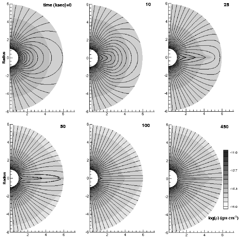
Figure 2: Snapshots of density (as logarithmic grayscale) and magnetic field (lines) at the labeled time intervals starting from the initial condition of a dipole field superposed upon a spherically symmetric outflow, for a case of mderate magnetic confinement $\eta_{\ast}=\sqrt{(}10)$ ($B_{Pole}=520G$). The intervals of field lines emanating from the star are chosen to preserve the relationship of field-line density with the strength of magnetic field.

As noted above, we study the dynamical competition between field and wind by evolving our MHD simulations from an initial condition at time $t=0$, when a dipole magnetic field is suddenly introduced into a previously relaxed, 1D spherically symmetric CAK wind. For the case of moderately strong magnetic confinement, $\eta_{\ast}=\sqrt{10}$ ($B_{o}=520$ G), figure 2 illustrates the evolution of magnetic field (lines) and density (gray scale) at fixed time snapshots, $t=$0, 10, 25, 50, 100, and 450 ksec. Note that the wind outflow quickly stretches the initial dipole field outward, opening up closed magnetic loops and eventually forcing the field in the outer wind into a nearly radial orientation. This outward field-line stretching implies a general enhancement of the magnetic field magnitude in the outer wind, as evidenced in figure 2 by the increased density of field lines at the later times. This global relaxation of field and flow is completed within the first $50-100$ ksec, corresponding to about 2-4 times the characteristic flow crossing time, $t_{flow}=5R_{\ast}/v_{\infty}\simeq 25$ ksec.

To ascertain the asymptotic behavior of flows with various magnetic confinement parameters $\eta_{\ast}$, we typically run our simulations to a time, $t=450$ ksec, that is much longer (by factor $\sim$18) than this characteristic flow time. Generally we find that, after the initial relaxation period of $\sim 50-100$ ksec, the outer wind remains in a nearly stationary configuration, with nearly steady, smooth outflow along open field lines. However, for cases with sufficiently strong magnetic field $\eta_{\ast}>1$, confinement by closed loops near the equatorial surface can lead to quite complex flows, with persistent, intrinisic variability. Before describing further this complex structure near the stellar surface, let us first examine the simpler, nearly steady flow configurations that result in the outer wind.

4.2 Global Wind Structure for Strong, Moderate, and Weak Fields

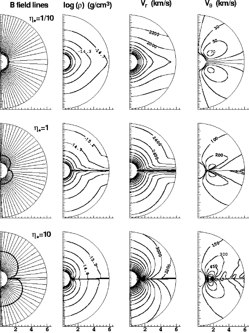
Figure 3: Comparison of overall properties at the final simulation time ($t=450$ sec) for 3 MHD models, chosen to span a range of magnetic confinement from small (top row; $\eta_{\ast}=1/10$), to medium (middle row; $\eta_{\ast}=1$), to large (bottom row; $\eta_{\ast}=10$). The leftmost panels show magnetic field lines, together with the location (bold contour) of the Alfven radius, where the radial flow speed equals the Alfven speed. From left to write, the remaining columns show contours of log(density), radial velocity, and latitudinal velocity.

Figure 3 illustrates the global configurations of magnetic field, density, and radial and latitudinal components of velocity at the final time snapshot, $t=450$ ksec after initial introduction of the dipole magnetic field. The top, middle, and bottom rows show respectively results for a weak, moderate, and strong field, characterized by confinement parameters of $\eta_{\ast}=1/10$, $1$, and $10$.

For the weak magnetic case $\eta_{\ast}=1/10$, note that the flow effectively extends the field to almost a purely radial configuration everywhere. Nonetheless, even in this case the field still has a noticeable influence, deflecting the flow slightly toward the magnetic equator (with peak latitudinal speed $\max(v_{\theta})\simeq 70$ km/s) and thereby leading to an increased density and a decreased radial flow speed in the equatorial region.

For the moderate magnetic strength $\eta_{\ast}=1$, this equatorward deflection becomes more pronounced, with a faster latitudinal velocity component ($\max(v_{\theta})\simeq 300$ km/s), and a correspondingly stronger equatorial change in density and radial flow speed. The field geometry shows moreover a substantial nonradial tilt near the equatorial surface.

For the strong magnetic case $\eta_{\ast}=10$, the near-surface fields now have a closed-loop configuration out to a substantial fraction of a stellar radius above the surface. Outside and well above the closed region, the flow is quasi-steady, though now with substantial channeling of material from higher latitudes toward the magnetic equator, with $\max(v_{\theta})>500$ km/s, even outside the closed loop. This leads to a very strong flow compression, and thus to a quite narrow equatorial “disk” of dense, slow outflow.

This flow configuration is somewhat analagous to the “Wind Compressed Disk” model developed for non-magnetic, rotating winds (Bjorkman and Cassinelli 1993; Owocki, Cranmer, and Blondin 1994). Indeed, it was already anticipated as a likely outcome of magnetic channeling, e.g. by BM97b, and in the “WC-Fields” paradigm described by Ignace, Bjorkman and Cassinell (1998). It is also quite analogous to what is found for strong field channeling in other types of stellar wind (Matt et al. 2000), including even the solar wind (Keppens and Goedbloed 1999 2000).

4.3 Variability of Near-Surface Equatorial Flow

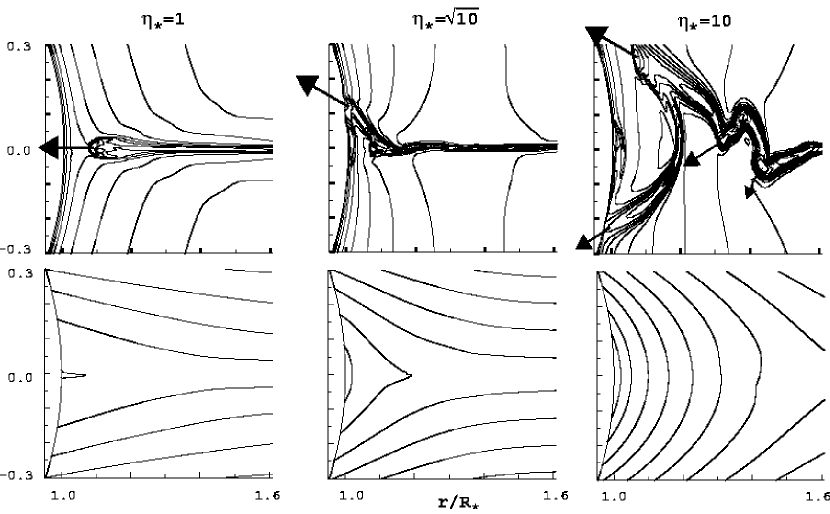
Figure 4: Contours of log(density) (upper row) and magnetic field lines (lower row) for the inner, magnetic-equator regions of MHD models with moderate ($\eta_{\ast}=1$; left), strong ($\eta_{\ast}=\sqrt{10}$; middle), and strongest ($\eta_{\ast}=10$; left) magnetic confinement, shown at a fixed, arbitary time snapshot well after ($t\geq 400$ ksec) the initial condition. The arrows represent the direction and magnitude of the mass flux, and show clearly that the densest structures are undergoing an infall back onto the stellar surface. For the moderate magnetic confinement $\eta_{\ast}=1$, this infall is directly along the equator, but for the higher confinements $\eta_{\ast}=\sqrt{10}$ and $10$, the equatorial compressions that form at larger radii are deflected randomly toward the north or south as they fall in toward the closed field near the surface. The intent here is to illustrate how increasing magnetic confinement leads to an increasing complexity of flow and density structure within closed magnetic loops. This complexity is most vividly illustrated in the time animations available in the electronic version of the paper.

In contrast to this relatively steady, smooth nature of the outer wind, the flow near the star can be quite structured and variable in the equatorial regions. For the strong magnetic field case $\eta_{\ast}=10$, the complex structure of the flow within the closed magnetic loops near the equatorial surface is already apparent even in the global contour plots in the bottom row of figure 3. To provide a clearer illustration of this variable flow structure, Figure 4 zooms in on the near-star equatorial region, comparing density (upper row, contours), mass flux (arrows), and field lines (lower row) at an arbitray time snapshot long after the initial condition at an arbitray time snapshot long after the initial condition ($t>400$ ksec), for three models with magnetic confinement numbers $\eta_{\ast}=$ 1, $\sqrt{10}$, and 10.

For the case of moderate magnetic field with $\eta_{\ast}=1$, note the appearance of the high-density knot at a height $\sim 0.3R_{\ast}$ above the equatorial surface. As is suggested from the bow-shaped front on the inward-facing side of this knot, it is flowing inward, the result of a general infall of material that had been magnetically channeled into an equatorial compression, and thereby became too dense for the radiative line-driving to maintain a net outward acceleration against the inward pull of the stellar gravity. This again is quite analogous to the inner disk infall found in dynamical simulations of rotationally induced Wind Compressed Disks (Owocki, Cranmer, and Blondin 1994).

Animations of the time evolution for this case show that such dense knots form repeatedly at semi-regular intervals of about 200 ksec. A typical cycle begins with a general building of the equatorial density through the magnetic channeling and equatorial compression of wind outflow from higher latitudes. As the radiative driving weakens with the increasing density, the equatorial outflow first decelerates and then reverses into an inflow that collects into the dense knot. Once the equatorial density is emptied by the knot falling onto the surface, the build-up begins anew, initiating a new cycle.

For the case of somewhat stronger field with $\eta_{\ast}=\sqrt{10}$, the snapshot at the same fixed time $t=400$ ksec again shows evidence for an infalling knot, except that now this has been forced by the magnetic tension of an underlying, closed, equatorial loop to slide to one hemisphere (in this case north), instead of falling directly upon the equatorial stellar surface. Animations of this case show a somewhat more irregular repetition, with knots again forming about every 200 ksec, but randomly sliding down one or the other of the footpoint legs of the closed equatorial loop. It is interesting that, even though our simulations are formally symmetric in the imposed conditions for the two hemispheres, this symmetry is spontaneously broken when material from the overlying dense equatorial flow falls onto, and eventually off of, the top of the closed magnetic loop.

The strongest field case with $\eta_{\ast}=10$ shows a much more extensive magnetic confinement, and accordingly a much more elaborate configuration for material re-accretion onto the surface. Instead of forming a single knot, the equatorially compressed material now falls back as a complex “snake” of dense structure that breaks up into a series of dense knots, draining down the magnetic loops toward both northern and southern footpoints. In the time animations for as long as we have run this case, there is no clear repetition time, as the formation and infall of knots and snake-segments are quite random, perhaps even chaotic.

It is worth noting here that in the two stronger magnetic cases, the closed loops include a region near the surface for which the field is so nearly horizontal that it apparently inhibits any net upflow. As a consequence, these loops tend to become quite low density. This has an unfortunate practical consequence for our numerical simulations, since the associated increase in the Alfven speed requires a much smaller numerical time step from the standard Courant condition. Thus far this has effectively limited our ability to run such strong field models for the very extended time interval needed for clearer definition of the statistical properties of the re-accretion process.

In contrast to this effective inhibition of radial outflow by the nearly horizontal field in the central regions of a closed loop, note that in the outer portion of the loop, where the field is more vertical, the radial line-driving is able to initiate a supersonic flow up along the loop. But when this occurs along a field line that is still closed, the inevitable result is that material from opposite footpoints is forced to collide near the top of the loop. This effectively halts the outflow for that field line, with the accumulating material near the top of the loop supported by both the magnetic tension from below and the ram pressure of incoming wind from each side.

As the density builds, maintaining this support against gravity becomes increasingly difficult. For the moderate field strength, the material from all such closed flow tubes accumulates into a knot whose weight forces the loop top to buckle inward, first nearly symmetrically but eventually off toward one side, allowing the material to re-accrete toward that footpoint at the surface. For the strongest field, the loops tend to remain nearly rigid, keeping the material from distinct closed flow tubes separate and suspended at loop tops with a range of heights, until this line of material finally breaks up into segments (the “snake”) that fall to either side of the rigid re-accretion tubes.

It is interesting to contrast this inferred outflow and re-accretion in the magnetic equator of a line-driven wind with what occurs in the solar coronal expansion. For the solar wind, acceleration to supersonic speeds typically occurs at a height of several solar radii above the surface. As such, magnetic loops that typically close within such heights can generally maintain the gas in a completely hydrostatic stratification. By contrast, in line-driven winds supersonic speeds are typically achieved very near the stellar surface, within about $0.1R_{\ast}$. A closed loop that starts from a radially oriented footpoint thus simply guides this line-driven outflow along the loop, instead of confining a hydrostatic stratification. For a strong field with sufficiently high loop top, the eventual shock collision can have velocity jumps that are a substantial fraction of the wind terminal speed, e.g. $\sim 1000$ km/s. In the present isothermal simulations, the heating from such shocks is assumed to be radiated away over a narrow, unresolved cooling layer. In the discussion in §5.3.4, we estimate some general properties of the associated X-ray emission.

Table 1: Summary Table

	Model
							$\eta_{\ast}=\sqrt{10}$
Quantity	$\eta_{\ast}=0$	$\eta_{\ast}=\frac{1}{10}$	$\eta_{\ast}=\frac{1}{\sqrt{10}}$	$\eta_{\ast}=1$	$\eta_{\ast}=\sqrt{10}$	$\eta_{\ast}=10$	low $\dot{M}$	$\theta^{1}$ Ori C
$\alpha$	0.6	0.6	0.6	0.6	0.6	0.6	0.6	0.5
$\bar{Q}$	500	500	500	500	500	500	20	700
$\delta$	0.0	0.0	0.0	0.0	0.0	0.0	0.0	0.1
$R_{\ast}(10^{12}cm)$	1.3	1.3	1.3	1.3	1.3	1.3	1.3	0.5
$B_{Pole}$(G)	0	93	165	295	520	930	165	480
$\rho_{0}$($10^{-11}gm\,cm^{-3}$)	4.3	4.3	4.3	4.3	4.3	4.3	0.54	2.8
max($v_{r})(km\;s^{-1})$	2300	2350	2470	2690	2830	3650	2950	2620
max($v_{\theta})(km\;s^{-1})$	0	70	150	300	400	1200	400	450
$\dot{M}_{net}$($10^{-6}M_{\odot}~{}yr^{-1}$)	2.6	3.0	2.8	2.5	2.2	1.8	0.22	0.3

4.4 Comparing Models with Different Stellar Parameters but Fixed $\eta_{\ast}$

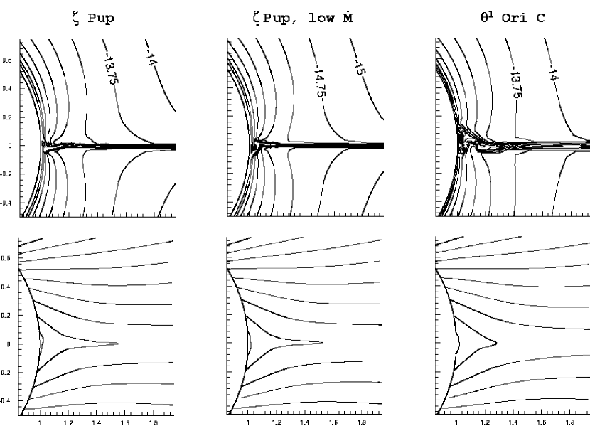
Figure 5: Contours for log of density (upper row) and magnetic fields (lower row) in the inner regions of 3 MHD models with a fixed magnetic confinement parameter $\eta_{\ast}=\sqrt{10}$, but obtained using different stellar and wind parameters, chosen to correspond to an O-type supergiant like $\zeta$ Pup with normal (left) or factor-ten lower mass loss rate (middle), or to a late-O giant like $\theta^{1}$ Ori C (right). The overall similarity of the three models illustrates the degree to which the global configuration of field and flow depends mainly on just the combination of stellar, wind, and magnetic properties that define [via eqn. (7] the magnetic confinement parameter $\eta_{\ast}$.

The models above use different magnetic field strengths to vary the magnetic confinement for a specific O supergiant star with fixed stellar and wind parameters. To complement that approach, let us briefly examine models with a fixed confinement parameter $\eta_{\ast}=\sqrt{10}$, but now manifest through different stellar and/or wind parameters. Specifically, figure 5 compares density contours (top) and field lines (bottom) for our standard $\zeta Pup$ model (center panels), with a model in which the mass loss rate is reduced by a factor 10 (left panels), and also with a model based on entirely different stellar and wind parameters, intended roughly to represent the O7 star $\theta^{1}$ Ori C (right panels). (Detailed parameter values are given in Table 1.)

Note that all three models have very similar overall form in both their density contours and field lines, even though the associated magnitudes vary substantially from case to case. This similarity of structure for models with markedly different individual parameters, but configured to give roughly equal $\eta_{\ast}$, thus further reinforces the notion that this confinement parameter is the key determinant in fixing the overall competition between field and flow.

5 Analysis and Discussion

5.1 Comparison of MHD Simulations with Heuristic Scaling Estimates

The above results lend strong support to the general idea, outlined in §3.1, that the overall effect of a magnetic field in channeling and confining the wind outflow depends largely on the single magnetic confinement parameter $\eta_{\ast}$. Let us now consider how well these MHD simulation results correspond to the heuristic estimates for the Alfven radius $R_{A}$ and magnetic closure colatitude $\theta_{A}$ defined in §3.2.

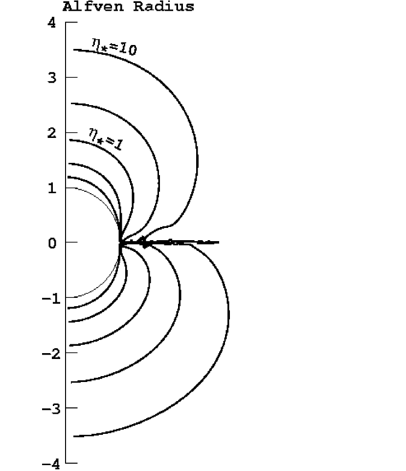
Figure 6: Contours of the Alfven radius in MHD models with confinement parameters (from inside-out) $\eta_{\ast}=$ 1/10, $1/\sqrt{10}$, 1, $\sqrt{10}$, and $10$.

Figure 6 plots contours of the Alfven radius obtained in the numerical MHD simulations with various $\eta_{\ast}$. Reflecting the stronger field and so higher Alfven speed, the models with larger confinement parameter have a higher Alfven radius. Note, moreover, that for all cases the Alfven radius generally decreases toward the equator. In part, this just reflects the Alfven speed associated with the dipole surface magnetic field, which has a lower strength near the magnetic equator.

But the comparison in figure 6 shows a systematic discrepancy between the curves showing the expected Alfven radius from this dipole model and the points showing the actual MHD results. Specifically, the dipole model underestimates the MHD Alfven radius over the pole, and overestimates it at the equator.

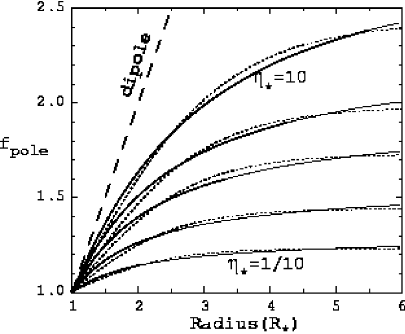
Figure 7: The measure of faster-than-$r^{2}$ decline of the polar magnetic field, as represented by the function $f_{pole}$ defined in eqn. (10), and applied to the 5 MHD simulations with magnetic confinement ranging from strong ($\eta_{\ast}=10$; uppermost curve) to weak ($\eta_{\ast}=10$; lowermost curve). For the ideal MHD cases here of field-frozen flow, this also represents the degree of faster-than-$r^{2}$ expansion of flow tube area. The dotted curves plot the heuristic area-expansion function defined by Kopp and Holzer [eqn. (11) here], with $R_{1}=1~{}R_{\ast}$, and the parameters $f_{max}=$ 2.43, 1.98, 1.73, 1.44 and 1.23, and $\sigma/R_{\ast}=$ 1.13, 0.98, 0.89, 0.79, and 0.73, chosen to best fit to the five cases from $\eta_{\ast}=$10 to 1/10. The dashed curve shows the variation for a pure dipole field.

For the polar wind, this can be understood as a consequence of the radial stretching of the field. Figure 7 plots the radial variation of the polar field ratio

$$f_{pole}(r)\equiv{R_{\ast}^{2}B_{o}\over r^{2}B(r,0)}$$ (10)

for the various magnetic confinement parameters $\eta_{\ast}$. For comparison, a dipole field (with $B\sim r^{-q}$ and $q=3$) would just give a straight line of unit slope (dashed line), whereas a pure monopole, radial field (with $q=2$) would give a horizontal line at value unity, $f_{pole}=1$.

The results show that the MHD cases are intermediate between these two limits. For the weakest confinement $\eta_{\ast}=1/10$, the curve bends toward the horizontal at quite small heights, reflecting how even the inner wind is strong enough to extend the polar field into a nearly radial orientation and divergence. For the strongest confinement $\eta_{\ast}=10$, the field divergence initially nearly follows the dashed line for a dipole ($q=3$), but then eventually also bends over as the wind ram pressure overwhelms the magnetic confinement and again stretches the field into a nearly radial divergence. The intermediate cases show appropriately intermediate trends, but in all cases it is significant that the radial decline in field strength is generally less steep than for a pure dipole, i.e. $q<3$. The dotted line in figure 1 indeed shows that the MHD results for the polar Alfven radii of the various confinement cases are in much better agreement with a simple scaling that assumes a radial decline (power index $q=2.6$) that is intermediate between the dipole ($q=3$) and monopole (i.e. radial divergence, $q=2$) limits.

Overall then, at the poles the radial stretching of field by the outflowing wind has the net effect of reducing the radial decline of field, and thus increasing the Alfven radius over the value expected from the simple dipole estimate of eqn. (8).

By contrast, at the equator this radial stretching has a somewhat opposite effect, tending to remove the predominantly horizontal components of the equatorial dipole field, and thus leading to a lower equatorial field strength and so also a lower assoicated Alfven radius, relative to the simple dipole analysis of §4.2. For example, for the lowest confinement case $\eta_{\ast}=1/10$, the field is extended into a nearly radial configuration almost right from the stellar surface, as shown by the top left panel of figure 3; the equatorial polarity switch of this radial field thus implies a vanishing equatorial Alfven speed, which thus means that contours of Alfven radius must bend sharply inward toward the surface near the equator. For the strongest confinement case $\eta_{\ast}=10$, the near-surface horizontal field within closed magnetic loops about the equator remains strong enough to resist this radial stretching by wind outflow; but the faster radial fall-off in magnetic vs. flow energy means that the field above these closed loops is eventually stretched outward into a radial configuration, thus again leading to a vanishing equatorial field and an associated inward dip in the Alfven radius.

This overall dynamical lowering of the equatorial strength of magnetic field further means that the latitudinal extents of closed loops in full MHD models are generally below what is predicted by the simple dipole estimate of eqn. (9). Thus, in previous semi-analytic models of BM97b, which effectively assume this type of dipole scaling, a somewhat larger surface field is needed to give the assumed overall extent of magnetic confinement.

5.2 Effect of Magnetic Field on Mass Flux and Flow Speed

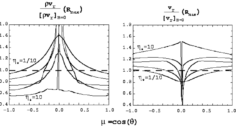
Figure 8: The radial mass flux density $\rho v_{r}$ (left) and radial flow speed $v_{r}$ (right) at the maximum model radius $R_{max}=6R_{\ast}$, normalized by values in the corresponding non-magnetic model, and plotted versus the cosine of the colatitude, $\cos(\theta)$, for the final time snaphsot ($t=450$ ksec) in the 5 MHD models with magnetic confinement parmeters $\eta_{\ast}=~{}1/10$, $1/\sqrt{10}$, 1, $\sqrt{10}$, and 10. The horizontal dashed lines mark the unit values for the non-magnetic ($B=\eta_{\ast}=0$) case.

Two key general properties of spherical, non-magnetic stellar winds are the mass loss rate ${\dot{M}}\equiv 4\pi\rho v_{r}r^{2}$ and terminal flow speed $v_{\infty}$. To illustrate how a stellar magnetic field can alter these properties for a line-driven wind, figure 8 shows the outer boundary ($r=R_{max}$) values of the radial velocity, $v_{r}(R_{max},\theta)$, and radial mass flux density, $\rho(R_{max},\theta)v_{r}(R_{max},\theta)$, normalized by the values (given in Table 1) for the non-magnetic, spherically symmetric wind case, and plotted as a function of $\mu=\cos(\theta)$ for each of our simulation models with various confinement parameters $\eta_{\ast}$.

There are several noteworthy features of these plots. Focussing first on the mass flux, note that in all models the tendency of the field to divert flow toward the magnetic equator leads to a general increase in mass flux there, with this equatorial compression becoming narrower with increasing field strength, until, for the strongest field, it forms the spike associated with an equatorial disk. This higher equatorial mass flux is associated with a higher density, since the equatorial flow speeds are always lower, quite markedly so for the dense, slowly outflowing disk of the strong field case.

Table 1 lists the overall mass loss rates, obtained by integration of these curves over the full range $-1<\mu<1$. For the strong field case, the mass loss is reduced relative to the non-magnetic ${\dot{M}}$, generally because the magnetic confinement and tilt of the inner wind outflow has effectively inhibited some of the base mass flux. Curiously, for the weakest magnetic confinement case $\eta_{\ast}=1/10$, there is actually a modest overall increase in the mass loss. The reasons for this are not apparent, and will require further investigation.

5.2.1 Role of Rapid Areal Divergence in Enhancing Wind Flow Speed

The right panel in figure 8 shows that the wind flow speed over the poles is enhanced relative to a spherical wind. This is quite reminiscent of the high-speed polar flow in the solar wind (Smith, Balogh, Forsyth, & McComas 2001; Horbury & Balogh 2001), which is generally understood to emanate from polar coronal holes of open magnetic field (Zirker 1977). Modeling of such high-speed solar wind has emphasized the important role of faster-than-radial area divergence in such open field regions (Kopp and Holzer 1976; Holzer 1977; Wang and Sheeley 1990).

Indeed, based on this solar analogy, MacGregor (1988) analyzed the effect of such rapid divergence on a line-driven stellar wind, assuming a simple 1D, radially oriented flow tube, as expected near the polar axis of an open magnetic field. He concluded that, because the line-driving acceleration scales inversely with density [$g_{lines}\sim 1/\rho^{\alpha}$; see eqn. (5)], the lower density associated with faster divergence would lead to substantially faster terminal speeds, up to a factor three faster than in a spherical wind, for quite reasonable values of the assumed flow divergence parameters. By comparison, the polar flow speed increases found in our full MHD models here are much more modest, about 30% in even the strongest field case, $\eta_{\ast}=10$.

Because field and flow lines are locked together in the ideal MHD cases assumed here, the quantity $f_{pole}$, defined in eqn. (10) and plotted in figure 7, actually also represents just this non-radial flow divergence factor for the polar flow. It is thus worthwhile to compare these dynamically computed divergence factors to the divergence assumed by MacGregor (1988), which was based on a heuristic form introduced originally by Kopp and Holzer (1976) for the solar case

$$f(r)={f_{max}\exp[(r-R_{1})/\sigma]+1-(f_{max}-1)\exp[(R_{\ast}-R_{1})/\sigma]\over\exp[(r-R_{1})/\sigma]+1}\,.$$ (11)

Specifically, these previous analyses generally assumed that the rapid divergence would be confined to a quite narrow range of radius ($\sigma=0.1R_{\ast}$) centered on some radius ($R_{1}=1.25-2.5\,R_{\ast}$) distinctly above the stellar surface radius $R_{\ast}$. By comparison, our dynamical simulations indicate the divergence is generally most-rapid right at the wind base (implying $R_{1}\approx R_{\ast}$), and extends over a quite large radial range (i.e., $\sigma>1R_{\ast}$). On the other hand, the MacGregor (1988) assumed values of the asymptoptic net divergence, $f_{max}=1.25-2.0$, are quite comparable the divergence factors found at the outer boundary of our MHD simulation models, $f_{pole}(R_{max})=1.25-2.5$.

These detailed differences in radial divergence do have some effect on the overall wind acceleration, and thus on the asymptotic flow speed. But it appears that the key reason behind the MacGregor (1988) prediction of a very strong speed enhancement was the neglect there of the finite-disk correction factor for the line-force (Friend and Abbott 1986; Pauldrach, Puls, and Kudritzki 1986). With this factor included, and using the MHD simulations to define both the divergence and radial tilt-angle of the field and flow, we find that a simple flow-tube analysis is able to explain quite well our numerical simulation results for not only the polar speed, but also for the latitudinal scaling of both the speed and mass flux. In particular, we find that the even stronger increase in flow speed seen at mid-latudes ($1/4<|\mu|<3/4$) in the strongest field model ($\eta_{\ast}=10$) does not reflect any stronger divergence factor, but rather is largely a consequence of a reduced base mass flux associated with a nonradial tilt of the source flow near the stellar surface. As the flow becomes nearly radial somewhat above the wind base, the lower density associated with the lower mass flux implies a stronger line-acceleration and thus a faster terminal speed along these mid-latitude flow tubes. Further details of these findings will be given in future paper.

5.3 Observational Implications of these MHD Simulations

5.3.1 UV Line-Profile Variability

It is worth emphasizing here that these dynamical results for the radial flow speed have potentially important implications for interpreting the observational evidence for wind structure and variability commonly seen in UV line profiles of hot stars (e.g., the so-called Discrete Absorption Components; Henrichs et al. 1994; Prinja and Howarth 1986; Howarth and Prinja 1989). In particular, an increasingly favored paradigm is that the inferred wind structure may arise from Corotating Interaction Regions (CIRs) between fast and slow speed wind streams. This requires a base perturbation mechanism to induce latitudinal variations in wind outflow properties from the underlying, rotating star (Mullan 1984; Cranmer and Owocki 1996). Based largely on the analogy with solar wind CIRs – for which the azimuthal variations in speed are clearly associated with magnetic structure of the solar corona (Zirker 1977; Pizzo 1978) –, there has been a longstanding speculation that surface magnetic fields on hot stars could similarly provide the base perturbations for CIRs in line-driven stellar winds (Mullan 1984; Shore & Brown 1990, Donati 2001).

However, until now, one argument against this magnetic model for hot-star-wind structure was the expectation, based largely on the Macgregor (1988) analysis, that a sufficiently strong field would likely lead to anomalously high-speed streams, in excess of 5000 km/s, representing the predicted factor of two or more enhancement above the speed for a non-magnetic wind (Owocki 1994; BM97a). By comparison, the wind flow speeds inferred quite directly from the blue edges of strong, saturated P-Cygni absorption troughs of UV lines observed from hot stars show only a modest variation of a few hundred km/s, with essentially no evidence for such extremely fast speeds (Prinja et al. 1998).

The full MHD results here are much more in concert with this inferred speed variation, even for the strongest field model, for which the fastest streams are not much in excess of $\sim$3000 km/s. Moreover, in conjunction with the reduced flow speeds toward the magnetic equator, there is still quite sufficient speed contrast to yield very strong CIRs, if applied in a rotating magnetic star with some substantial tilt between magnetic and rotation axes. Through extensions of the current 2D models to a full 3D configuration, we plan in the future to carry out detailed simulations of winds from rotating hot-stars with such a tilted dipole surface field, applying these specifically toward the interpretation of observed UV line profile variability.

5.3.2 Infall within Confined Loops and Red-Shifted Spectral Features

In addition to the slowly migrating discrete absorption components commonly seen in the blue absorption troughs of P-Cygni profiles of UV lines, there are also occasional occurences of redward features in either absorption (e.g., in $\tau$ Sco; Howk et al. 2000) or emission (e.g., in $\lambda$ Eri and other Be or B supergiant stars; Peters 1986; Smith, Peters, and Grady 1991; Smith 2000; Kaufer 2000). Within the usual context of circumstellar material that is either in an orbiting disk or an outflowing wind, such redshifted spectral features have been difficult to understand, since they require material flowing away from the observer, either in absorption against the stellar disk, or in emission from an excess of receding material radiating from a volume not occulted by the star. In general this thus seems to require material infall back toward the star and onto the surface. Indeed, there have been several heuristic models that have postulated such infall might result from a stagnation of the wind outflow, for example due to clumping (Howk et al. 2000), or decoupling of the driving ions (Porter and Skouza 1999).

In this context, the dynamical MHD models here seem to provide another, quite natural explanation, namely that such infall is an inevitable outcome of the trapping of wind material within close magnetic loops whenever there sufficiently strong wind magnetic confinement, $\eta_{\ast}\geq 1$. In principal, such interpretations of observed red-shifts in terms of infall within closed magnetic loops could offer the possibility of a new, indirect diagnostic of stellar magnetic properties. For example, the observed redshift speed could be associated with a minimium required loop height to achieve such a speed by gravitational infall. In future studies, we thus intend to generate synthetic line absorption and emission diagnostics for these MHD confinement models, and compare these with the above cited cases exhibiting redshifted spectral features.

5.3.3 Effect on Density-Squared Emission

In addition to such effects on spectral line profiles from scattering, absorption, or emission lines, the extensive compression of material seen in these MHD models should also lead to an overall enhancement of those types of emission, both in lines and continuum, for which the volume emission rate scales with the square of the density. Specific examples include line emission from both collisional excitation or recombination, or free-free continuum emission in the infrared and radio. In principle, the former might even lead to a net emission above the continuum in the hydrogen Balmer lines, and thus to formal classification as a Be star, even without the usual association of an orbiting circumstellar disk. Such a mechanism may in fact be the origin for the occasional occurence of hydrogen line emission in slowly rotating B stars, most notably $\beta$ Ceph, for which there has indeed now been a positive detection of a tilted dipole field of polar magnetic around 300 G (Donati et al. 2001; Henrichs et al. 2000). Again, further work will be needed to apply the dynamical MHD models here toward interpretation of observations of density-square emissions from hot stars that seem likely candidates for substantial wind magnetic confinement.

5.3.4 Implications for X-ray Emission

Particularly noteworthly among the potential observational consequences of these MHD models are the clear implications for interpreting the detection of sometimes quite hard, and even cyclically variable, X-ray emission from some hot stars. As noted in the introduction, there have already been quite extensive efforts to model such X-ray emission within the context of a fixed magnetic field that channels wind flow into strong shock collisions (BM97a,b). In contrast, while the isothermal MHD models here do not yet include the detailed energy balance treatment necessary for quantitative modeling of such shocked-gas X-ray emission, they do provide a much more complete and dynamically consistent picture of the field and flow configuration associated with such magnetic channeling and shock compression.

Indeed, as a prelude to future quantitative models with explicit computations of the energy balance and X-ray emission, let us briefly apply here an approximate analysis of our model results that can yield rough estimates for the expected level of compressional heating and associated X-ray production. The central idea is to assume that, within the context of the present isothermal models, any compressive heating that occurs is quickly balanced by radiative losses within a narrow, unresolved cooling layer (Castor 1987; Feldmeier et al. 1997; Cooper 1994). For shock-type compressions with a sufficiently strong velocity jump, this radiative emission should include a substantial component in the X-ray bandpass.

Applying this perspective, we first identify within our simulation models locations of locally strong compressions, i.e. where there are substantial zone to zone decreases in flow speed along the direction of the flow itself. Taking into account that the quadratic viscosity within the Zeus code typically spreads any shocks over about 3 or 4 zones, we can use this to estimate an associated total shock jump in the specific kinetic energy $\Delta v^{2}/2$. We then apply the standard shock jump conditions to obtain a correponding estimate of post-shock temperatures (BM97b),

$$T_{s}\approx 2.7\times 10^{5}\,K~{}{-\Delta v^{2}/2\over(100\,km/s)^{2}}\,.$$ (12)

Figure 9c shows contours of $T_{s}$ computed in this way for the strong confinement case $\eta_{\ast}=10$. Note that quite high temperatures, in excess of $10^{7}$ K, occur in both closed loops near the surface, as well as for the open-field, equatorial disk outflow in the outer wind. For the closed loops, where the field forces material into particularly strong, nearly head-on, shock collisions, this is as expected from previous fixed-field models (BM97a,b).

But for the open-field, equatorial disk outflow, the high-temperature compression is quite unexpected. Since the flow impingent onto the disk has a quite oblique angle, dissipation of just the normal component of velocity would not give a very strong shock compression. But this point of view assumes a “free-slip” post-shock flow, i.e., that the fast radial flow speed would remain unchanged by the shock. However, our simulations show that the radial speed within the disk is much slower. Thus, under the more realistic assumption that incoming material becomes fully entrained with the disk material, i.e. follows instead a “no-slip” condition, then the reduction from the fast radial wind speed implies a strong dissipation of radial flow kinetic energy, and thus a quite high post-shock temperature.

To estimate the associated magnitude of expected X-ray emission, we first compute the local volume rate of compressive heating, obtained from the negative divergence of the local kinetic energy flux,

$$q\equiv-\nabla\cdot({\bf v}\rho v^{2}/2)\approx-\rho{\bf v}\cdot\nabla v^{2}/2\,.$$ (13)

The contours of $q$ plotted in figure 9d again show that strong compressions are concentrated toward the magnetic equator, with again substantial levels occuring in both the inner, closed loops, as well as in the equatorial disk outflow.

Let us next combine these results to estimate the X-ray emission above some minimum threshold energy $E$, weighting the emission by a “Boltzmann factor” that declines exponentially with the ratio of this energy to the shock energy $kT_{s}$,

$$q_{E}\equiv q\,e^{-E/kT_{s}}\,.$$ (14)

Using the conversion that a soft X-ray energy threshold of $E=0.1$ keV corresponds roughly to a temperature of $1.1\times 10^{6}$ K, the contours in figure 9e show that soft X-rays above this energy would again be produced in both the inner and outer regions of the equatorial disk.

Figures 9 d and e show that the volume for flow compression and associated X-ray emission is quite limited, confined to narrow disk about the magnetic equator. Nonetheless, the strength of this emission can be quite significant. For example, volume integration of the regions defined in figure 9d give a total rate of energy compression $L_{c}\sim 10^{36}$ erg/s, which represents about 25% of the total wind kinetic energy, $L_{w}\sim{\dot{M}}v_{\infty}^{2}/2\sim 4\times 10^{36}$ erg/s.

This is consistent with the fraction of mass loss in the slowly outflowing, equatorial disk, which has a value ${\dot{M}_{eq}}\sim 5\times 10^{-7}~{}M_{\odot}$/yr, or about the same 25% of the total wind mass loss rate ${\dot{M}}\sim 2\times 10^{-6}\,M_{\odot}$/yr. The terminal speed within this disk, $v_{eq}\sim$ 1000 km/s, is about a third of that in the wind, $v_{\infty}\sim$ 3000 km/s, implying nearly an order magnitude lower specific kinetic energy. The ‘missing’ energy associated with this slow disk outflow thus represents roughly the total wind flow kinetic energy dissipated by the flow into this slow disk.

Finally, integration of the Boltzmann-weighted emission in figure 9e gives an estimate for the soft X-ray emission above 0.1 keV of $L_{x}\sim 10^{35}$ erg/s. This is substantially higher than the canonical X-ray emission associated with intrinsic wind instabilities, $L_{x}\sim 10^{-7}L_{bol}\sim 4\times 10^{32}$ erg/s. This supports the general notion that hot-stars with anomalously large, observed X-ray luminosities might indeed be explained by flow compressions associated with wind-magnetic channeling.

While this analysis thus provides a rough estimate of the X-ray emission properties expected from such MHD models of wind magnetic confinement, we again emphasize that quantitative calculations of expected X-ray emission levels and spectra will require a future, explicit treatment of the wind energy balance.

6 Result Summary

We have carried out 2D MHD simulations of the effect of stellar dipole magnetic fields on radiatively driven stellar winds. The initial simulations here are based on idealizations of isothermal flow driven outward from a non-rotating star by a strictly radial line-force. The principal results are summarized as follows:

1. The general effect of magnetic field in channeling the stellar wind depends on the overall ratio of magnetic to flow-kinetic-energy density, as characterized by the wind magnetic confinement parameter, $\eta_{\ast}$, defined here in eqn. (7). For typical stellar and wind parameters of hot, luminous supergiants like $\zeta$ Pup, moderate confinement with $\eta_{\ast}\sim 1$ requires magnetic fields of order 100 Gauss. The results of standard, spherically symmetric, non-magnetic wind models are recovered in the limit of very small magnetic confinement, $\eta_{\ast}\leq 0.01$.

2. For moderately small confinement, $\eta_{\ast}=1/10$, the wind extends the surface magnetic field into an open, nearly radial configuration. But even at this level, the field still has a noticeable global influence on the wind, enhancing the density and decreasing the flow speed near the magnetic equator.

3. For intermediate confinement, $\eta_{\ast}=1$, the fields are still opened by the wind outflow, but near the surface retain a signifcant non-radial tilt, channeling the flow toward the magnetic equator with a latitudinal velocity component as high as 300 km/s.

4. For strong confinement, $\eta_{\ast}=10$, the field remains closed in loops near the equatorial surface. Wind outflows accelerated upward from opposite polarity footpoints are channeled near the loop tops into strong collision, with characteristic shock velocity jumps of up to about 1000 km/s, strong enough to lead to hard ($>~{}1$ keV) X-ray emission.

5. Even for strong surface fields, the more rapid radial decline of magnetic vs. wind-kinetic-energy density means the field eventually becomes dominated by the flow, and extended into an open configuration.

6. The compression of open-field outflow into a dense, slowly outflowing equatorial disk can lead to shocks that are strong enough to produce quite hard X-ray emission, a possibility that was completely unaccounted for in previous fixed-field analyses that focussed only on X-ray emission within closed loops (BM97a,b).

7. In contrast to these previous steady-state, fixed-field models, the time-dependent dynamical models here indicate that stellar gravity pulls the compressed, stagnated material within closed loops into an infall back onto the stellar surface, often through quite complex, intrinsically variable flows that follow magnetic channels randomly toward either the north or south loop footpoint.

8. Compared with expectations of previous semi-analytic, heuristic analyses, the dynamical simulations here show some distinct differences in the overall properties of field and flow, for example with a narrower region of equatorial confinement, and an Alfven radius that is lower at the pole and higher at the equator.

9. The outflows from magnetic poles show quite gradual non-radial area expansions, with terminal wind speeds enhanced by factors (generally $\leq$1.3) that are much less than the factor three increase predicted by previous 1D flow-tube analyses (MacGregor et al. 1988). The more modest level of wind velocity modulation seen in full MHD simulations here is much more compatible with observed blue-edges of absorption troughs in UV wind lines from hot stars.

10. Finally, these MHD simulations have many properties relevant to interpreting various kinds of observational signatures of wind variability and structure, e.g. UV line discrete absorption components; red-shifted absorption or emission features; enhanced density-square emission; and X-ray emission.

In the future, we plan to extend our simulations to include non-radial line-forces, an explicit energy balance with X-ray emission, and stellar rotation. We then intend to apply these simulations toward quantitive modeling of the various observational signatures of wind structure that might be associated with magnetic fields in hot stars.

Acknowledgements. This research was supported in part by NASA grant NAG5-3530 and NSF grant AST-0097983 to the Bartol Research Institute at the University of Delaware. A. ud-Doula acknowledges support of NASA’s Space Grant College program at the University of Delaware. We thank D. Cohen, C. deKoning, and V. Dwarkadas for helpful discussions and comments.

References

- Abbott (1982) Abbott, D. C. 1982, ApJ, 259, 282
- Babcock (1960) Babcock, H. W. 1960, ApJ, 132, 521
- Babel & Montmerle (1997a) Babel, J. & Montmerle, T. 1997, A&A, 323, 121
- Babel & Montmerle (1997b) Babel, J. & Montmerle, T. 1997, ApJ, 485,L29
- Bjorkman & Cassinelli (1993) Bjorkman, J. E. & Cassinelli, J. P. 1993, ApJ, 409, 429
- Bohlender, Landstreet, & Thompson (1993) Bohlender, D. A., Landstreet, J. D., & Thompson, I. B. 1993, A&A, 269, 355
- Borra & Landstreet (1980) Borra, E. F. & Landstreet, J. D. 1980, ApJS, 42, 421
- Cassinelli & MacGregor (2000) Cassinelli, J. P. & MacGregor, K. B. 2000, ASP Conf. Ser. 214: The Be Phenomenon in Early-Type Stars, 337
- Castor (1987) Castor, J. I. 1987, ASSL Vol. 136: Instabilities in Luminous Early Type Stars, 159
- Castor, Abbott, & Klein (1975) Castor, J. I., Abbott, D. C., & Klein, R. I. 1975, ApJ, 195, 157
- Charbonneau & Macgregor (2001) Charbonneau, P. & MacGregor, K. B. 2001, ApJ, 559, 1094.
- Cooper (1994) Cooper, R. G. 1994, Ph.D. Thesis, 22
- Courant & Hilbert (1953) Courant, R. & Hilbert, D. 1953, New York: Interscience Publication, 1953,
- Cranmer & Owocki (1996) Cranmer, S. R. & Owocki, S. P. 1996, ApJ, 462, 469
- Donati et al. (2001) Donati, J.-F., Wade, G. A., Babel, J., Henrichs, H. F., de Jong, J. A., Harries, T. J. 2001, MNRAS, 326, 1265
- Drew (1989) Drew, J. E. 1989, ApJS, 71, 267
- Feldmeier (1995) Feldmeier, A. 1995, A&A, 299, 523
- Feldmeier et al. (1997) Feldmeier, A., Kudritzki, R.-P., Palsa, R., Pauldrach, A. W. A., & Puls, J. 1997, A&A, 320, 899
- Friend & Abbott (1986) Friend, D. B. & Abbott, D. C. 1986, ApJ, 311, 701
- Gayley (1995) Gayley, K. G. 1995, ApJ, 454, 410
- Gayley & Owocki (2000) Gayley, K. G. & Owocki, S. P. 2000, ApJ, 537, 461
- Henrichs et al. (2000) Henrichs, H. F. et al. 2000, Magnetic Fields of Chemically Peculiar and Related Stars, Proceedings of the International Meeting, held in Special Astrophysical Observatory of Russian AS, September 23 - 27, 1999, Eds.: Yu.V. Glagolevskij, I.I. Romanyuk, p.57-60, 57
- Henrichs, Kaper, & Nichols (1994) Henrichs, H. F., Kaper, L., & Nichols, J. S. 1994, A&A, 285, 565
- Holzer (1977) Holzer, T. E. 1977, J. Geophys. Res., 82, 23
- Horbury & Balogh (2001) Horbury, T. S. & Balogh, A. 2001, J. Geophys. Res., 106, 115929
- Howarth & Prinja (1989) Howarth, I. D. & Prinja, R. K. 1989, ApJS, 69, 527
- Howarth & Smith (1995) Howarth, I. D. & Smith, K. C. 1995, ApJ, 439, 431
- Howk, Cassinelli, Bjorkman, & Lamers (2000) Howk, J. C., Cassinelli, J. P., Bjorkman, J. E., & Lamers, H. J. G. L. M. 2000, ApJ, 534, 348
- Ignace, Cassinelli, & Bjorkman (1998) Ignace, R., Cassinelli, J. P., & Bjorkman, J. E. 1998, ApJ, 505, 910
- Ignace, Cassinelli, & Nordsieck (1999) Ignace, R., Cassinelli, J. P., & Nordsieck, K. H. 1999, ApJ, 520, 335
- Ignace, Nordsieck, & Cassinelli (1997) Ignace, R., Nordsieck, K. H., & Cassinelli, J. P. 1997, ApJ, 486, 550
- Kaper et al. (1996) Kaper, L., Henrichs, H. F., Nichols, J. S., Snoek, L. C., Volten, H., & Zwarthoed, G. A. A. 1996, A&AS, 116, 257
- Kaufer (2000) Kaufer, A. 2000, ASP Conf. Ser. 214: The Be Phenomenon in Early-Type Stars, 37
- Keppens & Goedbloed (1999) Keppens, R. & Goedbloed, J. P. 1999, A&A, 343, 251
- Keppens & Goedbloed (2000) Keppens, R. & Goedbloed, J. P. 2000, ApJ, 530, 1036
- Kopp & Holzer (1976) Kopp, R. A. & Holzer, T. E. 1976, Sol. Phys., 49, 43
- Long & White (1980) Long, K. S. & White, R. L. 1980, ApJ, 239, L65
- Lucy (1982) Lucy, L. B. 1982, ApJ, 255, 286
- MacGregor (1988) MacGregor, K. B. 1988, ApJ, 327, 794
- Mathias et al. (2001) Mathias, P., Aerts, C., Briquet, M., De Cat, P., Cuypers, J., Van Winckel, H., Flanders., & Le Contel, J. M. 2001, A&A, 379, 905
- Mathys (1995) Mathys, G. 1995, A&A, 293, 746
- Mathys et al. (1997) Mathys, G., Hubrig, S., Landstreet, J. D., Lanz, T., & Manfroid, J. 1997, A&AS, 123, 353
- Matt, Balick, Winglee, & Goodson (2000) Matt, S., Balick, B., Winglee, R., & Goodson, A. 2000, ApJ, 545, 965
- Mullan (1984) Mullan, D. J. 1984, ApJ, 283, 303
- Owocki (1994) Owocki, S. P. 1994, Ap&SS, 221, 3
- Owocki, Castor, & Rybicki (1988) Owocki, S. P., Castor, J. I., & Rybicki, G. B. 1988, ApJ, 335, 914
- Owocki, Cranmer, & Blondin (1994) Owocki, S. P., Cranmer, S. R., & Blondin, J. M. 1994, ApJ, 424, 887
- Owocki, Cranmer, & Gayley (1996) Owocki, S. P., Cranmer, S. R., & Gayley, K. G. 1996, ApJ, 472, L115
- Pauldrach (1987) Pauldrach, A. 1987, A&A, 183, 295
- Pauldrach, Puls, & Kudritzki (1986) Pauldrach, A., Puls, J., & Kudritzki, R. P. 1986, A&A, 164, 86
- Peters (1986) Peters, G. J. 1986, ApJ, 301, L61
- Pizzo (1978) Pizzo, V. 1978, J. Geophys. Res., 83, 5563
- Pneuman & Kopp (1971) Pneuman, G. W. & Kopp, R. A. 1971, Sol. Phys., 18, 258
- Porter & Skouza (1999) Porter, J. M. & Skouza, B. A. 1999, A&A, 344, 205
- Priest & Hood (1991) Priest, E.R.,Hood, A.W. 1991, Advances in Solar System Magnetohydrodynamics, Cambridge: Cambridge University Press, 1991
- Prinja & Howarth (1986) Prinja, R. K. & Howarth, I. D. 1986, ApJS, 61, 357
- Prinja et al. (1998) Prinja, R. K. , Massa, D., Howarth, I. D., & Fullerton, A. W. 1998, MNRAS, 301, 926.
- Shore & Brown (1990) Shore, S. N. & Brown, D. N. 1990, ApJ, 365, 665
- Smith (2000) Smith, M. A. 2000, ASP Conf. Ser. 214: The Be Phenomenon in Early-Type Stars, 292
- Smith, Balogh, Forsyth, & McComas (2001) Smith, E. J., Balogh, A., Forsyth, R. J., & McComas, D. J. 2001, Geophys. Res. Lett., 28, 4159
- Smith, Peters, & Grady (1991) Smith, M. A., Peters, G. J., & Grady, C. A. 1991, ApJ, 367, 302
- Sobolev (1960) Sobolev, V. V. 1960, Soviet Astronomy, 4, 372
- Stone & Norman (1992) Stone, J. M. & Norman, M. L. 1992, ApJS, 80, 753
- Telting, Aerts, & Mathias (1997) Telting, J. H., Aerts, C., & Mathias, P. 1997, A&A, 322, 493
- van Leer (1977) van Leer, B. 1977, Journal of Computational Physics, 23, 276
- Wang & Sheeley (1990) Wang, Y.-M. & Sheeley, N. R. 1990, ApJ, 355, 726
- Zirker (1977) Zirker, J. B. 1977, Coronal Holes and High Speed Wind Streams, Boulder: Colorado Associated University Press.