Cosmological Recombination of Lithium and its Effect on the Microwave Background Anisotropies

Abstract

The cosmological recombination history of lithium, produced during Big–Bang nucleosynthesis, is presented using updated chemistry and cosmological parameters consistent with recent cosmic microwave background (CMB) measurements. For the popular set of cosmological parameters, about a fifth of the lithium ions recombine into neutral atoms by a redshift $z\sim 400$. The neutral lithium atoms scatter resonantly the CMB at 6708 Å  and distort its intensity and polarization anisotropies at observed wavelengths around $\sim 300~{}\mu$m, as originally suggested by Loeb (2001). The modified anistropies resulting from the lithium recombination history are calculated for a variety of cosmological models and found to result primarily in a suppression of the power spectrum amplitude. Significant modification of the power spectrum occurs for models which assume a large primordial abundance of lithium. While detection of the lithium signal might prove difficult, if offers the possibility of inferring the lithium primordial abundance and is the only probe proposed to date of the large-scale structure of the Universe for $z\sim 500-100$.

1 Introduction

Lithium is the heaviest stable element produced during Big–Bang nucleosynthesis (Burles, Nollett, & Turner, 2001, and references therein). However, due to its low primordial abundance relative to hydrogen $X_{\rm Li}\sim 10^{-10}$–$10^{-9}$, its significance in the early Universe was thought to be restricted only to the formation of rare molecules such as LiH (Stancil, Lepp, & Dalgarno, 1996, and references therein). Hence, the recombination history of lithium itself was only calculated as an intermediate step in a chain of chemical reactions and under a set of simplifying assumptions (Palla, Galli, & Silk, 1995; Stancil, Lepp, & Dalgarno, 1996, 1998, hereafter SLD96, SLD98). These preliminary calculations indicated that a substantial fraction ($\gtrsim 20$%) of the singly-charged lithium ions formed neutral atoms by recombination in the redshift interval $z\sim 400$–$500$.

Recently, Loeb (2001) has shown that the formation of neutral lithium can strongly modify the anisotropy maps of the cosmic microwave background (CMB) through the absorption and re-emission at its resonant 6708 Å transition from the ground state. Despite the exceedingly low lithium abundance left over from the Big Bang, the resonant optical depth after lithium recombination is expected to be as high as $\tau_{{}_{\rm LiI}}\sim 0.4(X_{\rm Li}/3.8\times 10^{-10})$ at a redshift $z\sim 400$ if half of the lithium ions recombine by then. The scattering refers to an observed wavelength of $\lambda(z)=[6708~{}$Å$\times(1+z)]=268.3~{}\mu{\rm m}\times[(1+z)/400]$, where $X_{{}_{\rm Li}}\approx 3.8\times 10^{-10}$ is the latest estimate of the lithium to hydrogen number density ratio (Burles et al., 2001). Loeb (2001) argued that resonant scattering would suppress the original anisotropies by a factor of $\exp({-\tau_{{}_{\rm LiI}}})$, but will generate new anisotropies in the CMB temperature and polarization on sub–degree scales primarily through the Doppler effect. Observations at different far–infrared wavelengths could then probe different thin slices of the early Universe. Zaldarriaga & Loeb (2002) calculated in detail the expected anisotropies in both the temperature and polarization of the CMB and assessed their detectability relative to the far-infrared background. They concluded that the modified polarization signal could be comparable to the expected polarization anisotropies of the far-infrared background on sub-degree angular scales ($\ell\gtrsim 100$). However, these calculations assumed a range of trial values for the neutral fraction of lithium in the redshift range $z=400$–500 lacking knowledge of its full redshift dependence.

In this paper, we calculate rigorously the recombination history of lithium and its subsequent effect on the CMB anistoropies. In §2 we discuss the physics responsible for the recombination history of lithium and in §3 we obtain the resulting optical depth for the 6708 Å transition. §4 describes the effects of the lithium optical depth on the CMB power spectra. Finally, §5 summarizes this work.

2 The Lithium Recombination History

In order to assess the importance of the optical depth of lithium on the CMB anisotropies, an accurate determination of the neutral lithium abundance as a function of redshift is required. The post–recombination abundance of Li was first addressed by Lepp & Shull (1984) in their investigation of molecules formed in the early Universe. While this work gave no information on the Li and Li⁺ abundances or the adopted rate coefficients, they were implicitly needed to obtain the LiH abundance, a main focus of their study. Puy et al. (1993) also investigated the LiH post-recombination abundance, but neglected to give any details concerning the evolution of Li and Li⁺.

The first explicit results for the redshift dependent Li and Li⁺ abundances were presented by Palla et al. (1995) although no information was given on the adopted chemistry or reaction rate coefficients. Their results, which varied little with the adopted cosmological model parameters, suggested that the neutral Li formation redshift was $z_{\rm f}\sim 500$ (which we define here as the redshift when the neutral abundance reaches 10% of the elemental abundance $n_{\rm Li}$) and that the Li ionization fraction $n$(Li⁺)/$n_{\rm Li}\to 0.16$ as $z\to 0$. The significant residual Li⁺ abundance, a result predicted by Dalgarno & Lepp (1987), is a consequence of the depletion of electrons following the cosmological recombination of hydrogen and helium. The related chemistry was described in more detail and improved upon in SLD96, Bougleux & Galli (1997), and Galli & Palla (1998, hereafter GP98). The primary Li formation and destruction mechanisms are radiative recombination

$${\rm Li}^{+}+{\rm e}^{-}\rightarrow{\rm Li}+\nu,$$ (1)

(L5) and photoionization,

$${\rm Li}+\nu\rightarrow{\rm Li}^{+}+{\rm e}^{-},$$ (2)

(L10) respectively. For the former, they adopted the rate coefficients of Verner & Ferland (1996, VF96) which is based on R-matrix calculations of the photoionization cross sections of Li (Peach, Saraph, & Seaton, 1988), but adjusted to match experiment, and smoothly fit to higher-energy Hartree-Dirac-Slater calculations (Verner et al., 1996). Through comparison of their photoionization cross sections to experiment, VF96 suggest that their Case A recombination coefficients are accurate to better than 10%. The Li photoionization rate for a black-body radiation field was then obtained by detailed balance from the radiative recombination rate coefficients (see GP98). Using the same cosmological models of Palla et al. (1995) (see also Model III of SLD96), Bougleux & Galli (1997) found similar results, $z_{\rm f}\sim 500$ and $n$(Li⁺)/$n_{\rm Li}=0.18$ at $z=10$. However, with further improvements in the chemistry, GP98 predicted $z_{\rm f}\sim 400$ and $n$(Li⁺)/$n_{\rm Li}=0.56$ at $z=10$.

In their comprehensive chemistry SLD96 adopted the radiative recombination coefficients of Caves & Dalgarno (1972) determined from their model potential calculations of the photoionization cross sections. SLD96 also estimated the photoionization rate by detailed balance and found $z_{\rm f}\sim 450$ and $n$(Li⁺)/$n_{\rm Li}=0.34$ at $z=10$ (using the same cosmological parameters, Model III). Following improvements in the lithium chemistry (see Stancil & Dalgarno, 1997, 1998; Stancil & Zygelman, 1996), SLD98 obtained $z_{\rm f}\sim 440$ and $n$(Li⁺)/$n_{\rm Li}=0.48$ at $z=10$. Figure 1 displays the lithium abundances as a function of redshift from various calculations using Model III of SLD96.

To explore the dependencies of the models on the adopted rate coefficients, we repeated the calculations of SLD98, but using the rate coefficients for reactions (1) and (2) from GP98. The small changes shown in Figure 1 reflect the fact that the radiative recombination rate coefficients of VF96 are only about 5% larger than those determined by Caves & Dalgarno (1972), which is however within the 10% accuracy claimed by VF96. Any differences in the rate coefficients of other processes result in only secondary effects as can be seen in Figure 2 which displays both the formation and destruction rates (multiplied by the neutral Li fractional abundance $n({\rm Li})/n_{\rm H}$) of the dominant processes and their time scales (per Hubble time $1/H(z)$). For $z>500$, the CMB field at temperatures $T>1300$ K efficiently photoionizes any neutral Li atom produced, but at lower redshifts the photoionization rate (reaction 2, L10) falls precipitously, allowing the rapid increase in neutral Li through reaction (1, L5). Figure 2 shows clearly that for $z<500$, the only important process is radiative recombination (1, L5) with the radiative charge transfer reaction

$${\rm Li}+{\rm H}^{+}\rightarrow{\rm Li}^{+}+{\rm H}+\nu$$ (3)

(L13, Stancil & Zygelman, 1996) being only marginally significant with a rate about two orders of magnitude smaller. Further, neutral Li is mostly made over the narrow redshift interval $z\sim 500-300$, before its formation time-scale becomes greater than the Hubble time.

While the minor differences in the rate coefficients are unable to explain the discrepancies between the Li and Li⁺ abundances of GP98 and SLP98, it seems likely that the adopted hydrogen recombination model may be responsible for the difference. For $z<650$, GP98 obtained a smaller electron fractional abundunce $x_{\rm e}$, with the SLD98 result being $\sim 60\%$ larger by $z=100$. This trend is in agreement with the lithium abundances displayed in Figure 1 indicating a significant dependence on electron abundance, as would be expected. Given that the two hydrogen recombination models are rather rudimentary, it would seem appropriate to use an improved model. An ameliorated hydrogen recombination calculation has been performed by Seager, Sasselov, & Scott (2000) (see also Seager et al., 1999) which allowed for the H excited state populations to depart from equilibrium. Their calculation which consists of a 300-level model H atom including all relevant bound-bound and bound-free transitions, finds a change for the electron fraction of about 10% from simple equilibrium population results. Seager et al. (1999) have provided the program RECFAST which emulates their detailed nonequilibrium population calculation. We have coupled RECFAST to our code and obtained the lithium abundances shown in Figure 1 where we have also continued to use the GP98 rate coefficients for reactions (1) and (2), and for the remainder of this work. The neutral Li abundance has increased further as the electron abundance computed by RECFAST is larger than obtained from both GP98 and SLD98, being about 80% larger than GP98 at $z=100$. Henceforth, the electron abundances will be obtained from RECFAST.

The cosmological parameters (Model III of SLD96) used above have been superseded by new values based on analysis of the latest CMB anisotropy experiments (e.g., de Bernardis et al., 2002; Jaffe et al., 2001; Wang, Tegmark, & Zaldarriaga, 2001). To explore the range of possible Li abundances allowable within the CMB uncertainties, we considered the five models listed in Table 1. Model A is considered our fiducial case as all parameters are consistent with the best fit values of Wang et al. (2001, the third column of their Table 2). Model B has the same values, but uses $h=0.75$, close to $h=0.72$ from the HST Hubble Key Project (Freedman et al., 2001). Models A and B are also consistent with the BOOMERANG experiment (de Bernardis et al., 2002). Models C and D follow the result of Jaffe et al. (2001), $\Omega_{\rm b}h^{2}=0.032_{-0.004}^{+0.005}$, which is also just barely outside of the 95% confidence limit of Wang et al. (2001, see their Table 5). Model E is an extreme case taken as the upper limit from Jaffe et al. (2001). The corresponding primordial abundances ($Y$, $X_{\rm D}$, and $X_{\rm Li}$) were obtained from Burles et al. (2001).

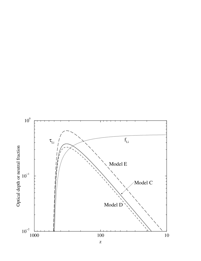
Figure 4: The lithium neutral fraction and optical depth for Models C ($h=0.65$, $\Omega_{b}h^{2}=0.03$), D ($h=0.75$, $\Omega_{b}h^{2}=0.03$), and E ($h=0.65$, $\Omega_{b}h^{2}=0.037$).

Using the electron abundances determined with RECFAST, the latest lithium chemistry model of SLD98 with some improvements listed in Lepp, Stancil, & Dalgarno (2002), but with the rate coefficients for reactions (1, L5) and (2, L10) replaced by the values from GP98, and the parameters listed in Table 1, we have calculated the new lithium neutral fractions shown in Figures 3 and 4. The neutral lithium fraction is defined as

$$f_{\rm Li}(z)={{n({\rm Li})}\over{n_{\rm Li}}}={{n({\rm Li})}\over{n({\rm Li})+n({\rm Li^{+}})}},$$ (4)

where

$$n({\rm Li})=f_{\rm Li}(z)X_{\rm Li}n_{\rm H}(z)$$ (5)

and

$$n_{\rm H}(z)=1.123\times 10^{-5}(1-Y)\Omega_{\rm b}h^{2}(1+z)^{3}~{}{\rm cm}^{-3}.$$ (6)

The lithium neutral fractions $f_{\rm Li}$ are identical for Models A and B and for Models C and D, while comparison of all the models reveal very little differences. In fact, for all models $z_{\rm f}\sim 440$ and $f_{\rm Li}=0.55-0.56$ (or $n$(Li⁺)/$n_{\rm Li}=0.44-0.45$) at $z=10$.

3 The Optical Depth of Neutral Lithium

The Sobolev optical depth of neutral lithium is given by

$$\tau_{\rm Li}(z)=\sum_{u}{{\lambda_{1u}^{3}A_{u1}}\over{8\pi}}{{g_{u}}\over{g_{1}}}{{n({\rm Li})(1-b)}\over{H(z)}},$$ (7)

(see Seager et al., 2000; Bougleux & Galli, 1997, equation A9) where

$$H(z)^{2}=H_{0}^{2}\biggl{[}{{\Omega_{0}}\over{1+z_{\rm eq}}}(1+z)^{4}+\Omega_{0}(1+z)^{3}+\Omega_{\rm K}(1+z)^{2}+\Omega_{\Lambda}\biggr{]},$$ (8)

$b$ accounts for the fraction of neutral Li in excited states, $g_{u}$ and $g_{1}$ are the degeneracies of the upper and ground states, respectively, and the sum is over the excited $2p~{}^{2}P_{J}$ fine-structure levels $J=1/2,3/2$. We took $b=0$ and adopted the wavelengths 6707.76 and 6707.91 Å  for the $1/2\to 3/2$ and $1/2\to 1/2$ transitions from the NIST Atomic Spectra Database (1999) which also gives the transition probability $A_{21}=3.72\times 10^{7}$ s^-1 for both transitions. The optical depths for Models A-E are plotted in Figures 3 and 4. In all cases, $\tau_{\rm Li}$ is maximum near $z\sim 325$ where $f_{\rm Li}\sim 0.275$. Over the five models, the maximum $\tau_{\rm Li}$ varies from $\sim 0.1$ to $\sim 0.66$ which can be compared to the redshift independent optical depths of 0.5–2 adopted by Zaldarriaga & Loeb (2002). Only the extreme Model E approaches the optical depths considered by Zaldarriaga & Loeb (2002). As expected (see Loeb, 2001; Zaldarriaga & Loeb, 2002), the optical depth increases with $X_{\rm Li}$, but the current results also demonstrate that $\tau_{\rm Li}$ increases with $\Omega_{\rm b}h^{2}$ and decreases with $h$.

Making the approximation $H(z)=\Omega_{0}^{1/2}H_{0}(1+z)^{3/2}$ and taking Model A as the fiducial case, we find that the optical depth reduces to

$$\tau_{\rm Li}(z)=0.380f_{\rm Li}(z)\biggl{(}{{X_{\rm Li}}\over{3.907\times 10^{-10}}}\biggr{)}\biggl{(}{{1-Y}\over{0.75286}}\biggr{)}\biggl{(}{{\Omega_{\rm b}h^{2}}\over{0.02}}\biggr{)}\biggl{(}{{0.65}\over{h}}\biggr{)}\biggl{(}{{0.33}\over{\Omega_{0}}}\biggr{)}^{1/2}\biggl{(}{{1+z}\over{300}}\biggr{)}^{3/2},$$ (9)

which can be compared to equation (1) of Zaldarriaga & Loeb (2002). The numerical trends discussed above are evident in this relation in addition to dependencies on $Y$ and $\Omega_{0}$. The shape of the optical depth curves arise from a competition between the increasing neutral Li fraction $f_{\rm Li}$ and the expansion of the Universe. As a consequence, the possible effects of lithium on the CMB power spectrum are restricted to the epoch of $z\sim 100-500$.

4 Effects on CMB Anisotropies

We have calculated the signatures of lithium resonant scattering on the CMB anisotropies following the methods described in Zaldarriaga & Loeb (2002). To isolate the effect of the scatterings we have kept all cosmological parameters fixed as we varied the optical depth. As a reference model we considered the standard LCDM model and compared it with models having optical depths equal to those of models A, C and E of the previous section.

In Figure 5 we show the temperature anisotropy power spectra predicted for a wavelength of $\lambda=268.3~{}\mu m$ (corresponding to scattering at a redshift $z=400$). In Figure 6 we show the analogous plot for polarization. The effect of the scatterings increases as the optical depth increases, so they are the smallest in model A and the largest in model E. The changes are dominated by two contributions: (i) the Doppler anisotropies induced at the sharp lithium scattering surface and (ii) the uniform $\exp(-\tau_{\rm Li})$ suppression of the primary anisotropies which were generated at decoupling.

At large multipoles $l$ (small angular scales), Figure 6 illustrates how the $\exp(-\tau_{\rm Li})$ suppression of the anisotropies reduces the amplitude of power spectra by a factor $\exp(-2\tau_{{\rm Li}})$. This effect leaves the shape of the power spectra unchanged. For the models under consideration the optical depth ranges from $0.1$ to $0.6$ so on these scales the power spectra are suppressed by a factor between $0.3$ and $0.8$.

As was discussed by Zaldarriaga & Loeb (2002), the Doppler effect reaches a maximum on degree scales and is responsible for the change of shape of the power spectra on these scales. This effect can be noticed most dramatically in model E for the temperature and in both models C and E for the polarization.

Measurements of the CMB anisotropies at long photon wavelengths such as those that will be made by the MAP and Planck satellites, will provide a baseline for comparison against which the effect of lithium could be extracted. These long wavelength maps, which are unaffected by the lithium scattering, can be compared with maps obtained at shorter wavelengths. In particular a useful statistic to study is the power spectra of the difference map (see Zaldarriaga & Loeb 2001 for details). Here we subtract the power spectra obtained at long wavelengths from that observed at 268.3 $\mu$m, and consider the power spectrum of the residuals. The results for this statistic are presented in Figure 7.

Figure 7 indicates that the largest signal relative to the unperturbed spectra is expected in polarization at degree angular scales $(l\sim 200)$. In this range and for both models C and E, the power in the difference spectrum is comparable to (or even larger than) the power in the long wavelength spectrum.

Table 1: Cosmological model parameters.

Parameter	Model A	Model B	Model C	Model D	Model E
$\Omega_{0}$	0.33	0.33	0.33	0.33	0.33
$\Omega_{\rm K}$	0.0	0.0	0.0	0.0	0.0
$\Omega_{\Lambda}$	0.67	0.67	0.67	0.67	0.67
$z_{\rm eq}$	1.01e4	1.35e4	1.01e4	1.35e4	1.01e4
$\Omega_{\rm b}h^{2}$	0.02	0.02	0.03	0.03	0.037
$\eta_{10}$	5.479	5.479	8.219	8.219	10.14
$\Omega_{\rm b}$	4.734e-2	3.556e-2	7.101e-2	5.333e-2	8.757e-2
$h$	0.65	0.75	0.65	0.75	0.65
$Y$	0.24714	0.24714	0.25108	0.25108	0.25298
$X_{\rm D}$	3.105e-5	3.105e-5	1.611e-5	1.611e-5	1.116e-5
$X_{\rm Li}$	3.907e-10	3.907e-10	8.560e-10	8.560e-10	1.197e-9

5 Discussion

We have calculated the recombination history of lithium for a set of different cosmological parameters (see Table 1). The resulting opacity to the 6708 Å  resonant transition of neutral lithium (Figs. 3 and 4) distorts both the temperature (Fig. 5) and polarization (Fig. 6) power-spectra of the CMB anisotropies over a band of observed photon wavelengths around $\sim 300~{}\mu$m. The distortion is most pronounced in model E which assumes a relatively high lithium abundance of $X_{\rm Li}=1.2\times 10^{-9}$. Our detailed results agree with earlier estimates by Loeb (2001) and Zaldarriaga & Loeb (2001). The predicted polarization signal is comparable to the expected polarization anisotropies of the far-infrared background (FIB; see Zaldarriaga & Loeb 2001). A strategy for eliminating the contribution from the brightest FIB sources would be helpful in isolating the lithium signal.

The relevant wavelength range overlaps with the highest frequency channel of the Planck mission ($352~{}\mu$m), with the Balloon–borne Large–Aperture Sub–millimeter Telescope (BLAST) that will have $250,\ 350$ and $500~{}\mu$m channels and with the proposed balloon–borne Explorer of Diffuse Galactic Emissions (EDGE) that will survey 1% of the sky in 10 wavelength bands between $230$–$2000~{}\mu$m with a resolution ranging from $6^{\prime}$ to $14^{\prime}$ (see Table 1 in Knox et al. 2001). However, in order to optimize the detection of the lithium signature on the CMB anisotropies, a new instrument design is required with multiple narrow bands ($\Delta\lambda/\lambda\lesssim 0.1$) at various wavelengths in the range $\lambda=250$–$350~{}\mu$m. The experiment should cover a sufficiently large area of the sky so as to determine reliably the statistics of fluctuations on degree scales, and the detector should be sensitive to polarization. For reference, the experiment should also measure the anisotropies at shorter wavelengths where the FIB dominates. All of these requirements, of course, will make the detection of the lithium signature a difficult experiment. The difficulty cannot be fully accessed until more is known about the FIB and the sources responsible for it. Some considerations and strategies are discussed in Zaldarriaga & Loeb (2002). Further, in order to detect the effect of lithium, high signal-to-noise maps of the primordial CMB at long wavelengths should be made for the same region of the sky. Fortunately, these maps will become available from future CMB missions such as the Planck satellite.

On the theoretical front, improvements on the predicted lithium recombination history can be made by performing an explicit calculation of the non-equilibrium populations of the excited states in the same level-by-level fashion as that of the hydrogen recombination calculation of Seager et al. (1999, 2000). For hydrogen it was found that the excited state levels were overpopulated for $z<800$ as the levels fall-out of equilibrium with the background radiation field. A slower photoionization rate coupled with faster cascade rates results in a faster net recombination rate ultimately resulting in a $\sim$10% change in the ionization fraction. Seager et al. (1999, 2000) also confirmed that all Lyman transitions are optically thick during hydrogen recombination indicating that Case B recombination holds at $z>800$ but not at lower redshifts. The optical depths computed here for lithium are less than one for the ground state transition suggesting that all other transitions should be optically thin, indicating Case A recombination. The Case A lithium equilibrium recombination rate coefficient of VF96 might result in an underestimation of the neutral lithium fraction (and the optical depth), but probably only by $\sim 10\%$.

We also note that non-conventional recombination histories may have a substantial impact on our predicted signal. For example, it has recently been proposed that recombination could have been delayed by the presence of additional radiation at $z\sim 10^{3}$, possibly from stars, AGNs, or accretion by primordial compact objects (Peebles, Seager, & Hu, 2000; Miller & Ostriker, 2001). The neutral fraction of lithium (and its optical depth) could be larger than we calculated based on the standard recombination history, as the neutral lithium fraction is sensitive to the residual electron abundance. However, the stronger radiation field might override any gains in recombination of lithium due to the increase in its photoionization rate. Models with detailed radiation fields are needed to calculate the net effect that these processes have on the lithium optical depth.

Finally, while experiments to observe the lithium distortion on the temperature and polarization CMB power spectra appear to require redesign of detectors and new observational strategies, the benefits as mentioned in Zaldarriaga & Loeb (2002) could potentially be significiant:

1. If the lithium signal could be separated from the FIB contamination, it would offer the possibility of constraining the lithium primordial abundance. Inferring the lithium primordial abundance from stellar observations is known to be complicated by stellar lithium depletion and galactic lithium production. Further, the lithium primordial abundance is a sensitive indicator of the baryon abundance, its mean value as well as inhomogenities. It would then provide a possible means to discriminate among Big–Bang nucleosynthesis models.

2. The lithium signature on the CMB anisotropies is the only probe proposed so far for structure in the dark ages of the early Universe. Other methods, such as the suggestion by Iliev et al. (2002) that angular fluctuations in 21 cm emission from minihalos could probe redshifts between reionization and $z\sim 20$, rely on the existence of collapsed objects and do not reach the high redshifts ($z\sim$100 to $\lesssim 500$) probed by the lithium signal (see review by Barkana & Loeb 2001). The lithium and 21 cm signals would both give measures of the baryonic density fluctuations, the latter during the era of early star formation leading to reionization and the former just before the condensation of the first objects.

Figure 1: Comparsion of various calculations of the Li and Li⁺ fractional abundance (relative to hydrogen) for the cosmological Model III of SLD96 ($\Omega_{0}=1$, $\Omega_{\rm b}=0.0367$, $h=0.67$, $\Omega_{\rm b}h^{2}=0.0165$, $Y=0.242$, and $X_{\rm Li}=2.3\times 10^{-10}$).

Figure 2: Dominant formation (solid lines) and destruction (dashed lines) processes for neutral lithium for Model III of SLD96. Panel (a) shows the rates (multiplied by the neutral Li fractional abundance $n({\rm Li})/n_{\rm H}$) and (b) shows the time scale per Hubble time $1/H(z)$ per Li atom. The reaction labels (L$x$) correspond to the process $x$ listed in SLD96.

Figure 3: The lithium neutral fraction and optical depth for Models A ($h=0.65$) and B ($h=0.75$). $\Omega_{b}h^{2}=0.02$ in both cases.

Figure 5: Temperature power-spectra of the CMB anisotropies in models with optical depths equal to those of models A, C, and E together the spectra of the standard LCDM model without lithium scattering. The figure corresponds to an observed wavelength of $268.3~{}\mu$m.

Figure 6: Polarization power-spectra of the CMB anisotropies for models with optical depths equal to those of models A, C, and E, at an observed wavelength of $268.3~{}\mu$m compared to the standard LCDM without lithium scattering.

Figure 7: Difference between a long wavelength power spectrum (such as the one that will be produced by the MAP or Planck satellites) and a power spectra at 268.3 $\mu$m when the optical depths are those of models A, C, and E. We also show the spectra for the standard LCDM model without lithium scattering. The top panel shows the results for the temperature anisotropies and the bottom one for the polarization anisotropies of the CMB.

References

- Barkana & Loeb (2001) Barkana, R. & Loeb, A. 2001, Phys. Rep., 349, 125
- Bougleux & Galli (1997) Bougleux, E. & Galli, D. 1997, MNRAS, 288, 638
- Burles et al. (2001) Burles, S., Nollett, K. M., & Turner, M. S. 2001, ApJ, 552, L1
- Caves & Dalgarno (1972) Caves, T. C. & Dalgarno, A. 1972, J. Quant. Spectrosc. Radiat. Transfer, 12, 1539
- Dalgarno & Lepp (1987) Dalgarno, A. & Lepp, S. 1987, in Astrochemistry, ed. S. P. Tarafdar & M. P. Varshni (Dordrecht: Reidel), 109
- de Bernardis et al. (2002) de Bernardis, P. et al. 2002, ApJ, 564, 559
- Freedman et al. (2001) Freedman, W. L. et al. 2001, ApJ, 553, 47
- Galli & Palla (1998) Galli, D. & Palla, F. 1998, A&A, 335, 403
- Iliev et al. (2002) Iliev, I. T., Shapiro, P. R., Ferrara, A., & Martel, H. 2002, ApJ, 572, L123
- Jaffe et al. (2001) Jaffe, A. H. et al. 2001, Phys. Rev. Lett., 86, 3475
- Knox et al. (2001) Knox, L., Cooray, A., Eisenstein, D., & Haiman, Z. 2001, ApJ, 550, 7
- Lepp & Shull (1984) Lepp, S. & Shull, J. M. 1984, ApJ, 280, 465
- Lepp et al. (2002) Lepp, S., Stancil, P. C., & Dalgarno, A. 2002, J. Phys. B, 35, R57
- Loeb (2001) Loeb, A. 2001, ApJ, 555, L1
- Miller & Ostriker (2001) Miller, M. C. & Ostriker, E. C. 2001, ApJ, 561, 496
- NIST Atomic Spectra Database (1999) NIST Atomic Spectra Database 1999, http://aeldata.phy.nist.gov/cgi-bin/AtData/main_asd)
- Palla et al. (1995) Palla, F., Galli, D., & Silk, J. 1995, ApJ, 451, 44
- Peach et al. (1988) Peach, G., Saraph, H. E, & Seaton, M. J. 1988, J. Phys. B, 21, 3669
- Peebles et al. (2000) Peebles, P. J. E., Seager, S., & Hu, W. 2000, ApJ, 539, L1
- Puy et al. (1993) Puy, D., Alecian, G., Le Bourlot, J., Léorat, J., & Pineau des Forêts, G. 1993, A&A, 267, 337
- Seager et al. (1999) Seager, S., Sasselov, D. D., & Scott, D. 1999, ApJ, 523, L1
- Seager et al. (2000) ——. 2000, ApJS, 128, 407
- Stancil & Dalgarno (1997) Stancil, P. C. & Dalgarno, A. 1997, ApJ, 490, 76
- Stancil & Dalgarno (1998) ——. 1998, Faraday Dis., 109, 61
- Stancil et al. (1996) Stancil, P. C., Lepp, S., & Dalgarno, A. 1996, ApJ, 458, 401
- Stancil et al. (1998) ——. 1998, ApJ, 509, 1
- Stancil & Zygelman (1996) Stancil, P. C. & Zygelman, B. 1996, ApJ, 472, 102
- Verner & Ferland (1996) Verner, D. A. & Ferland, G. J. 1996, ApJS, 103, 467
- Verner et al. (1996) Verner, D. A., Ferland, G. J., Korista, K. T., & Yakovlev, D. G. 1996, ApJ, 465, 487
- Wang et al. (2001) Wang, X., Tegmark, M., & Zaldarriaga, M. 2001, astro-ph/0105091
- Zaldarriaga & Loeb (2002) Zaldarriaga, M., & Loeb, A. 2002, ApJ, 564, 52