MHD Turbulence in Star-Forming Regions
and the Interstellar Medium

Abstract

MHD turbulence plays a central role in the physics of star-forming molecular clouds and the interstellar medium. MHD turbulence in molecular clouds must be driven to account for the observed supersonic motions in the clouds, as even strongly magnetized turbulence decays quickly. Driven MHD turbulence can globally support gravitationally unstable regions, but local collapse inevitably occurs. Differences in the strength of driving and the gas density may explain the very different rates of star formation observed in different galaxies. Two types of comparisons to observations are reviewed. First, the use of wavelet transform methods suggest that the driving comes from scales larger than observed molecular clouds. Second, comparison of simulated spectral cubes from models to real observations suggests that Larson’s mass-size relationship is an observational artifact. The driving mechanism for the turbulence is likely a combination of field supernovae in star-forming sections of galactic disks, and magnetorotational instabilities in outer disks and low surface brightness galaxies. Supernova-driven turbulence has a broad range of pressures with a roughly log-normal distribution. High-pressure, cold regions can be formed even in the absence of self-gravity.

1 Introduction

One of the big questions in star formation is what determines the rate of star formation in galaxies? Another, more pointed way of phrasing this question is to ask why the star formation rate in normal galaxies is so low, and why it varies so strongly, over orders of magnitude from low surface brightness galaxies, through normal galaxies, to starburst galaxies. The free-fall time for gas at typical interstellar densities is

$$t_{\rm ff}=\sqrt{\frac{3\pi}{32G\bar{\rho}}}\approx(3.4\times 10^{7}\mbox{ yr})\left(\frac{n}{1\mbox{ cm}^{-3}}\right)^{-1/2},$$ (1)

where $\bar{\rho}$ is the mean mass density of the gas, $G$ the gravitational constant and $n=\bar{\rho}/\mu$ the number density, with $\mu=2.36m_{H}$. Yet galactic ages range up to $10^{10}$ yr, and star formation continues today. What has delayed star formation sufficiently to allow it to continue?

In what might be called the standard theory of star formation, magnetic fields are invoked to answer both of these questions. If fields are strong enough, they can magnetostatically support clouds against collapse. The star formation rate would then be determined by the rate of ambipolar drift of neutral gas past ions tied to the magnetic field towards the centers of self-gravitating cores m77 ; s77 . Furthermore, if the fields are strong enough that the Alfvén speed $v_{A}$ reaches the rms velocity $v$, then strong shocks will be converted to MHD waves. As linear Alfvén waves are lossless, it was thought that motions remaining from the initial formation of the clouds might be enough to explain the observation of strongly supersonic motions in molecular clouds am75 . In this review I will explain why both of these ideas now appear questionable.

2 Decaying Turbulence

First let us consider the decay of supersonic turbulence as shown in Figure 1.

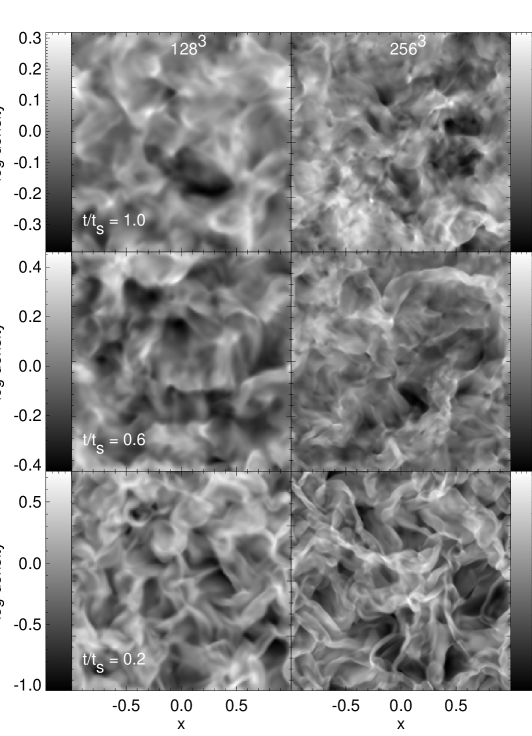
Figure 1: Log of density is shown at times $t/t_{s}=0.2$, 0.6 and 1.0 on slices through the decaying supersonic hydrodynamic models C and D with initial rms Mach number $M=5$ described in m98 at standard resolution ($128^{3}$) and high resolution ($256^{3}$), where $t_{s}$ is the sound crossing time of our numerical box. Note that each image is scaled to its own maximum and minimum to enhance morphological features (From m99 )

I call on computations performed with two different methods: Eulerian hydrodynamics and MHD on a grid, using the code ZEUS-3D sn92a ; sn92b ; c94 ; hs95 , available from the Laboratory for Computational Astrophysics at

http://zeus.ncsa.uiuc.edu/lca_home_page.html,

and Lagrangian hydrodynamics using a smoothed particle hydrodynamics (SPH) code derived from that described by Benz b90 and Monaghan m92 , running on special purpose GRAPE processors e93 ; s96 , and incorporating sink particles bbp95 .

We chose initial conditions for our models inspired by the popular idea that setting up velocity perturbations with an initial power spectrum $P(k)\propto k^{\alpha}$ in Fourier space similar to that of developed turbulence would be in some way equivalent to starting with developed turbulence pn99 ; ppw92 ; ppw94 . Observing the development of our models, it became clear to us that the loss of phase information in the power spectrum af85 allows extremely different gas distributions to have the same power spectrum. This is particularly important for supersonic flows. Supersonic, HD turbulence has been found in simulations ppw94 to have a power spectrum $\alpha=-2$. However, any single, discontinuous shock wave will also have such a power spectrum, as that is simply the Fourier transform of a step function, and taking the Fourier transform of many shocks will not change this power law. Nevertheless, most distributions with $\alpha=-2$ do not contain shocks.

After experimentation, we decided that the quickest way to generate fully developed turbulence was with perturbations having a flat power spectrum $\alpha=0$ for $0<k_{d}<8$. We set up velocity perturbutions drawn from a Gaussian random field fully determined by its power spectrum in Fourier space following the standard procedure: for each wavenumber ${\bf k_{d}}$ we randomly select an amplitude from a Gaussian distribution centered on zero and with width $P(k_{d})=P_{\rm 0}k_{d}^{\alpha}$ with $k_{d}=|{\bf k_{d}}|$, and a phase between zero and $2\pi$. We then transform the field back into real space to obtain the velocity in each zone. This is done independently for each velocity component. For the SPH calculation the velocities defined on the grid are assigned onto individual particles using the “cloud-in-cell” scheme he88 . In all of our models we take $c_{\rm s}=0.1$, initial density $\rho_{\rm 0}=1$, and we use a periodic grid with sides $L=2$ centered on the origin. These parameter choices define our unit system. Our choice of periodic boundary conditions corresponds to the case of free turbulence discussed above, at least initially. Thereafter, the appropriate treatment is less clear.

We next performed resolution studies using ZEUS for three different cases with no field, weak field and strong field as shown in Fig. 2.

Figure 2: Three-dimensional resolution studies for initial rms Mach number $M=5$, isothermal models. ZEUS models have $32^{3}$ (dotted), $64^{3}$ (short dashed), $128^{3}$ (long dashed), or $256^{3}$ (solid) zones, while the SPH models have 7000 (dotted), 50,000 (short dashed), or 350,000 (solid) particles. Panels show a) hydro runs with ZEUS, b) hydro runs with SPH, c) initial rms Alfvén number $A=v/v_{A}=5$ MHD runs with ZEUS, and d) $A=1$ MHD runs with ZEUS (From m98 )

The weak field models have an initial ratio of thermal to magnetic pressure $\beta=2$, while the strong field models have $\beta=0.08$. We ran the same unmagnetized model with the SPH code to demonstrate that our results are truly independent of the details of the viscous dissipation, and so that our lack of an explicit viscosity does not affect our results.

The kinetic energy decay curves for the four resolution studies are shown in Fig. 2. For each of our runs we performed a least-squares fit to the slope of the power-law portion of the kinetic energy decay curves. These results appear converged at the 5–10% level; it is very reassuring that the different numerical methods converge to the same result for the unmagnetized case.

We find that highly compressible, isothermal turbulence decays close to linearly in time, with $\eta=0.98$. Adding magnetic fields decreases the decay rate only slightly to $\eta\sim$0.85–0.9, with very slight dependence on the field strength or adiabatic index. Similar results have been reported by Stone, Ostriker, & Gammie sog98 and Padoan & Nordlund pn99 for compressible MHD turbulence, and by Biskamp & Müller bm00 for incompressible MHD turbulence.

The clear astrophysical implication of these models is that even strong magnetic fields, with the field in equipartition with the kinetic energy, cannot prevent the decay of turbulent motions on dynamical timescales. If molecular clouds live for longer than their dynamical time of roughly a megayear, as is generally believed even by those arguing for lifetimes under 10 Myr bhv99 ; hbb01 rather than the more classical 30 Myr bs80 , then the significant kinetic energy observed in their gas must be supplied more or less continuously.

3 Driven Turbulence

To compute the energy dissipation from uniformly driven turbulence we initialize the turbulent flow with a narrow band of $k$ values, using a top-hat function with roughly the same behavior as the steeply peaked curve used by Stone et al. sog98 in most of their models. We set the velocity field up as described above m98 . To drive the turbulence, we then normalize this fixed pattern to produce a set of perturbations $\delta\vec{\nu}(x,y,z)$, and at every time step add a velocity field $\delta\vec{v}(x,y,z)=A\delta\vec{\nu}$ to the velocity $\vec{v}$, with the amplitude $A$ now chosen to maintain constant kinetic energy input rate $\dot{E}_{\rm in}=\Delta E/\Delta t$. For compressible flow with a time-dependent density distribution, maintaining a constant energy input rate requires solving a quadratic equation in the amplitude $A$ at each time step. For a grid with $N$ zones on a side, each of volume $\Delta V$, the equation for $A$ is

$$\Delta E=\frac{1}{2}\Delta V\sum_{i,j,k=1}^{N}\rho_{ijk}A\delta\vec{\nu}_{ijk}\cdot(\vec{v}_{ijk}+A\delta\vec{\nu}_{ijk}).$$ (2)

We take the larger root of this equation to get the value of $A$. The resulting flow is shown in Fig. 3.

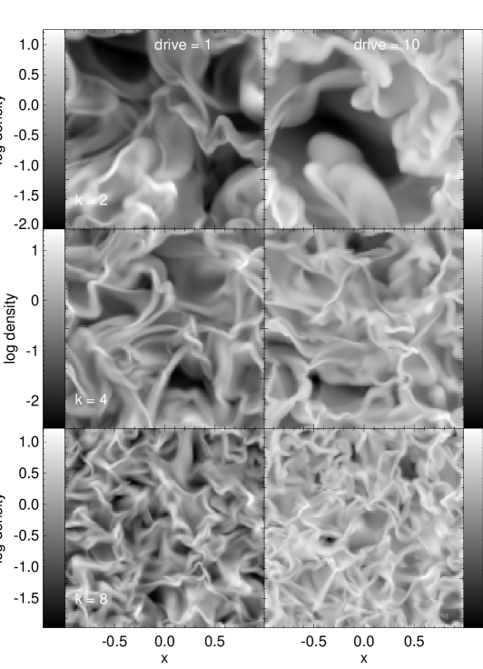
Figure 3: Models showing the appearance of turbulence with different characteristic size scales and driving energy input. Log of density on slices through hydrodynamic models from m99 at a resolution of $128^{3}$ grid points. The value of “drive” given in the figure is the driving energy input rate $\dot{E}_{\rm in}$ for that model, while $k=L/\lambda_{d}$ is the wavenumber of the driving pattern, and the size of the cube $L=2$ for all runs

We find that the best description of these compressible models comes by taking a length scale ${\cal L}=\lambda_{d}$ the driving wavelength, and a velocity scale ${\cal V}=v_{\rm rms}$ the rms velocity, rather than any of the other options available. Happily, these are just the length and velocity scales that would be expected from the theory of incompressible turbulence. Figure 4 shows

Figure 4: Energy dissipation rate for hydro and MHD models compared to $k_{d}v_{\rm rms}^{3}$ where $k_{d}$ is the dimensionless driving wavenumber, and the size of the cube $L=2$ for all runs. The lines have slope of unity, and are fit to the hydro models, yielding the value for the dissipation coefficient $\eta_{v}=0.21/\pi$ (see equation [3]). Hydrodynamical models are indicated by squares, MHD models by triangles (From m99 )

equilibrium energy dissipation rates for all the models described by Mac Low m99 , compared to the quantity $k_{d}v_{\rm rms}^{3}\sim v_{\rm rms}^{3}/\lambda_{d}$. A fit to the hydrodynamic models gives a relation with slope 1.02. Let us define a dimensionalized wavenumber $\tilde{k}=(2\pi/L)k_{d}=2\pi/\lambda_{d}$. A very good approximation is then the linear relation

$$\dot{E}_{\rm kin}\simeq-\eta_{v}m\tilde{k}v_{\rm rms}^{3},$$ (3)

with $\eta_{v}=0.21/\pi$, where the assumption is made that in equilibrium $\dot{E}_{\rm kin}=\dot{E}_{\rm in}$. The dependence on the mass of the cube $m$ comes strictly from dimensional arguments, as all of the runs shown have the same mass $m=\rho_{0}L^{3}=8$. The referee of this review points out that $\eta_{v}k_{d}\simeq 0.42\lambda_{d}^{-1}$, remarkably close to the value of $1/(2\lambda_{d})$ that would be expected by direct application of the theory of incompressible turbulence. This implies that the density variations average out almost independently of velocity variations.

The MHD models that fit equations (3) most closely are the strong field cases, with $v_{A}/c_{s}=10$. The weak field cases appear to follow a relation similar to equation (3), but with values of $\eta_{v}$ up to a factor of two higher, as shown in Figure 5.

Figure 5: Dependence of the dissipation coefficient $\eta_{v}=\dot{E}_{\rm kin}/(\tilde{k}mv_{\rm rms}^{3})$ on the plasma $\beta$, the ratio of thermal to magnetic pressure. The dashed line shows the value derived from unmagnetized models. Models with weaker fields appear to have as much as a factor two higher dissipation rate, while strong field models approach the unmagnetized rate (From m99 )

Without further computation, it remains unclear how much of the variation seen among the models with the same $\beta$ is due to random fluctuations or the remaining lack of numerical convergence, and how much is real. The higher dissipation seen in the high-$\beta$, weak-field cases could be explained by noting that weak fields will be more strongly influenced by the flow, generating more dissipative MHD waves.

We can use these results to discuss whether decaying turbulence can delay gravitational collapse. This can formally be examined by determining whether the ratio

$$\tau=t_{d}/t_{\rm ff}>1,$$ (4)

where the turbulent decay time $t_{d}=E_{\rm kin}/\dot{E}_{\rm kin}$, and the free-fall time $t_{\rm ff}$ for the gas is given by equation (1). Because $t_{d}$ depends not only on the strength of the turbulence, but also on the driving wavelength, the value of $\tau$ also depends on the ratio

$$\kappa=\lambda_{d}/\lambda_{J},$$ (5)

where the Jeans wavelength $\lambda_{J}=c_{s}\sqrt{\pi/G\rho_{0}}$. Numerical models that I disucss in the next section show that turbulence cannot support the gas against collapse at wavelengths longer than the driving wavelength lpp90 ; khm00 , so that $\kappa\leq 1$ is necessary for the turbulence to fully support against collapse.

Substituting for the values in equation (4), we can write

$$\tau=\frac{E_{\rm kin}}{\dot{E}_{\rm kin}}\frac{c_{s}}{\lambda_{J}}\sqrt{\frac{32}{3}}.$$ (6)

We can now use equation (3) for $\dot{E}_{\rm kin}$, and, somewhat less accurately, take $E_{\rm kin}\sim mv^{2}_{\rm rms}/2$, noting that this introduces no more than a 20–30% error. Substituting and using the definition of $\kappa$ given in equation (5), I find that the dissipation time scaled in units of the free fall time is

$$\tau(\kappa)=\frac{1}{4\pi\eta_{v}}\left(\frac{32}{3}\right)^{1/2}\frac{\kappa}{M_{\rm rms}}\simeq\,3.9\,\frac{\kappa}{M_{\rm rms}},$$ (7)

where $M_{\rm rms}=v_{\rm rms}/c_{s}$ is the rms Mach number of the turbulence. In molecular clouds, $M_{\rm rms}$ is typically observed to be of order 10 or higher, while $\kappa<1$ is required for support, so turbulence will decay long before the cloud collapses and not markedly influence its collapse.

4 Self-Gravitating Turbulence

Now that it is clear that driven turbulence must be present in molecular clouds, we can ask whether it alone is sufficient to support clouds against gravitational collapse.

The virial theorem provides a first way of examining this question. In equilibrium the total kinetic energy in the system adds up to half its potential energy, $E_{\rm kin}+1/2\,E_{\rm pot}=0$. If $E_{\rm kin}+1/2\,E_{\rm pot}<0$ the system collapses, while $E_{\rm kin}+1/2\,E_{\rm pot}>0$ implies expansion. In turbulent clouds, the total kinetic energy includes not only the internal energy but also the contributions from turbulent gas motions. If this is taken into account, simple energy considerations can already provide a qualitative description of the collapse behavior of turbulent self-gravitating media b87 .

A more thorough investigation, however, requires a linear stability analysis. For the case of an isothermal, infinite, homogeneous, self-gravitating medium at rest (i.e. without turbulent motions) Jeans j02 derived a relation between the oscillation frequency $\omega$ and the wave number $k$ of small perturbations,

$$\omega^{2}-c_{\rm s}^{2}k^{2}+4\pi G\,\rho_{0}=0\;,$$ (8)

where $c_{\rm s}$ is the isothermal sound speed, $G$ the gravitational constant, and $\rho_{0}$ the initial mass density. Note that the derivation includes the ad hoc assumption that the linearized version of the Poisson equation describes only the relation between the perturbed potential and the perturbed density, neglecting the potential of the homogeneous solution. This is the so-called ‘Jeans swindle’. Perturbations are unstable against gravitational contraction if their wave number is below a critical value, the Jeans wave number $k_{\rm J}$, i.e. if

$$k^{2}<k_{\rm J}^{2}\equiv\frac{4\pi G\rho_{0}}{c_{\rm s}^{2}}\;,$$ (9)

or equivalently if the wave length of the perturbation exceeds a critical size given by $\lambda_{\rm J}\equiv 2\pi k_{\rm J}^{-1}$. This directly translates into a mass limit. All perturbations with masses exceeding the Jeans mass,

$$M_{\rm J}\equiv\rho_{0}\lambda^{3}=\left(\frac{\pi}{G}\right)^{3/2}\rho_{0}^{-1/2}{c_{\rm s}^{3}},$$ (10)

will collapse under their own weight.

These and subsequent analytical approaches (reviewed in khm00 ) make a strong assumption that substantially limits their reliability, namely that the equilibrium state is homogeneous, with constant density $\rho_{0}$. However, observations clearly show that molecular clouds are extremely non-uniform. One way to achieve progress and circumvent the restrictions of a purely analytical approach is to perform numerical simulations. Bonazzola et al. b87 , for example, used low resolution ($32\times 32$ collocation points) calculations with a 2-dimensional spectral code to support their analytical results. Also restricted to two dimensions were the hydrodynamical studies by Passot et al. ppw88 , Léorat, Passot & Pouquet lpp90 , Vázquez-Semadeni et al. vpp95 and Ballesteros-Paredes, Vázquez-Semadeni & Scalo bvs99 , although performed with far higher resolution. Magnetic fields were introduced in two dimensions by Passot, Vázquez-Semadeni, & Pouquet pvp95 , and extended to three dimensions with self-gravity (though at only $64^{3}$ resolution) by Vázquez-Semadeni, Passot, & Pouquet vpp96 . A careful analysis of 1-dimensional computations including both MHD and self-gravity was presented by Gammie & Ostriker go96 , who extended their work to 2.5 dimensions more recently ogs99 .

We use ZEUS-3D and SPH to examine the gravitational stability of three-dimensional hydrodynamical turbulence at higher resolution than before, and include magnetic fields using ZEUS-3D. The use of both Lagrangian and Eulerian numerical methods to solve the equations of self-gravitating hydrodynamics in three dimensions (3D) allows us to attempt to bracket reality by taking advantage of the strengths of each approach. This also gives us some protection against interpreting numerical artifacts as physical effects.

SPH can resolve very high density contrasts because it increases the particle concentration, and thus the effective spatial resolution, in regions of high density, making it well suited for computing collapse problems as shown in Fig. 6.

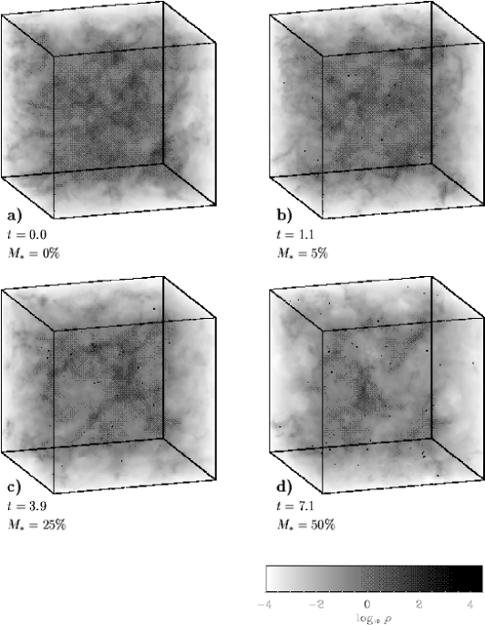
Figure 6: SPH density cubes for model driven in the wavenumber interval $3\leq k_{d}\leq 4$, shown (a) at the time when gravity is turned on, (b) when the first dense cores are formed and have accreted $M_{*}=5$% of the mass, (c) when the mass in dense cores is $M_{*}=25$%, and (d) when $M_{*}=50$%. Time is measured in units of the global system free-fall time scale $\tau_{\rm ff}$ (From khm00 )

By the same token, though, it resolves low-density regions poorly. Shock structures tend to be broadened by the averaging kernel in the absence of adaptive techniques. The correct numerical treatment of gravitational collapse requires the resolution of the local Jeans mass at every stage of the collapse bb97 . In the current code, once an object with density beyond the resolution limit of the code has formed in the center of a collapsing gas clump it is replaced by a ‘sink’ particle bbp95 . Adequately replacing high-density cores and keeping track of their further evolution in a consistent way prevents the time step from becoming prohibitively small. We are thus able to follow the collapse of a large number of cores until the overall gas reservoir becomes exhausted.

ZEUS-3D, conversely, gives us equal resolution in all regions, and allows us to resolve shocks well everywhere, as well as allowing the inclusion of magnetic fields, as shown in Fig. 7.

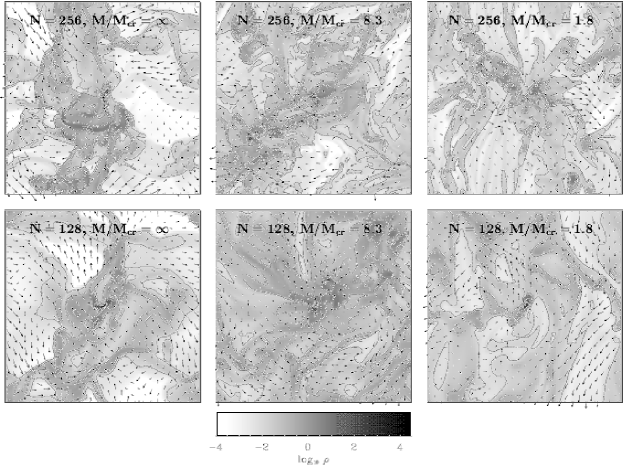
Figure 7: Two-dimensional slices of $256^{3}$ models from hmk01 driven with wavenumber $k=2$ hard enough that the mass in the box represents only 1/15 $\langle M_{\rm J}\rangle_{\rm turb}$, and with magnetic fields strong enough to give critical mass fractions as shown, corresponding to $\beta=\infty$, 0.9, and 0.04. Slices are taken at the location of the zone with the highest density at the time when $10$% of the total mass has been accreted onto cores. The plot is centered on this zone. Arrows denote velocities in the plane. The length of the largest arrows corresponds to a velocity of $v\sim 20c_{s}$. The density greyscale is given in the colorbar. (From hmk01 )

On the other hand, collapsing regions cannot be followed to scales less than one or two cells. We must again consider the resolution required for gravitational collapse. For a grid-based simulation, the criterion given by Truelove et al. t97 holds. Equivalent to the SPH resolution criterion, the mass contained in one grid zone has to be rather smaller than the local Jeans mass throughout the computation.

Applying this criterion strictly would limit our simulations to the very first stages of collapse, as we have not implemented anything like sink particles in ZEUS. We have therefore extended our models beyond the point of full resolution of the collapse, as we are primarily interested in the formation of collapsed regions, but not their subsequent evolution. Thus, in the ZEUS models, the fixed spatial resolution of the grid implies that strongly collapsed cores have a larger cross-section than appropriate for their mass. In encounters with shock fronts the probability for these cores to get destroyed or lose material is overestimated. Cores simulated with ZEUS are therefore more easily disrupted than they would be physically. SPH, on the other hand, underestimates the disruption probability, because sink particles cannot lose mass or dissolve again once they have formed. The physical result is thus bracketed by these two numerical methods.

We use the same driving method as described above for both the SPH and ZEUS models. We define an effective turbulent Jeans mass $\langle M_{\rm J}\rangle_{\rm turb}$ by substituting $c_{\rm s}^{2}\longrightarrow c_{\rm s}^{2}+1/3\,\langle v^{2}\rangle$ for the thermal sound speed $c_{\rm s}$ in equation (10) where we approximate the rms velocity of the flow $\langle v^{2}\rangle$ by $2E_{\rm kin}/M$. The turbulent Jeans mass $\langle M_{\rm J}\rangle_{\rm turb}$ must be compared to the total system mass $M\equiv 1$ in order to determine whether global stability is reached.

We find that local collapse occurs even when the turbulent velocity field carries enough energy to counterbalance gravitational contraction on global scales, as shown in Fig. 8. This confirms the results of two-dimensional (2D) and low-resolution ($64^{3}$) 3D computations with and without magnetic fields by Vázquez-Semadeni et al. vpp96 . An example of local collapse in a globally supported cloud is given in Figure 6. The presence of shocks in supersonic turbulence drastically alters the result from analytic models of incompressible turbulence, as was first noted by Elmegreen bge93 and studied numerically by Vázquez-Semadeni et al. vpp96 . The density contrast in isothermal shocks scales quadratically with the Mach number, so the shocks driven by supersonic turbulence create density enhancements with $\delta\rho\propto{\cal M}^{2}$, where ${\cal M}$ is the rms Mach number of the flow. In such fluctuations the local Jeans mass is decreased by a factor of $\cal M$ and therefore the likelihood for gravitational collapse increased.

Figure 8: Fraction of mass $M_{*}$ in dense cores as function of time. All models are computed using SPH with sink particles replacing dense, collapsed cores. The different model parameters from khm00 are indicated in the figure. The mass in the box is initially unity, so the solid curves are unsupported formally, while the others are supported. The figure shows how the efficiency of local collapse depends on the scale and strength of turbulent driving. Time is measured in units of the global system free-fall time scale $\tau_{\rm ff}$, while the driving wavelength $\lambda_{d}=2\pi/k$ (From khm00 )

To test this explanation numerically, we designed a test case driven at short enough wave length and high enough power to support even fluctuations with $\delta\rho\propto{\cal M}^{2}$, and ran it with both codes, driven with a wave number $k=39-40$. Within 20 $\tau_{\rm ff}$ this model shows no signs of collapse. All the other globally supported models with less extreme parameters that we computed did form dense cores during the course of their evolution, supporting our hypothesis that local collapse is caused by the density fluctuations resulting from supersonic turbulence.

Magnetic fields might alter the dynamical state of a molecular cloud sufficiently to prevent gravitationally unstable regions from collapsing mck99 . They have been hypothesized to support molecular clouds either magnetostatically or dynamically through MHD waves. Mouschovias & Spitzer ms76 derived an expression for the critical mass-to-flux ratio in the center of a cloud for magnetostatic support. Assuming ideal MHD, a self-gravitating cloud of mass $M$ permeated by a uniform flux $\Phi$ is stable if the mass-to-flux ratio

$$\frac{M}{\Phi}<\left(\frac{M}{\Phi}\right)_{cr}\equiv\frac{c_{\Phi}}{\sqrt{G}}.$$ (11)

with $c_{\Phi}$ depending on the geometry and the field and density distribution of the cloud. A cloud is termed subcritical if it is magnetostatically stable and supercritical if it is not. Mouschovias & Spitzer ms76 determined that $c_{\Phi}=0.13$ for a spherical cloud.

We include magnetic fields in our models of driven, self-gravitating turbulence to test their effectiveness in supporting against self-gravity. The MHD simulations start with a uniform magnetic field in the $z$-direction. We must consider the resolution required to accurately follow magnetized collapse. Numerical diffusion can reduce the support provided by a static or dynamic magnetic field against gravitational collapse. Increasing the numerical resolution decreases the scale at which numerical diffusion acts. For strong, subcritical fields, the resolution should ensure that numerical diffusion remains unimportant even for the dense, shocked regions. We did a suite of models varying the sound speed and the mass in the cube while holding the magnetic field strength constant, thus varying $M/M_{cr}$ and the number of zones in a Jeans length $\lambda_{J}$. From these models we conclude that for a self-gravitating magnetostatic sheet to be well resolved with the algorithm under study, its Jeans length must exceed four zones hmk01 .

Collapse occurs in both unmagnetized and magnetized cases at all resolutions, as shown in Figure 9.

Figure 9: Comparison of the mass accretion behaviour for runs driven at wavenumber $k=1-2$ with varying resolution. Pure hydro runs are shown in the upper panel, and MHD runs in the lower panel, with resolutions $64^{3}$ (dotted), $128^{3}$ (dashed), and $256^{3}$ (solid). $M_{*}$ denotes the sum of masses found in all cores determined by the modified clumpfind algorithm wgb94 ; khm00 . Note that these cores are subject to destruction as they can only collapse to the grid scale. Times are given in units of free-fall time. Although the collapse rate varies, we get collapse in all cases (From hmk01 )

However, increasing the resolution makes itself felt in different ways in hydrodynamical and MHD models. In the hydrodynamical case, higher resolution results in thinner shocks and thus higher peak densities. These higher density peaks form cores with deeper potential wells that accrete more mass and are more stable against disruption. If we increase the resolution in the MHD models, on the other hand, we can better follow short wavelength MHD waves, which appear to be able to delay collapse, although not to prevent it. This result extends to models with $512^{3}$ zones h01 .

5 Characterization of Turbulence

5.1 Wavelet Transforms

To obtain clues to the true physical nature of interstellar turbulence, characteristic scales and any inherent scaling laws have to be measured and modelled. A major problem with characterizing both the observations and the models is to determine what scaling behaviour, if any, is present in complex turbulent structures. Both the velocity and density fields need to be considered, but only the radial velocity and column densities can be observed.

One measure useful for characterizing structure and scaling in observed maps of molecular clouds is the $\Delta$-variance, $\sigma^{2}_{\Delta}$, an averaged wavelet transform method for measuring the amount of structure at different scales introduced by Stutzki et al. s98 . The $\Delta$-variance spectrum clearly shows characteristic scales and scaling relations, and its logarithmic slope can be analytically related to the spectral index of the corresponding Fourier power spectrum (see Fig. 10). In order to understand the physical significance of the characterization of the observational maps by $\Delta$-variance spectra, we apply the same analysis to observations of the Polaris Flare at three different scales f98 ; bp01 ; ht90 , as analyzed by s98 ; bso01 and to simulated observations of gas distributions resulting from our MHD models mo00 ; om02 , as well as to the actual density distributions from those models.

Figure 10: Comparison of 3D $\Delta$-variance spectra (above) to Fourier power spectra (below) for $128^{3}$ models of turbulence driven at wavenumbers of $k_{d}=2$ (solid), $k_{d}=4$ (dotted), and $k_{d}=8$ (dashed), demonstrating that the analytic relation between power spectrum slope and $\Delta$-variance spectrum slope also holds for the local behavior of structures not showing a straight power-law (From mo00 )

In Fig. 10 we compare the power spectrum and $\Delta$-variance for the density distibution from three simulations with different driving scales. Each shows a different characteristic scale formed by the driving, visible as a turn-over at large lags in the $\Delta$-variances and at small wavenumbers in the power spectrum, respectively. At smaller lags and higher wavenumbers power laws can be seen in both cases for the models with longer wavelength driving, with their slopes related by the analytic relation mentioned above. A steep drop-off follows at the smallest scales indicating the resolution limit of the simulation. The model with the shortest wavelength ($k_{d}=8$) driving shows no power law because the driving scale of 16 zones is only marginally larger than the dissipation scale of about 10 zones.

The $\Delta$-variance analysis of astronomical maps was extensively discussed by Bensch et al. bso01 . In all the observations they analyzed, the total cloud size was the only characteristic scale detected by means of the $\Delta$-variance. Below that size they found a self-similar scaling behaviour reflected by a power law with index $\alpha=$0.5–1.3 corresponding to a Fourier power spectral index $\zeta=$2.5–3.3.

In Fig. 11 we show how numerical resolution, or equivalently the dissipation scale, influences the $\Delta$-variance spectrum that we find from our simulations. We test the influence of the numerical resolution on the structure by comparing a simple hydrodynamic problem of decaying turbulence computed at resolutions from $64^{3}$ to $256^{3}$, with an initial rms Mach number $M=5$.

Figure 11: $\Delta$-variance of the density cubes (projected to two-dimensions) for a model of decaying hydrodynamic turbulence at a time $t/t_{s}=0.1$, where $t_{s}$ is the sound-crossing time, computed using numerical resolutions of $64^{3}$, $128^{3}$, and $256^{3}$ zones (From mo00 )

In contrast to the results from m99 which showed little dependence of the energy dissipation rate on the numerical resolution, we find here clear differences in the scaling behaviour of the turbulent structures. At small scales we find a very similar decay in the relative structure variations up to scales of about 10 times the pixel size (0.03, 0.06, and 0.1 for the resolutions $256^{3}$, $128^{3}$, and $64^{3}$, respectively) in all three models. This constant length range starting from the pixel scale clearly identifies this decay as being due to the numerical viscosity acting at the smallest available size scales.

Similar behaviour can be observed at the largest lags where structure variations decay for all three simulations at a length scale of roughly a quarter the cube size. This structure reflects the original driving of the turbulence with wavenumbers $1<k_{d}<8$, which produces structure on the corresponding length scales. Structures larger than about half the cube size are suppressed by the periodicity of the simulation cubes.

We can now attempt to interpret the observations using the behavior seen in the model $\Delta$-variance spectra, and equivalent behavior seen in velocity centroid $\Delta$-variance spectra of the models, as described by Ossenkopf & Mac Low om02 . Fig. 12 shows the square root of the $\Delta$-variance for the Polaris Flare velocity centroid maps. An upturn in power at the

Figure 12: The square root of the $\Delta$-variance of the smoothed Polaris Flare velocity centroid maps. The size of the smoothing filter was adapted to remove only the average noise level. Spectra are shown from three nested maps obtained with the 1.2 m CfA telescope with half power beam width (HPBW) 8.7’, the 3 m KOSMA with HPBW 2.2’, and the 30 m IRAM with HPBW 0.35’. At a distance of 150 pc, $1000^{\prime\prime}=0.73$ pc. (From om02 )

smallest lags in each map produced by the observational noise adding power at small scales was subtracted to prepare these spectra bso01 . The velocity structure in the Polaris Flare maps shows power-law behaviour from scales of about 0.05 to several parsecs. Below that range the slope of the $\Delta$-variance spectrum of the velocity centroids steepens, perhaps because of physical dissipation through ambipolar diffusion or other mechanisms, while above that range it flattens because of the lack of emission on larger scales. Bensch et al. bso01 demonstrated similar scaling behaviour in the intensity maps, reflecting the density structure.

Comparison between the observations of the Polaris Flare and the turbulence simulations constrains the mechanisms driving the turbulence in this cloud. Any mechanism that drives at an intermediate length scale, such as jets from embedded protostars, should produce a peak in the $\Delta$-variance at that scale, which is not observed. The approximately self-similar, power-law behaviour seen in the observations is best reproduced by models where the energy is injected at large scales and dissipated at small scales. Driving by interactions with superbubbles and field supernova remnants nf96 ; m02 would provide such a driving mechanism. The Polaris Flare molecular cloud lies in the wall of a large cylindrical structure representing one of the nearest H i supershells, the North Celestial Polar Loop m91 , adding additional support to this proposal.

The dominant physical mechanism for dissipation in molecular clouds was first shown by Zweibel & Josafatsson zj83 to be ambipolar diffusion. Klessen et al. khm00 showed that the length scale on which ambipolar diffusion will become important can be found by examining the ambipolar diffusion Reynolds number

$$R_{A}={\cal M}_{A}\tilde{L}\nu_{ni}/v_{A}$$ (12)

defined by Balsara b96 and Zweibel & Brandenburg zb97 , where $\tilde{L}$ and ${\cal M}_{A}$ are the characteristic length and Alfvén Mach number, $\nu_{ni}=\gamma\rho_{i}$ is the rate at which each neutral is hit by ions, and $v_{A}^{2}=B^{2}/4\pi\rho$ approximates the effective Alfvén speed in a mostly neutral region with total mass density $\rho=\rho_{i}+\rho_{n}$ and magnetic field strength $B$. The coupling constant depends on the cross-section for ion-neutral interaction, and for typical molecular cloud conditions has a value of $\gamma\approx 9.2\times 10^{13}$ cm³ s^-1 g^-1 (e.g. sm97 ).

Setting the ambipolar diffusion Reynolds number $R_{A}=1$ yields a diffusion length scale of

$$L_{D} = v_{A}/{\cal M}_{A}\nu_{ni}$$ (13)

$$\approx (0.041\mbox{pc}){\cal M}_{A}\left(\frac{B}{10\mbox{ $\mu$G}}\right)\!\left(\frac{10^{-6}}{x}\right)\!\left(\frac{10^{3}\mbox{ cm}^{-3}}{n_{n}}\right)^{3/2}$$ (14)

with the ionization fraction $x=\rho_{i}/\rho_{n}$ and the neutral number density $n_{n}=\rho_{n}/\mu$, with $\mu=2.36m_{H}$. If the ionization level in the Polaris Flare is low enough and the field is high enough, this length scale of order 0.05 pc would be directly resolved in the IRAM observations. We cannot yet unambiguously say whether the steepening observed at the smallest scales in the velocity spectra is due to beam smearing at the observational resolution limit or to a detection of the actual dissipation scale, similar to the downturn at the dissipation scale in the numerical models. If better observations do continue to show such a downturn in the future, that will be an indication of the dissipation scale.

5.2 Clump Characterization

Using 2D numerical simulations, Ballesteros-Paredes et al. bvs99 showed that observed clumps frequently come from the superposition of several physically disconnected regions in the line of sight at the same radial velocity (see also osg01 ) but not necessarily at the same position or three-dimensional velocity. This had earlier been suggested by workers including Burton b71 , Issa et al. imw90 , Falgarone, Puget, & Pérault f92 , and Adler & Roberts ar92 .

We used the models described above to examine this effect in 3D using simulated observations. We calculate the radiative transfer through the density and velocity fields given by the computations, assuming local thermodynamic equilibrium (LTE) for the population of the molecular energy levels, which is a sufficiently good approximation to study qualitatively the effects of projection and superposition (velocity crowding) of structure in the cloud. In order to determine differences when observing the same region with different tracers, we also set minimum density thresholds below which the molecules might be underexcited.

Velocity crowding contributes to the generation of clumps in the observational space, so observed clumps frequently contain emission from physically separated regions bvs99 ; p00 ; osg01 ; l01 . We demonstrate this effect using a typical MHD simulation with intermediate values of driving strength ($L=1$) and wavenumber ($k=4$).

Figure 13 shows physical and observed maps for ¹³CO(1-0) and (2-1). We see that clumps in real space (letters A, B, and C in panel $y-x(1-0)$) do not necessarily have a counterpart in observational space. Clumps in observational space, on the other hand, (letter D in panel $Vy-x(1-0)$) do not necessarily come from isolated regions in real space, but have contributions from many different regions along the same line of sight. In Figure 13 we plot dotted lines that show the places where the emission of a physical clump lies in observational space, and where the emission from an observational clump is generated in physical space. For reference, we use the same lines in the ¹³CO(1-0) map as in the ¹³CO(2-1) map.

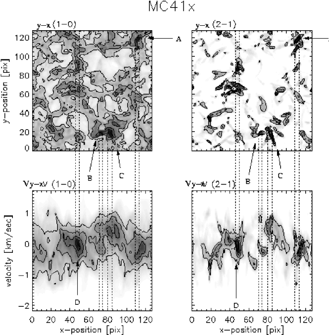
Figure 13: Physical and velocity space maps for ¹³CO(1-0) and (2-1) in a run with $\dot{E}=1$, $k=4$ and $B=0.1$. Clumps in physical space (A, B, C) do not necessarily correspond to clumps in the observed velocity space. Observed clumps in velocity space (D) are not necessarily formed by emission from a single region in physical space. From bm02

If clumps in the observational space are the result of the contribution of multiple regions in the physical space it is of primary importance to understand whether relationships reported for observed clumps in molecular clouds are also valid for the actual physical clumps.

Larson l81 studied the dependence with size of the mean density, velocity dispersion, and mass spectrum of the clouds in a sample of observational data taken from the literature. He found

$$\rho \propto R^{\alpha},$$ (15)

$$\delta v \propto R^{m},$$ (16)

$${dN\over d\log{M}} \propto M^{\gamma}.$$ (17)

The most commonly quoted values in the literature are $\alpha\sim-1$, $m\sim 1/2$, and $\gamma\sim-0.5$. However, there is some discrepancy in the values reported c87 ; l89 .

Larson l81 himself mentioned that the relationships he found might be due to the limitations of the observations. Kegel k89 first demonstrated that the observed mean density-size relationship could be due to observational effects, and that the observed and physical values of properties such as radius or volumetric density might be quite different. Scalo s90 showed that CO and extinction saturate at roughly the same column density, which forms the upper envelope of the mean density-size relationship. Vázquez-Semadeni et al. vbr97 reported the lack of a mean density-size relationship, confirming numerically the analysis by Kegel (k89 , see also the discussions in l81 and s90 ) in the sense that there are clouds with small sizes and low column density that will be undetected in observational surveys.

In Figure 14 we use the computational model described above to compare the density-size relationships in physical and observational spaces. We define clumps as a connected set of points below a local maximum following the intensity only downwards until the threshold is reached, a scheme implemented in the code called clumpfind wgb94 .

Figure 14: Mean density-size relationship for physical clumps in physical (PPP, upper panel); and simulated observational clumps in two different density tracers in observational coordinates (PPV, middle and lower panels). The dotted line has a slope of $\alpha=-1$. In physical space we find no correlation, verifying the results of Vázquez-Semadeni et al. vbr97 , but nevertheless the simulated observations show such a correlation, as found by Larson l81 and many others. The selection of two different density tracers was chosen to show that the apparent correlation does not depend on the selection of the density threshold. (From bm02 )

We note three points about Figure 14. First, there is no relation between mean density and size (eq. [15]), confirming the 2D results of Vázquez-Semadeni et al. vbr97 . Second, there is a minimum density below which there are no clumps identified. This minimum is just given by the density threshold we used in clumpfind. Third, even though the simulations exhibit a large dynamical range in density ($\rho_{\rm max}/\rho_{\rm min}\sim 3.5\times 10^{4}$), the dynamical range in the mean density-size relationship is small, because in constructing such a plot we choose the clumps around the local density maxima.

In the middle and lower panels of Fig. 14 we show the mean density-size relationship for clumps in simulated observational maps of the same run, integrated along the $x$ axis. The middle panel is the one obtained by using CS(1-0), and the lower panel is the relationship obtained by using ¹³CO(1-0). The observed clumps do exhibit approximately the relationship given by Larson l81 , despite the lack of correlation exhibited by the physical clumps in this model. We conclude from this demonstration that the observed density-size relationship (eq. [15]) is an observational artifact.

Kegel k89 suggested one mechanism that appears able to explain our results: only clouds with emission exceeding some intensity threshold will be detected, effectively setting a column density cutoff, rather than the physical density cutoff imposed in the physical density-size relationship. (This threshold is determined by the noise level in observations, or by some average intensity in the simulated observations). A constant column density cutoff produces a cutoff with slope $-1$ in the mean density-size plane (middle and lower panels), just as the constant physical density cutoff in physical space produces a flat cutoff.

6 Supernova-Driven Turbulence

Both support against gravity and maintenance of observed motions appear to depend on continued driving of the turbulence, as I have described. What then is the energy source for this driving?

Motions coming from gravitational collapse have often been suggested, but fail due to the quick decay of the turbulence as described above. If the turbulence decays in less than a free-fall time, then it cannot delay collapse for substantially longer than a free-fall time kb00 .

Protostellar jets and outflows are another popular suspect for the energy source of the observed turbulence. They are indeed quite energetic, but they deposit most of their energy into low density gas, as is shown by the observation of multi-parsec long jets extending completely out of molecular clouds bd94 . Furthermore, as described in the previous section, the observed motions show increasing power on scales all the way up to and perhaps beyond the largest scale of molecular cloud complexes om02 . It is hard to see how such large scales could be driven by protostars embedded in the clouds.

Another energy source that has long been considered is shear from galactic rotation. Work by Sellwood & Balbus sb99 has shown that magnetorotational instabilities bh91 ; bh98 could couple the large-scale motions to small scales efficiently. For parameters appropriate to the far outer H i disk of the Milky Way, they derive a resulting velocity dispersion of 6 km s^-1, close to that observed. This instability may provide a base value for the velocity dispersion below which no galaxy will fall. If that is sufficient to prevent collapse, little or no star formation will occur, producing something like a low surface brightness galaxy with large amounts of H i and few stars.

In active star-forming galaxies, however, clustered and field supernova explosions appear likely to dominate the driving, raising the velocity dispersion to the 10–15 km s^-1 observed in star-forming portions of galaxies (see work cited in m00 for example). These explosions will be predominantly from B stars no longer associated with their parent gas, as they are far more numerous than more massive O stars, have explosions that are just as powerful, and live long enough (up to 50 Myr) to either drift away from or ionize their parent clouds. This provides a large-scale self-regulation mechanism for star formation in disks with sufficient gas density to collapse despite the velocity dispersion produced by the magnetorotational instability. As star formation increases in such galaxies, the number of OB stars increases, ultimately increasing the supernova rate and thus the velocity dispersion, which will restrain further star formation.

Supernova driving not only determines the velocity dispersion, but may actually form molecular clouds by sweeping gas up in a turbulent flow. Clouds that are turbulently supported will experience inefficient, low-rate star formation, while clouds that are too massive to be supported will collapse ko01 , undergoing efficient star formation to form OB associations or even starburst knots.

We study supernova driving in a magnetized medium numerically, using the RIEMANN framework for computational astrophysics, which is based on higher-order Godunov schemes for MHD rb96 ; b98a ; b98b , and incorporates schemes for pressure positivity bs99a , and divergence-free magnetic fields bs99b . (The framework also includes parallelized, divergence-conserving, MHD adaptive mesh refinement bn01 ; b01 , though no results using that capability are shown here.) In the models presented here, we solve the ideal MHD equations including both radiative cooling and pervasive heating in a (200 pc)³ periodic computational box, using a grid of 128³ cells. We start the simulations with a uniform density of $2.3\times 10^{-24}$ g cm^-3, threaded by a uniform magnetic field in the $x$-direction with strength 5.8 $\mu$G, a factor of roughly two stronger than that observed in the Milky Way disk. This very strong field maximizes the effects of magnetization on the turbulence.

For the cooling, we use a tabulated version of the radiative cooling curve shown in Figure 1 of MacDonald and Bailey mb81 , which is based on the work of Raymond, Cox & Smith rcs76 and Shapiro and Moore sm76 . (It falls smoothly from temperatures of order $10^{5}$ K to $10^{2}$ K, not incorporating a sharp cutoff at $10^{4}$ K due to the turnoff of Ly$\alpha$ cooling.) In order to prevent the gas from cooling below zero, we set the lower temperature cutoff for the cooling at 100 K. We also include a diffuse heating term to represent processes such as photoelectric heating by starlight, which we set constant in both space and time. We set the heating level such that the initial equilibrium temperature determined by heating and cooling balance is 3000 K.

We explode SNe at a rate of one every 0.1 Myr in our box, twelve times higher than our present Galactic rate, corresponding to a mild starburst like M82. The SNe are permitted to explode at random positions. Each SN explosion dumps 10⁵¹ erg thermal energy into a sphere with radius 5 pc. The evolution of the system is determined by the energy input from SN explosions and diffuse heating and the energy lost by radiative cooling. An example of the resulting turbulence is shown in Figure 15.

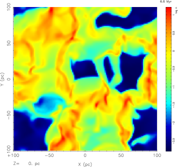
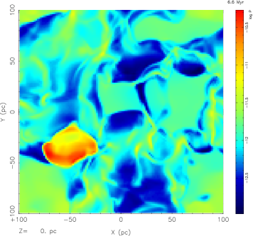
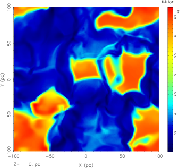
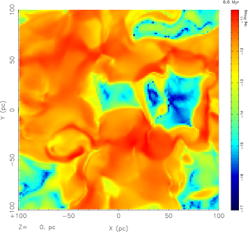
Figure 15: Two-dimensional slices through the three-dimensional MHD model M2, parallel to the magnetic field at a time of 6.6 Myr, showing density (upper left), thermal pressure (upper right), temperature (lower left), and magnetic pressure (lower right). Color bars indicate the scale of each quantity. (From m02 )

The first theories of the multi-phase ISM, such as Field, Goldsmith, & Habing fgh69 , postulated an isobaric medium. Since then, multi-phase models have commonly been interpreted as being isobaric, although McKee & Ostriker mo77 and Wolfire et al. w95 actually assume only local pressure equilibrium, not global, and McKee & Ostriker mo77 considered the distribution of pressures. In typical multi-phase models, the heating and cooling rates of the gas have different dependences on the temperature and density, so that the balance between heating and cooling determines allowed temperatures and densities for any particular pressure. This balance can be shown graphically in a phase diagram, showing, for example, the allowed densities for any pressure (fgh69 ; for a modern example, see Fig. 3(a) of w95 ).

In Figure 16, the thermal-equilibrium curve for the

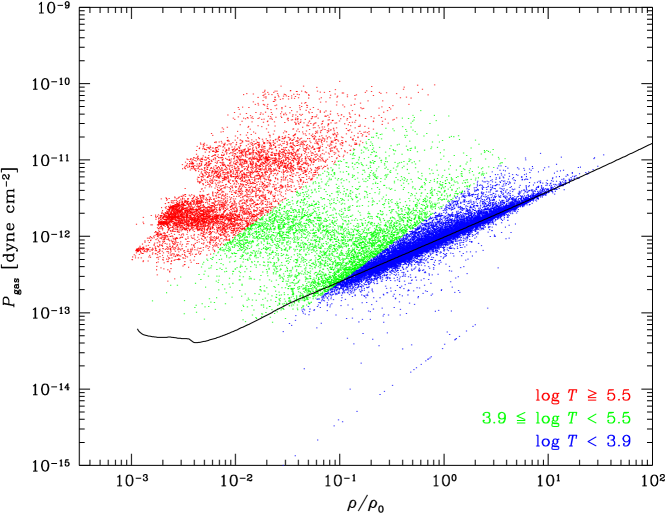
Figure 16: Scatter plot of pressure vs. density at $t=6.6$ Myrs in the MHD simulation M2, showing $32^{3}$ points sampled at intervals of four points in each direction. Note that for each density a wide variation in pressure is seen. Cool gas with $\log T<3.9$ is shown in blue, warm gas with $3.9<\log T<5.5$ in green, and hot gas with $\log T>5.5$ in red. The thermal equilibrium curve for the cooling and heating functions in this simulation is overlaid as a black line. (The line of points at the very bottom right corresponds to an absolute cutoff in the cooling at 100 K that was enforced on the temperature in this model.) Note that our cooling curve may artificially prevent much low-temperature gas from forming in this model. From m02

heating and cooling mechanisms included is shown as a black line. Only a single phase is predicted at high densities as our cooling curve did not include the physically-expected unstable region at temperatures of order $10^{3}$ K w95 . Thus, if our model produced an isobaric medium, it would be expected to have a single low-temperature phase in uniform density given by the point at which the thermal-equilibrium curve crosses that pressure level. (Effectively, we would have the hotter two of the three phases proposed by McKee & Ostriker mo77 .)

The scattered points in Figure 16 show the actual density and pressure of individual zones in the model. Many zones at low temperature do lie on the thermal equilibrium curve, but scattered all up and down it at many different pressures and densities. Furthermore, a substantial fraction of the gas has not had time to reach thermal equilibrium at all after dynamical compression. It appears that pressures are determined dynamically, and the gas then tries to adjust its density and temperature to reach thermal equilibrium at that pressure. Most gas will land on the thermal equilibrium curve when dynamical times are long compared to heating and cooling times.

Even if we include the proper physics to allow multiple phases, the behavior observed in our model will lead to all points within the range of pressures available along the thermal equilibrium line being occupied, rather than the appearance of discrete phases (also see the chapter by Vázquez-Semadeni et al. in this volume). Unstable regions along the thermal equilibrium curve g01 and off it will also be populated, as observed by Heiles cjh01 , but not as densely, as gas will indeed attempt to heat or cool to a stable thermal equilibrium at its current pressure. In particular, cold high pressure regions can be formed dynamically, without the influence of self-gravity, perhaps giving a method for forming molecular clouds with observed properties that are not in hydrostatic equilibrium.

The relation between magnetic and thermal pressure is shown in Figure 17. In this Figure, the relative strength of thermal and magnetic pressure is shown at one time for the magnetized simulation. The scattering of regions at very low thermal pressure all have substantial magnetic pressures, demonstrating that magnetically supported regions can occur. However, their relative importance is rather low, as shown by the small number of points in that regime. Hot gas can be seen, on the other hand, to be dominated by thermal pressure, with low magnetic pressures.

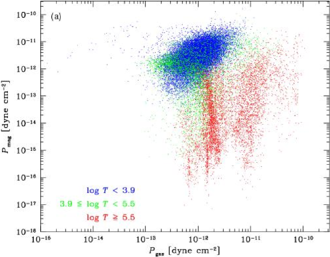
Figure 17: Scatter plot of magnetic vs. thermal pressure at $t=6.6$ Myrs in the MHD simulation. We again plotted a subset of $32^{3}$ points sampled at intervals of four points in each direction. Note that regions of very low thermal pressure have substantial magnetic pressures. From m02

As we have shown, the supernova-driven models have broad ranges of pressures. We can quantify this by examining the pressure probability density function (PDF), as shown in Figure 18. In both cases, these show roughly log-normal pressure PDFs, very unlike the power-law distributions predicted by the analytic theory derived by McKee & Ostriker mo77 .

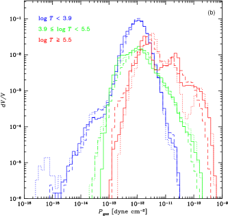
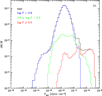
Figure 18: (b) Volume-weighted PDFs of pressure from the MHD models for cool gas with $\log T<3.9$ (blue), warm gas with $3.9<\log T<5.5$ (green), and hot gas with $\log T>5.5$ (red) at different times of 5.55 Myr (dashed), 6.06 Myr (dotted), and 6.55 Myr (solid) in the 1.6 pc resolution model M2. This model has twelve times the galactic rate of SNe, which results in a very broad pressure distribution. (c) Mass distribution of pressure for the MHD model M2 for the full distribution (black), and for cool gas with $\log T<3.9$ (blue), warm gas with $3.9<\log T<5.5$ (green), and hot gas with $\log T>5.5$ (red) at a time of 6.55 Myrs. Most of the mass is found in cold gas, with a broad distribution around the peak pressure. From m02

The observed distributions rather more resemble the log-normal density distributions suggested by Passot & Vázquez-Semadeni pv98 . Mac Low et al. m02 show that the cool gas can actually be modeled quite successfully with this heuristic theory.

7 Conclusions

• Even relatively strong magnetic fields, with the field in equipartition with the kinetic energy, cannot prevent the decay of turbulent motions on dynamical timescales far shorter than the observed lifetimes of molecular clouds. The significant kinetic energy observed in molecular cloud gas must be supplied more or less continuously.

• Supersonic turbulence strong enough to globally support a molecular cloud against collapse will usually cause local collapse. The turbulence establishes a complex network of interacting shocks. The local density enhancements in fluctuations created by converging shock flows can be large enough to become gravitationally unstable and collapse. The probability for this to happen, the efficiency of the process, and the rate of continuing accretion onto collapsed cores are strongly dependent on the driving wave length and on the rms velocity of the turbulent flow, and thus on the driving mechanism.

• Interstellar clouds driven on large scales or without even global turbulent support very rapidly form stars in clusters. On the contrary, in gas that is supported by turbulence, local collapse occurs sporadically over a large time interval, forming isolated stars. The total star formation efficiency before the cloud dissolves due to stellar feedback or external shocks will probably be low. Thus, the strength and nature of the turbulence may be fully sufficient to explain the difference between the observed isolated and clustered modes of star formation.

• Magnetorotational instabilities may provide a base value for the velocity dispersion below which no galaxy will fall. If that is sufficient to prevent collapse, little or no star formation will occur, producing something like a low surface brightness galaxy with large amounts of H i and few stars. In star-forming galaxies, however, clustered and field supernova explosions, predominantly from B stars no longer associated with their parent gas, appear likely to dominate the driving, raising the velocity dispersion to some 10–15 km s^-1.

• In a supernova-driven interstellar medium, we find a broad range of pressures with a log-normal distribution, and a substantial fraction of associated densities far from the thermal equilibrium values. This limits the predictive usefulness of phase diagrams based on thermal equilibrium, although thermal equilibrium at the local pressure will still be the mildly favored state. Gas pressures appear to be determined dynamically, and each individual parcel of gas seeks local thermal equilibrium at the pressure imposed on it by the turbulent flow. Inferences that molecular clouds must be gravitationally bound because of their high observed confinement pressures are called into question by these results. Regions with densities approaching the overall densities of GMCs, and pressures an order of magnitude above the average interstellar pressure appear in our simulations even in the absence of self-gravity.

I thank the referee of this review, E. Vázquez-Semadeni, for a detailed and thoughtful report, my collaborators M. A. de Avillez, J. Ballesteros-Paredes, D. Balsara, A. Burkert, F. Heitsch, J. Kim, R. S. Klessen, V. Ossenkopf, and M. D. Smith for their participation in different parts of the work reviewed here, and the organizers of the conference for their partial support of my attendance. This work was also partially supported by the NSF under CAREER grant AST99-85392 and by the NASA Astrophysical Theory Program under grant NAG5-10103. This research has made use of NASA’s Astrophysics Data System Abstract Service.

References

- (1) D. S. Adler, W. W. Roberts: Astrophys. J. 384, 95 (1992)
- (2) J. Arons, C. E. Max: Astrophys. J. 196, L77 (1975)
- (3) L. Armi, P. Flament: J. Geophys. Res. C, 90, 11779 (1985)
- (4) S. A. Balbus, J. F. Hawley: Astrophys. J. 376, 214 (1991)
- (5) S. A. Balbus, J. F. Hawley: Rev. Mod. Phys. 70, 1 (1998)
- (6) J. Ballesteros-Paredes, L. Hartmann, E. Vázquez-Semadeni: Astrophys. J. 527, 285 (1999)
- (7) J. Ballesteros-Paredes, M.-M. Mac Low: Astrophys. J., submitted (2002, astro-ph/0108136)
- (8) J. Ballesteros-Paredes, E. Vázquez-Semadeni, J. Scalo: Astrophys. J. 515, 286 (1999)
- (9) J. Bally, D. Devine: Astrophys. J. 428, L65 (1994)
- (10) D. S. Balsara: Astrophys. J. 465, 775 (1996)
- (11) D. S. Balsara: Astrophys. J. Supp. 116, 119 (1998a)
- (12) D. S. Balsara: Astrophys. J. Supp. 116, 133 (1998b)
- (13) D. S. Balsara: J. Comput. Phys. 174, 614 (2001)
- (14) D. S. Balsara, C. Norton: Parallel Comput. 27, 37 (2001)
- (15) D. S. Balsara, D. S. Spicer: J. Comput. Phys. 148, 133 (1999a)
- (16) D. S. Balsara, D. S. Spicer: J. Comput. Phys. 149, 270 (1999b)
- (17) M. R. Bate, I. A. Bonnell, N. M. Price: 1995, Monthly Not. Roy. Astron. Soc., 277, 362 (1995)
- (18) M. R. Bate, A. Burkert: Monthly Not. Roy. Astron. Soc. 288, 1060 (1997)
- (19) F. Bensch, J.-F. Panis, J. Stutzki, A. Heithausen, E. Falgarone: Astron. Astrophys. 365, 275 (2001)
- (20) F. Bensch, J. Stutzki, V. Ossenkopf: Astron. Astrophys. 366, 636 (2001)
- (21) W. Benz: in The Numerical Modelling of Nonlinear Stellar Pulsations. ed. by J. R. Buchler, (Kluwer, Dordrecht, 1990), p. 269
- (22) D. Biskamp, W.-C. Müller: Phys. Plasmas 7, 4889 (2000)
- (23) L. Blitz, F. H. Shu: Astrophys. J. 238, 148 (1980)
- (24) S. Bonazzola, E. Falgarone, J. Heyvaerts, M. Perault, J. L. Puget: Astron. Astrophys. 172, 293 (1987)
- (25) W. B. Burton: Astron. Astrophys. 10, 76 (1971)
- (26) J. S. Carr: Astrophys. J. 323, 170 (1987)
- (27) D. Clarke: NCSA Technical Report (1994)
- (28) T. Ebisuzaki, J. Makino, T. Fukushige, M. Taiji, D. Sugimoto, T. Ito, S. K. Okumura: Publ. Astron. Soc. Japan, 45, 269 (1993)
- (29) B. G. Elmegreen: Astrophys. J. 419, L29 (1993)
- (30) E. Falgarone, J.-F. Panis, A. Heithausen, M. Perault, J. Stutzki, J.-L. Puget, F. Bensch: Astron. Astrophys. 331, 669 (1998)
- (31) E. Falgarone, J.-L. Puget, M. Pérault: Astron. Astrophys. 257, 715 (1992)
- (32) G. B. Field, D. W. Goldsmith, H. J. Habing: Astrophys. J. 155, L149 (1969)
- (33) C. F. Gammie, E. C. Ostriker: Astrophys. J. 466, 814 (1996)
- (34) A. Gazol, E. Vázquez-Semadeni, F. J. Sánchez-Salcedo, J. Scalo: Astrophys. J. 557, L121 (2001)
- (35) L. Hartmann, J. Ballesteros-Paredes, E. A. Bergin: Astrophys. J. 562, 852 (2001)
- (36) J. F. Hawley, J. M. Stone: Comp. Phys. Comm., 89, 1 (1995)
- (37) C. Heiles: Astrophys. J. 551, L105 (2001)
- (38) A. Heithausen, P. Thaddeus: Astrophys. J. (Letters) 353, L49 (1990)
- (39) F. Heitsch, M.-M. Mac Low, R. S. Klessen: Astrophys. J. 547, 280 (2001)
- (40) F. Heitsch, E. G. Zweibel, M.-M. Mac Low, P. Li, M. L. Norman: Astrophys. J. 561, 800 (2001)
- (41) R. W. Hockney, J. W. Eastwood: Computer Simulation Using Particles (Institute of Physics, Bristol, England, 1988)
- (42) M. Issa, I. MacLaren, A. W. Wolfendale: Astrophys. J. 352, 132 (1990)
- (43) J. H. Jeans: Phil. Trans. A. 199, 1 (1902)
- (44) W. H. Kegel: Astron. Astrophys. 225, 517 (1989)
- (45) W.-T. Kim, E. C. Ostriker: Astrophys. J. 559, 70 (2001)
- (46) R. S. Klessen, A. Burkert: Astrophys. J. Supp. 128, 287 (2000)
- (47) R. S. Klessen, F. Heitsch, M.-M. Mac Low: Astrophys. J. 535, 887 (2000)
- (48) R. Larson: Monthly Not. Roy. Astron. Soc. 194, 809 (1981)
- (49) A. Lazarian, D. Pogosyan, E. Vázquez-Semadeni, B. Pichardo: Astrophys. J. 555, 130 (2001)
- (50) J. Léorat, T. Passot, A. Pouquet: Monthly Not. Roy. Astron. Soc. 243, 293 (1990)
- (51) R. B. Loren: Astrophys. J. 338, 902 (1989)
- (52) M.-M. Mac Low: Astrophys. J. 524, 169 (1999)
- (53) M.-M. Mac Low: in Stars, Gas, & Dust in Galaxies, ed. by D. Alloin, K. Olsen, G. Galaz (ASP, San Francisco, 2000), p. 55
- (54) M.-M. Mac Low, D. Balsara, M. A. de Avillez, J. Kim: Astrophys. J., submitted (2002, astro-ph/0106509)
- (55) M.-M. Mac Low, R. S. Klessen, A. Burkert, M. D. Smith: Phys. Rev. Lett. 80, 2754 (1998)
- (56) M.-M. Mac Low, V. Ossenkopf: Astron. Astrophys. 353, 339 (2000)
- (57) J. MacDonald, M. E. Bailey: Monthly Not. Roy. Astron. Soc. 197, 995 (1981)
- (58) C. F. McKee, J. P. Ostriker: Astrophys. J. 218, 148 (1977)
- (59) C. F. McKee: in The Origin of Stars and Planetary Systems, ed. by C. J. Lada and N. D. Kylafis (Kluwer, Dordrecht, 1999) p.29
- (60) H. Meyerdierks, A. Heithausen, K. Reif: Astron. Astrophys. 245, 247 (1991)
- (61) J. J. Monaghan: Ann. Rev. Astron. Astrophys. 30, 543 (1992)
- (62) T. Ch. Mouschovias: Astrophys. J. 211, 147 (1977)
- (63) T. C. Mouschovias, L. Spitzer: Astrophys. J. 210, 326 (1976)
- (64) C. A. Norman, A. Ferrara: Astrophys. J. 467, 280 (1996)
- (65) V. Ossenkopf, M.-M. Mac Low: Astron. Astrophys., in press (2002, astro-ph/0012247)
- (66) E. C. Ostriker, C. F. Gammie, J. M. Stone: Astrophys. J. 513, 259 (1999)
- (67) E. Ostriker, J. Stone, C. Gammie: Astrophys. J. 546, 980 (2001)
- (68) P. Padoan, and Å. Nordlund: Astrophys. J. 526, 279 (1999)
- (69) T. Passot, A. Pouquet, P. R. Woodward: Astron. Astrophys.197, 392 (1988)
- (70) T. Passot, & E. Vázquez-Semadeni: Phys. Rev. E 58, 4501 (1998)
- (71) T. Passot, E. Vázquez-Semadeni, A. Pouquet: Astrophys. J. 455, 536 (1995)
- (72) B. Pichardo, E. Vázquez-Semadeni, A. Gazol, T. Passot, J. Ballesteros-Paredes: Astrophys. J. 532, 353 (2000)
- (73) D. H. Porter, A. Pouquet, P. R. Woodward: Phys. Rev. Lett. 68, 3156 (1992)
- (74) D. H. Porter, A. Pouquet, P. R. Woodward: Phys. Fluids 6, 2133 (1994)
- (75) J. C. Raymond, D. P. Cox, B. W. Smith: Astrophys. J. 204, 290 (1976)
- (76) P. L. Roe, D. S. Balsara: SIAM J. Appl. Math. 56, 57 (1996)
- (77) J. Scalo: in Physical Processes in Fragmentation and Star Formation. ed. by R. Capuzzo-Dolcetta, C. Chiosi, A. di Fazio (Kluwer, Dordrecht, 1990) p. 151
- (78) J. A. Sellwood, S. A. Balbus: Astrophys. J. 511, 660 (1999)
- (79) F. H. Shu: Astrophys. J. 214, 488 (1977)
- (80) P. R. Shapiro, R. T. Moore: Astrophys. J. 207, 460 (1976)
- (81) M. D. Smith, M.-M. Mac Low: Astron. Astrophys. 326, 801 (1997)
- (82) M. Steinmetz: Monthly Not. Roy. Astron. Soc. 278, 1005 (1996)
- (83) J. M. Stone, M. L. Norman: Astrophys. J. Supp. 80, 753 (1992a)
- (84) J. M. Stone, M. L. Norman: Astrophys. J. Supp. 80, 791 (1992b)
- (85) J. M. Stone, E. C. Ostriker, C. F. Gammie: Astrophys. J. 508, L99 (1998)
- (86) J. Stutzki, F. Bensch, A. Heithausen, V. Ossenkopf, M. Zielinsky: Astron. Astrophys. 336, 697 (1998)
- (87) J. K. Truelove, R. I. Klein, C. F. McKee, J. H. Holliman II, L. H. Howell, J. A. Greenough: Astrophys. J. 489, L179 (1997)
- (88) E. Vázquez-Semadeni, J. Ballesteros-Paredes, L. F. Rodriguez: Astrophys. J. 474, 292 (1997)
- (89) E. Vázquez-Semadeni, T. Passot, A. Pouquet: Astrophys. J. 441, 702 (1995)
- (90) E. Vázquez-Semadeni, T. Passot, A. Pouquet: Astrophys. J. 473, 881 (1996)
- (91) M. G. Wolfire, C. F. McKee, D. Hollenbach, A. G. G. M. Tielens, E. L. O. Bakes, Astrophys. J. 443, 152 (1995)
- (92) J. P. Williams, E. J. de Geus, L. Blitz: Astrophys. J. 428, 693 (1994)
- (93) E. G. Zweibel, A. Brandenburg: Astrophys. J. 478, 563 (1997, err: 485, 920)
- (94) E. G. Zweibel, K. Josafatsson: Astrophys. J. 270, 511 (1983)