Bow Shocks from Neutron Stars: Scaling Laws and
HST Observations of the Guitar Nebula

Abstract

The interaction of high-velocity neutron stars with the interstellar medium produces bow shock nebulae, where the relativistic neutron star wind is confined by ram pressure. We present multi-wavelength observations of the Guitar Nebula, including narrow-band H$\alpha$ imaging with HST/WFPC2, which resolves the head of the bow shock. The HST observations are used to fit for the inclination of the pulsar velocity vector to the line of sight, and to determine the combination of spindown energy loss, velocity, and ambient density that sets the scale of the bow shock. We find that the velocity vector is most likely in the plane of the sky. We use the Guitar Nebula and other observed neutron star bow shocks to test scaling laws for their size and H$\alpha$ emission, discuss their prevalence, and present criteria for their detectability in targeted searches. The set of H$\alpha$ bow shocks shows remarkable consistency, in spite of the expected variation in ambient densities and orientations. Together, they support the assumption that a pulsar’s spindown energy losses are carried away by a relativistic wind that is indistinguishable from being isotropic. Comparison of H$\alpha$ bow shocks with X-ray and nonthermal, radio-synchrotron bow shocks produced by neutron stars indicates that the overall shape and scaling is consistent with the same physics. It also appears that nonthermal radio emission and H$\alpha$ emission are mutually exclusive in the known objects and perhaps in all objects.

1 INTRODUCTION

Bow shocks are observed on a wide variety of astrophysical scales, ranging from planetary magnetospheres (Spreiter & Stahara, 1995) and OB-runaway stars (van Buren & McCray, 1988) to merging galaxy clusters (Markevitch et al., 2002). They have been invoked in models for beamed gamma-ray bursts (Wang & Loeb, 2001), protostellar outflows (Ostriker et al., 2001), ultra-compact H II regions (van Buren & Mac Low, 1992) and the interaction of the solar wind with the interstellar medium (Baranov, Krasnobaev & Kulikovskii, 1971). Some of the most spectacular bow shock nebulae are those associated with neutron stars. The spindown of neutron stars (NS) transfers rotational kinetic energy into the interstellar medium, and bow shock nebulae provide a way to probe these energetic environments, revealing the properties of both the NS relativistic winds and the ambient interstellar medium (ISM).

The Guitar Nebula is one such visually striking bow shock nebula, produced by the radio pulsar B2224+65. The nebula was discovered in H$\alpha$ observations using the 5-m Hale Telescope at Palomar Observatory (Cordes, Romani & Lundgren, 1993). Until recently, there were only two other NS with bow shocks observed in H$\alpha$: B1957+20 (Kulkarni & Hester, 1988) and B0437$-$4715 (Bell et al., 1995). However, H$\alpha$ bow shocks have recently been discovered around a radio quiet NS, RX J1856.5$-$3754 (van Kerkwijk & Kulkarni, 2001), as well as another ordinary radio pulsar, B0740$-$28 (Jones, Stappers & Gaensler, 2002). More such nebulae will no doubt be discovered as targeted searches become more sensitive and cover more objects. Additionally, there are some bow shock nebulae which are detected at radio/X-ray wavelengths, but not in H$\alpha$, associated with known radio pulsars as well as radio-quiet NS: for example, the “Duck” (Frail & Kulkarni, 1991) is associated with the pulsar B1757$-$24 and the supernova remnant (SNR) G5.4$-$1.2, while the cometary nebula in the SNR IC 443 is produced by a radio quiet NS (Olbert et al., 2001).

In this paper, we derive scaling relationships for bow shock parameters based on the underlying physical processes, and discuss the requirements for such nebulae to be detectable. A detailed analysis of the Guitar Nebula is presented based on multi-wavelength observations, including high resolution Hubble Space Telescope (HST) observations which resolve the fine structure of the bow shock. Through model fitting, constraints are obtained on the density of the ambient ISM and the inclination of the NS velocity vector to the line of sight (LOS). The published data on NS bow shocks are consolidated with the parameters for the Guitar Nebula in order to test the derived scaling relationships for H$\alpha$ bow shocks. We verify that the stand-off angle for plerionic bow shock nebulae detected at radio and X-ray wavelengths also scales in the same manner. In testing these scaling laws, it is apparent that the current state of available information is inadequate, especially for radio-detected nebulae, leading to constraints on the ISM that are not very strong. We identify the sources of uncertainty, and suggest future observations that will be able to refine current constraints as well as confirm or refute physical scenarios relating to the formation of H$\alpha$ and plerionic bow shock nebulae.

The paper is organized as follows: the expected scaling relationships for bow shock parameters are derived in §2, along with an analysis of the detectability criteria for bow shock nebulae. Multi-wavelength observations of the Guitar Nebula are described in §3. Since the bright head of the Guitar Nebula is not resolved by ground-based optical images, high resolution HST observations are required to obtain bow shock parameters; these observations, and the associated model fitting, are described in §4. In §5, the derived scaling laws are tested for known NS bow shocks, with consolidated parameters for both H$\alpha$ and radio/X-ray bow shocks. Finally, in §6, we summarize our results, discuss their implications and identify future lines of inquiry.

2 SCALING LAWS FOR BOW SHOCK NEBULAE

Bow shock nebulae are produced when NS move supersonically through the ambient ISM, creating a shocked layer where ram pressure balance is established between the relativistic NS wind and the medium. As such, bow shock characteristics such as the stand-off angle between the NS and the tip of the bow shock should scale with the spindown energy loss rate of the NS and the density of the medium. Pulsars with detected H$\alpha$ bow shocks (J0437$-$4715, B0740$-$28, B1957+20 and B2224+65) have a wide range of properties, with $\dot{E}$ ranging over two orders of magnitude, and velocities and distances spanning an order of magnitude, as detailed in §5. This leads to the question of how the bow shock scales with changes in the properties of the NS and the ambient medium.

2.1 Scaling of the Stand-Off Angle

Wilkin (1996) provides an exact analytic solution for a stellar wind bow shock in the thin-shell limit, a problem first solved numerically by Baranov, Krasnobaev & Kulikovskii (1971). In this analytic treatment, ram pressure balance between the stellar wind and the ambient medium determines the stand-off radius of the bow shock ($R_{0}$). For a star moving with velocity $v_{\ast}$ through a uniform medium of density $\rho_{a}$, with a stellar wind mass loss rate $\dot{m}_{w}$ and wind velocity $v_{w}$, the condition for ram-pressure balance is

$$\rho_{a}v^{2}_{\ast}=\frac{\dot{m}_{w}v_{w}}{4\pi R_{0}^{2}},$$ (1)

leading to an expression for the stand-off radius,

$$R_{0}=\left(\frac{\dot{m}_{w}v_{w}}{4\pi\rho_{a}v^{2}_{\ast}}\right)^{1/2}.$$ (2)

For a relativistic NS wind, the momentum outflow per unit area ${\dot{m}_{w}v_{w}}$ can be recast as $\dot{E}/c$ under the assumption that the spindown energy loss is carried away by the relativistic wind. Then the stand-off radius becomes

$$R_{0}=\left(\frac{\dot{E}}{4\pi c\rho_{a}v^{2}_{\ast}}\right)^{1/2}.$$ (3)

The substitution of a relativistic NS wind in place of an isotropic stellar wind may be problematic, since the NS wind is at best only quasi-isotropic. Some authors have cited the possibility of an alignment of the NS spin axis and proper motion (e.g. Spruit & Phinney, 1998), and two pulsars (the Crab and Vela) apparently conform to this picture (Lai, Chernoff & Cordes, 2001), although it might not be a general phenomenon (Deshpande, Ramachandran & Radhakrishnan, 1999). In case of alignment, the rotation-averaged relativistic wind, while not isotropic, would be axisymmetric about the velocity vector, a situation which adds only one extra scaling parameter to the bow shock description (Wilkin, 2000). If there is no such alignment, so that the rotation vector is skewed with respect to both the velocity and the magnetic field, the behavior of the relativistic wind depends on the relative orientations of these vectors and the opening angle of the wind: for a range of orientations, rotational averaging leads to a quasi-isotropic situation relative to the velocity vector. Specifically, even for B2224+65, a relatively slow-spinning pulsar with a small stand-off radius $R_{0}$, the light cylinder radius (at which point the rotation-averaged NS wind has spread out over a large solid angle) is $\sim$ a few $\times 10^{-6}R_{0}$. In the absence of additional information, we adopt an isotropic description for the relativistic wind.

The observed stand-off angle $\theta_{0}$ is simply the projected stand-off radius at the NS distance:

$$\theta_{0}=R_{0}\sin i/D,$$ (4)

where $i$ is the inclination angle to the LOS, so that $i=\pi/2$ corresponds to a velocity vector in the plane of the sky, and $i=0$ corresponds to motion towards the observer. The measurable transverse velocity of the NS, $v_{\perp}$, is related to the actual velocity $v_{\ast}$ by the same projection factor:

$$v_{\perp}=\mu D=v_{\ast}\sin i,$$ (5)

where $\mu$ is the measured angular proper motion. The ambient density of the ISM, $\rho_{a}$, is the product of the number density of the medium ($n_{\rm H}$), the mass of the H atom ($m_{\rm H}$) and the equivalent molecular weight of the hydrogen and helium mixture ($\gamma_{\rm H}$ = 1.37 for cosmic abundances, with 27% He by mass). Defining $n_{\rm A}$, the density in atomic mass units per unit volume,

$$\rho_{a}=n_{\rm H}\gamma_{\rm H}m_{\rm H}=n_{\rm A}m_{\rm H}.$$ (6)

Making the appropriate substitutions in Eqn. 3, and factoring in terms of constants, unknown quantities and observables, we obtain:

$$\theta_{0}=\left(4\pi m_{\rm H}c\right)^{-1/2}\left(\frac{\sin^{2}i}{n_{\rm A}^{1/2}}\right)\left(\frac{\dot{E}^{1/2}}{\mu D^{2}}\right);$$ (7)

the last factor comprises the quantities $\dot{E}$, $D$ and $\mu$, which are (at least in principle) directly measurable. Eqn. 7 can be evaluated numerically, for $\theta_{0}$ in milliarcsecond, $\dot{E}_{33}$ in $10^{33}$ erg s^-1, $D$ in kpc, $\mu_{100}$ in 100 milliarcsecond yr^-1 and $n_{\rm A}$ in cm^-3:

$$\theta_{0}=56.3\,{\rm mas}\left(\frac{\sin^{2}i}{n_{\rm A}^{1/2}}\right)\left(\frac{\dot{E}_{33}^{1/2}}{\mu_{100}D_{\rm kpc}^{2}}\right).$$ (8)

2.2 Scaling of the H$\alpha$ Flux

Bow shocks emit H$\alpha$ photons when the partially neutral ISM encounters the shock front, traveling at the NS velocity $v_{\ast}$. The neutral atoms are not immediately affected by the shock transition, but undergo collisional excitation and ionization in the hot post-shock flow due to encounters with shocked electrons and protons (Chevalier & Raymond, 1978). H$\alpha$ emission is proportional to the probability of an excitation before ionization, which is given by the ratio of the excitation rate $q_{\rm ex}$ to the ionization rate $q_{\rm i}$ (Raymond, 1991). The observed rate of H$\alpha$ emission ($F_{\alpha}$) from a nebula which subtends a solid angle $\Delta\Omega$ is given by:

$$F_{\alpha}=\frac{q_{\rm ex}}{q_{\rm i}}\;n_{\rm H\,\scriptscriptstyle{I}}v_{\ast}\;\frac{\Delta\Omega}{4\pi g_{{\rm H}\alpha}},$$ (9)

where $g_{{\rm H}\alpha}$ is the extinction correction for H$\alpha$ ($\approx 3$ for the Guitar Nebula), and Raymond (1991) gives $q_{\rm ex}/q_{\rm i}\approx 0.2$ H$\alpha$ photons per neutral atom.

The solid angle subtended by the bow shock nebula $\Delta\Omega\sim(\eta R_{0}/D)^{2}$, where $\eta$ is a geometric factor which depends on the NS velocity. Cordes, Romani & Lundgren (1993) use $\eta\propto v_{\ast}$, which is physically plausible, since a faster-moving NS sweeps up a larger volume of ISM within the shock front during the ionization timescale, so that $\Delta\Omega\propto v_{\ast}^{2}$. To retain generality, we use $\eta\propto v_{\ast}^{\beta}$, which implies $\Delta\Omega\propto v_{\ast}^{2\beta}(R_{0}/D)^{2}$. In addition, defining the neutral fraction $X=n_{\rm H\,\scriptscriptstyle{I}}/n_{\rm H}$ leads to $n_{\rm H\,\scriptscriptstyle{I}}=Xn_{\rm H}\propto X\rho_{a}$, and substituting for $\Delta\Omega$ and $n_{\rm H\,\scriptscriptstyle{I}}$ in Eqn. 9,

$$F_{\alpha}\propto Xn_{\rm H}\,v_{\ast}(\eta R_{0}/D)^{2}.$$ (10)

The H$\alpha$ photons are emitted isotropically by collisionally excited neutral atoms, so that geometric projection of the stand-off radius and the nebula itself does not affect the total observed flux $F_{\alpha}$, but projection effects have to be accounted for to express the actual NS velocity $v_{\ast}$ in terms of the observables $\mu$ and $D$. Thus the H$\alpha$ flux can be expressed in terms of observable quantities ($\theta_{0},\mu,D$) and unknowns ($\sin i,n_{\rm H},X$):

$$F_{\alpha}\propto Xn_{\rm H}\,\theta_{0}^{2}{v_{\ast}}^{2\beta+1}\;\propto Xn_{\rm H}\,\theta_{0}^{2}\left(\frac{\mu D}{\sin i}\right)^{2\beta+1}.$$ (11)

Alternatively, using the definition of $R_{0}$ from Eqn. 3, a scaling relationship can be derived for the observed H$\alpha$ flux in terms of measurable quantities and the unknown neutral fraction:

$$F_{\alpha}\propto\frac{X\dot{E}v_{\ast}^{2\beta-1}}{D^{2}},$$ (12)

which reduces to the expression derived by Cordes, Romani & Lundgren (1993) for $\beta=1$.

2.3 Detectability of H$\alpha$ Bow Shock Nebulae

For bow shock nebulae, the observed H$\alpha$ emission comes from the outer shocked layer, where the neutral medium is swept up and collisionally excited. There is also an inner shocked region which encloses the relativistic NS wind and may produce synchrotron radiation detectable in X-ray or radio observations. H$\alpha$ emission requires the existence of a significant neutral component in the medium, which is true for only $\sim 20\%$ of the ISM (McKee & Ostriker, 1977). Thus the non-detection of a nebula in H$\alpha$ may reflect pre-ionization of the ISM by supernovae, or thermal radiation from the NS or shocked gas, and places an upper limit on the neutral fraction present in the ambient medium. This is especially applicable for nebulae detected at radio/X-ray wavelengths, but not seen in H$\alpha$.

Detection criteria can be formulated in order to predict whether a pulsar should produce a bow shock nebula visible in H$\alpha$. Considering the average flux per detector pixel, the ratio of the H$\alpha$ flux to the angular size of the nebula, $F_{\alpha}/\Delta\Omega$, must exceed a (detector dependent) threshold:

$$\frac{F_{\alpha}}{N_{\rm pixel}}=\frac{F_{\alpha}}{\Delta\Omega/\Delta_{\rm CCD}}>S_{\rm thresh}.$$ (13)

From Eqn. 9, this implies that $Xn_{\rm H}v_{\ast}/g_{{\rm H}\alpha}$ must exceed a limiting value, a result independent of the spindown flux $\dot{E}/D^{2}$. However, a criterion based on the average flux does not account for brightness variations within the nebula, which can be substantial (as seen, for example, in the Guitar Nebula, discussed in §3). The optimal detection method is to block average all pixels which contain nebular emission, in which case (assuming uncorrelated random noise in each pixel) the average flux per detector pixel only needs to exceed $S_{\rm thresh}/\sqrt{N_{\rm pixel}}$ for a detection:

$$\frac{F_{\alpha}}{N_{\rm pixel}}>\frac{S_{\rm thresh}}{\sqrt{N_{\rm pixel}}}.$$ (14)

It is worth noting, however, that the optimal averaging size may not be known in advance, and a computationally intensive search may be required. For optimal detection, again using Eqn. 9 and substituting for the angular size of the nebula,

$$\frac{Xn_{\rm H}^{1/2}}{g_{{\rm H}\alpha}}\frac{\dot{E}^{1/2}v_{\ast}^{\beta}}{D}>\kappa\,S_{\rm thresh},$$ (15)

where $\kappa$ encapsulates various constants and numerical factors. As expected, H$\alpha$ bow shock nebulae are more likely to be detected for pulsars with larger spindown flux and higher velocities, located in regions with higher neutral fractions and lower extinction.

The detection criterion formulated in Eqn. 15 can be recast in terms of the minimum NS velocity required to produce a detectable bowshock, given the spindown flux and the ambient ISM. For concreteness, we assume a telescope sensitivity comparable to the 5-m Hale Telescope at Palomar, as used to detect the Guitar Nebula (§3), and $\beta=1$ as before. Then, for $D$ in kpc, $\dot{E}$ in units of 10³³ erg s^-1, and $n_{\rm H}$ in cm^-3,

$$V_{\rm min}=14\;{\rm km\;s}^{-1}\frac{g_{{\rm H}\alpha}}{Xn_{\rm H}^{1/2}}\left(\frac{\dot{E}_{33}}{D^{2}_{\rm kpc}}\right)^{-1/2}.$$ (16)

The relationship derived for the minimum required velocity is plotted in Fig. 1, along with transverse velocities for all pulsars with measured proper motions. All known bow shock nebulae are marked on the plot: their locations confirm the applicability of the detection criterion developed above. As mentioned above, the X-ray and radio-detected bow shock nebulae which are not detected in H$\alpha$ provide upper limits on the neutral fraction present in the ambient medium. The plot also identifies future candidates for deep searches for bow shock nebulae, although the uncertainties in the distance and velocity estimates for most pulsars and the large range of plausible values for $Xn_{\rm H}^{1/2}/g_{{\rm H}\alpha}$ are likely to limit its usefulness as a strong predicting tool.

Figure 1: Detectability of bow shock nebulae. Transverse velocities are plotted against the spindown flux $\dot{E}/D^{2}$ for all pulsars with published proper motions. The velocity and distance estimates are significantly better for pulsars with parallax distances, which are plotted with larger open circles. Lines are overplotted for the detection criterion in Eqn. 16, for $Xn_{\rm H}^{1/2}/g_{\alpha}=0.01$ (dashed) and 0.1 (dotted). All known H$\alpha$ and radio / X-ray bow shock nebulae are identified on the plot. The Crab (B0531+21) and Vela (B0833$-$45) pulsars are not detected as bow shock nebulae because of the negligible neutral fraction in their local ISM.

3 MULTI-WAVELENGTH OBSERVATIONS OF THE GUITAR NEBULA

The visually spectacular Guitar Nebula is a bow shock nebula produced by the otherwise unexceptional pulsar B2224+65 ($P=0.68$ s, $\dot{P}=9.7\times 10^{-15}$ s s^-1). The spindown luminosity of the pulsar ($\dot{E}=10^{33.08}$ erg s^-1, assuming a moment of inertia of $10^{45}$ gm cm²) is significantly lower than the $\dot{E}$ of other pulsars with known H$\alpha$ bow shocks. However, B2224+65 has an extremely large space velocity, which evidently compensates for the low $\dot{E}$ in producing a visible bow shock nebula. Its proper motion $\mu=182\pm 3$ mas yr^-1, at a position angle $52.1\arcdeg\pm 0.9\arcdeg$ (Harrison, Lyne & Anderson, 1993). The dispersion measure (DM = 36.16 $\pm$ 0.05 pc cm^-3) of the pulsar, combined with a model for the Galactic electron density distribution (Taylor & Cordes, 1993) yields a distance $D\approx 2.0\pm 0.5$ kpc, at which the transverse velocity $v_{\perp}=D\mu\approx(1.7\pm 0.4)\times 10^{3}$ km s^-1, the largest known velocity among radio pulsars.

It is evident from the discovery images that there may be a significant amount of ionized material in the vicinity of the pulsar, biasing the DM upward, and hence the distance may be overestimated. However, even at a distance of 1 kpc, the pulsar velocity ($\gtrsim 850$ km s^-1) is significantly higher than the mean population velocity of $\sim 450$ km s^-1 estimated by Lyne & Lorimer (1994). Recent studies (Arzoumanian, Chernoff & Cordes, 2001; Cordes & Chernoff, 1998) prefer a bimodal velocity distribution, with a significant portion ($\sim 15\%$) of pulsars having a space velocity $>1000$ km s^-1. B2224+65 is probably at the high end of this distribution, and the bow shock nebula is visible in spite of the small $\dot{E}$ due to the large space velocity of the pulsar.

3.1 Ground-based Optical Observations

In an ongoing program at Palomar Observatory, the Guitar Nebula has been imaged regularly at the 5-m Hale Telescope using the Carnegie Observatories Spectroscopic Multislit and Imaging Camera (COSMIC; Kells et al., 1998), mounted at the f/3.5 prime focus, in reimaging mode. A narrow-band H$\alpha$ filter (20 Å at 6564 Å) was used. The typical seeing was $\sim 0.9\arcsec$–$1.4\arcsec$, significantly larger than the CCD pixel scale (0.4″). The CCD data were processed in standard ways with IRAF tasks. Data obtained in 1995 were combined (9000 s total integration time) to produce the representative image presented in Fig. 2.

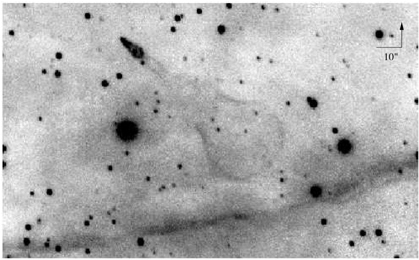
Figure 2: The Guitar Nebula in H$\alpha$ (20 Å filter at 6564 Å), imaged with the 5-m Hale Telescope at Palomar Observatory in mid-1995. North is up and east is to the left, as indicated, and the L has arms 10″ in size.

The Palomar image of the Guitar Nebula shows a remarkable structure consisting of a faint, limb-brightened “guitar body” which is approximately symmetric, with an elongated neck and a bright head, the tip of which coincides with the location of the pulsar. The axis of the nebula matches the position angle of the pulsar proper motion ($52.1\arcdeg\pm 0.9\arcdeg$), as expected. Differential Galactic rotation causes only a small effect ($<3\%$ of the transverse velocity) and is therefore neglected.

The body of the guitar appears to be composed of two closed-off bubbles. This could be explained by the projection of an open structure onto the plane of the sky, or by episodic variation in $\dot{E}$, which is not inconceivable given that B2224+65 has been known to glitch. The complex shape may alternatively be explained by the penetration of neutral ISM atoms into the space occupied by the pulsar wind, as suggested by Bucciantini & Bandiera (2001). However, the simplest explanation is the existence of density variations in the ambient medium. The observed closed bubble structures can be produced by density gradients oriented roughly parallel to the NS transverse velocity. The nebula brightens where it narrows between the two bubbles, as expected in a higher density region. The extremely bright head is then created by the NS entering a region with much higher ($\sim 10\times$) density, or a significantly higher neutral fraction. The distinct variations in brightness along the nebula, the observed departures from symmetry on small scales and the existence of large-scale filamentary structures (visible at the bottom of Fig. 2) can all be explained within this scenario, although other explanations cannot be ruled out.

3.2 Radio Interferometric Observations

The Guitar Nebula was observed at radio wavelengths with the NRAO Very Large Array (VLA). In order to get comparable resolutions over a range of frequencies, different VLA configurations were used: B-array for 1.4 GHz and 4.8 GHz, and C-array for 8.4 GHz observations. About 3 hours of integration time were obtained at each frequency, though the 8.4 GHz observation was plagued by poor weather conditions and did not yield as much usable data as the other frequencies. The observation parameters are summarized in Table 1.

The data were deconvolved using the CLEAN algorithm (Högbom, 1974), as implemented in AIPS, the Astronomical Image Processing System, in order to remove the sidelobes of strong sources within the primary beam. Wide-field images were produced at each frequency with map noise ranging from 23 $\mu$Jy to 28 $\mu$Jy, as detailed in the last column of Table 1.

Table 1: Multi-array Radio Observations at the VLA

$\nu_{\rm obs}$	VLA	Beam	Tint	$\Delta\nu$	$\sigma$ (RMS)
(GHz)	Array	(″)	(hr)	(MHz)	($\mu$Jy/beam)
1.4	B	3.8	2.9	50	27
4.9	B	1.2	2.9	50	23
8.4	C	2.2	2.4	100	28

The radio pulsar B2224+65 is detected at 1.4 GHz as a point-source with a flux $\sim$ 3.2 mJy. It is undetected at the higher frequencies. No extended features related to the Guitar Nebula or the optical filamentary structures are observed. We derive an upper limit ($\sim 5\sigma$) of 0.1 mJy beam^-1 on any synchrotron emission, either from the relativistic pulsar wind, or from the shock accelerated particles in the nebula, at wavelengths between 1.4 and 8.4 GHz with 1–4″ beam sizes. The non-detections thus rule out any plerionic component to the pulsar or any non-thermal emission from the Guitar Nebula over the observed range of wavelengths and resolutions. The data were also smoothed by tapering in the $U-V$ domain: although the possibility of faint extended emission on much larger scales cannot be excluded, no significant flux was detected from the Guitar Nebula after smoothing to 2–8″ beam sizes, comparable to the size of the bright part of the nebula in H$\alpha$.

The derived upper limit on plerionic radio emission is more stringent than those derived by Gaensler et al. (2000) for other pulsars, and the non-detection is consistent with their conclusion that older pulsars may become less efficient at producing synchrotron emission with increasing age.

3.3 X-ray and Infra-Red Observations

X-ray observations of the Guitar Nebula using the ROSAT High Resolution Imager have been described by Romani, Cordes & Yadigaroglu (1997). Weak soft X-ray emission is detected using an aperture mask matched to the optical nebula, but the detection is significant at only $\sim 4\sigma$. Follow-up observations using Chandra have recently been obtained, and will be described elsewhere.

Narrow-band infrared observations with PFIRCAM at the Hale 5-m telescope at Palomar Observatory resulted in non-detections, which complement the radio observations in limiting any thermal or non-thermal emission from the Guitar Nebula. Upper limits on the infrared flux will be published in future work.

4 HUBBLE SPACE TELESCOPE OBSERVATIONS AND MODELING

The head of the Guitar Nebula is not well resolved by ground-based observations, and the expected scale of the shocked region where the NS wind meets the ambient medium ($\sim 0.05\arcsec$) cannot be probed from the ground. HST observations are required, followed by model fitting to obtain the bow shock parameters.

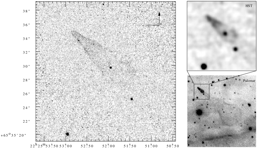
Figure 3: The head of the Guitar Nebula, imaged with the HST Planetary Camera (7200 seconds, 22 Å filter at 6564 Å) in late 1994. The left panel shows a section of the image with a hyperbolic-sine stretch applied to the grayscale. The lower right panel marks the region covered by the image section, superimposed on the near-contemporaneous Palomar image (mid 1995). The upper right panel shows the HST image convolved with the typical seeing disk ($\sim 1\arcsec$ FWHM) at Palomar, which makes the bright head and the neck of the Guitar visible. For reference, the three bright stars in the HST images are also visible on the Palomar image (Fig. 2). (Image degraded to fit astro-ph size limits)

4.1 HST Observations

High-resolution HST observations were obtained in 1994 December, using the Wide Field and Planetary Camera 2 (WFPC2; Holtzman et al., 1995). The bright head of the nebula was centered on the Planetary Camera (PC), which provides 0.0455″ resolution. The observations include 6 dithered exposures of 1200 seconds each, using filter F656N (22 Å at 6564 Å), comparable to the filter used at Palomar. The images were combined using Variable-Pixel Linear Reconstruction (or ‘Drizzling’), as described by Fruchter & Hook (2002). This includes cosmic ray rejection and partially compensates for the undersampling of the HST point-spread function by the 0.0996″ pixels of the WF chips on WFPC2.

A section of the PC image is presented in Fig. 3: for reference, the three stars visible in the frame are also seen in the Palomar image (Fig. 2). In spite of the limited signal-to-noise ratio (S/N) of the image, it is apparent that the bright head of the Guitar Nebula, unresolved in the Palomar images, is resolved by the PC. The bow shock is limb-brightened, as observed in the extended Guitar body observed at Palomar. The bright head and the neck of the Guitar become visible when the PC image is smoothed down to the typical seeing at Palomar, as shown in the upper right panel of Fig. 3. The extended body of the Guitar and the nearby filamentary structures are also detected in the WF images after smoothing (not shown here).

Along with the narrow-band images, broad-band images were also obtained with WFPC2, with 4 dithered exposures of 180 seconds each using filter F675W (867 Å at 6717 Å). The combined image (720 s) shows no significant emission from the nebula. As expected, no optical counterpart is detected for the radio pulsar, down to a limiting magnitude of $R=25.8$ ($5\sigma$) on the broad-band PC image.

4.2 Evolution of the Guitar Nebula

As discussed above, the simplest explanation for the characteristic shape of the Guitar Nebula is the propagation of the NS through a non-uniform ambient medium, in which case the shape of the nebula provides information about the density of the medium encountered in the past.

Fig. 4 shows the symmetric and anti-symmetric components of the head of the Guitar Nebula, which were obtained by mirroring a smoothed version of the PC image about the axis of the nebula and taking the sum and the difference of the two. The axis was found by using the pulsar proper motion as a starting point, and then fitting for the bow shock position angle, as described below. The symmetric component of the image shows significant changes in the opening angle of the nebula at 2″ scales, which are also visible, though less prominent, in the unsmoothed HST image (Fig. 3). It appears that the opening angle has narrowed recently ($\lesssim 10$ yr, between 1 and 2″ downstream from the tip), probably as the NS encountered a gradient of increasing density.

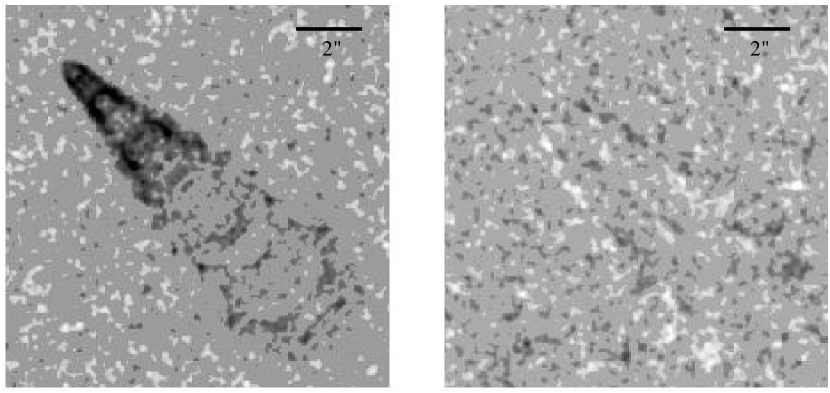
Figure 4: Symmetric and anti-symmetric components of the head of the Guitar Nebula, obtained by mirroring the head of the nebula about its axis. The image has been enhanced to bring out detail by assigning the mean amplitude to all pixels with amplitudes within $\pm 1\sigma$ of the image mean. The range of the greyscale is the same for both panels. While the tip of the head is almost perfectly symmetric, the limbs of the nebula are visible in the anti-symmetric image at the $\pm 2\sigma$ level.

There is also a small but significant departure from bilateral symmetry along the head of the Guitar Nebula, as illustrated by the image of the anti-symmetric component. The tip of the head is almost perfectly symmetric, and disappears in the anti-symmetric image, but the north-west and south-east limbs of the nebula deviate from the axis of symmetry at the $2\sigma$ level, consistent with a density gradient in the ambient medium which is not aligned with the NS velocity.

In both the smoothed HST image (Fig. 3) and the image of the symmetric component, the head of the nebula appears to have a closed-off structure, reminiscent of the rounded end of the “guitar body” seen on the Palomar image (Fig. 2). Once again, while various other explanations (including a time-variable $\dot{E}$) cannot be ruled out, the simplest explanation involves the existence of a density gradient, which confines the expansion of the head of the nebula. This explains both the brightening of the head of the nebula and the faint tubular “neck” of the guitar.

As part of an ongoing effort to monitor the evolution of the nebula, several images have been obtained at the 5-m Hale Telescope at Palomar Observatory over the past 7 years. Additionally, we expect to obtain another HST observation at higher S/N in late 2001, at which time the NS will have moved $\sim 1\arcsec$ from the previous position. This will allow a detailed study of the dynamic evolution of the head of the nebula and the ISM in the neighborhood of the NS, or alternatively, more exotic scenarios with time-variable $\dot{E}$.

4.3 Modeling the Bow Shock

The lack of an optical counterpart to PSR B2224+65 makes it difficult to obtain bow shock parameters like the stand-off angle $\theta_{0}$ by inspection of the image. Model fitting must be used in order to extract $\theta_{0}$ from the HST image, which resolves the stand-off region at the head of the bow shock.

Adopting the simple momentum-conserving description from Wilkin (1996), the shape of the bow shock can be expressed in polar coordinates ($R,\theta$) with the NS at the origin and traveling along the $\hat{z}$ axis:

$$R(\theta)=\frac{\sqrt{3}R_{0}}{\sin\theta}\left(1-\frac{\theta}{\tan\theta}\right)^{1/2}.$$ (17)

This expression describes the shape of a thin shell bow shock provided that the shocked gas undergoes rapid radiative cooling. If the cooling is not rapid enough, thermal pressure should result in a somewhat wider tail downstream along the bow shock. The momentum-conserving description also assumes mixing in the shocked layer between the ambient medium and the relativistic wind, whereas a laminar flow may be a more accurate description (Bucciantini & Bandiera, 2001). The model also assumes an ambient medium with uniform density, which, we have argued, is not the case here. However, the present work is limited to extracting basic bow shock parameters from an image with poor S/N. To work around these limitations, the model fitting procedure was restricted to within 2.6″ of the tip of the bright head, where the opening angle does not change much, the surface is relatively smooth, and the behavior of the tail downstream is not relevant.

The thin shell bow shock described by Eqn. 17 can be scaled and projected to account for viewing geometry. For each set of scale and geometry parameters, the projected surface density is calculated by integrating the density through the bow shock along each line of sight. The H$\alpha$ flux from the nebula is proportional to the projected surface density, accounting for the observed limb-brightened appearance.

A bow shock nebula described by this model can be parameterized by two angles, the inclination angle of $\hat{z}$ to the LOS ($i=0$ for motion towards the observer, and $i=\pi/2$ for motion in the plane of the sky), and a position angle on the sky, measured east of north. Additional parameters are the thickness of the shocked layer which emits in H$\alpha$ as a fraction of the stand-off radius, a constant numerical factor which relates the H$\alpha$ flux to the projected surface density, and a dimensionless scale parameter,

$$S=D^{-2}_{\rm kpc}\,n_{\rm A}^{-1/2}(\dot{E}/\dot{E}_{I_{45}})^{1/2},$$ (18)

which accounts for the apparent change in size with distance $D$, the number density of the ambient medium $n_{\rm A}$, and the ratio of the actual NS luminosity to the calculated spindown luminosity.

Models were generated over a grid of parameter values for position angle (43°–53°), scale parameter $S$ (1.0–6.0), inclination to the LOS $i$ (15°–90°) and the thickness of the H$\alpha$-emitting layer (5%–25% of the stand off radius). These models were compared to the part of the Guitar Nebula least affected by the non-uniformity of the ambient medium, within $\sim 2.6$″ of nebula tip in Fig. 3, which covers $\sim 6,600$ pixels on the PC image. Best fit parameters were obtained using least-squares minimization of the difference between the data ($D_{k}$) and the model ($M_{k}$) over the image ($1\leq k\leq N$, where $N$ is the number of pixels),

$$\chi^{2}=\sum_{k=1}^{N}\sigma^{-2}(D_{k}-\alpha M_{k})^{2},$$ (19)

where $\alpha$ is the numerical factor relating the H$\alpha$ flux to the projected surface density, calculated using a matched filtering approach:

$$\alpha=\frac{\sum_{k=1}^{N}D_{k}M_{k}}{\sum_{k=1}^{N}M_{k}^{2}}.$$ (20)

The model fitting procedure yields a good estimate for the stand-off angle $\theta_{0}$ separating the shock front and the NS. For the entire range of plausible models, we obtain $\theta_{0}=0.06\arcsec\pm 0.02\arcsec$. The position angle is also determined to be $48\arcdeg\pm 2\arcdeg$, in agreement with the pulsar proper motion to within the errors. The measured stand-off angle is used to test scaling laws for bow shock nebulae in the next section; we note here that the measured $\theta_{0}$ can be used in Eqn. 8 to constrain the distance to B2224+65:

$$D_{\rm kpc}=0.75\frac{\sin i}{n_{A}^{1/4}}$$ (21)

However, model fitting was inconclusive for the other parameters, especially the inclination angle $i$. A minimum was found in the $\chi^{2}$ surface at $i=90\arcdeg$, with reduced $\chi^{2}=1.20$, compared to a reduced $\chi^{2}=1.30$ for a model consisting of a flat background only. However, the surface is not simple, and shows another secondary minimum at $i\sim 30\arcdeg$ (reduced $\chi^{2}=1.21$). The corresponding values of the scale factor $S$ are 5.0 and 2.5 respectively. Physically, $i\sim 90\arcdeg$ is preferred, since a low inclination angle implies an extremely high three-dimensional velocity. The primary reason for the poor fit is the low S/N in the image. Observations scheduled for late 2001 with the HST WFPC2 will have a significantly longer integration time, and hence a better S/N, which is expected to allow a more discriminating model fit.

Table 2: H$\alpha$ Bow Shock Parameters

Pulsar	D	$\mu$	$\log_{10}\dot{E}$	$\theta_{0}$	$F_{\alpha}$	Refs.
	(kpc)	(mas yr-1)	(erg s-1)	(″)	(cm-2 s-1)
J0437$-$4715	$0.139\pm 0.003$	$140.892\pm 0.006$	34.07	$10.0\pm 1.5$	$2.5\times 10^{-3}$	1,2
B0740$-$28	$1.9\pm 0.5$	$29.0\pm 0.9$	35.16	$1.0\pm 0.2$	$5\times 10^{-5}$	3
B1957+20	$1.5\pm 0.4$	$30.4\pm 0.6$	35.20	$4.0\pm 0.6$	$1.09\times 10^{-4}$	4
B2224+65	$2.0\pm 0.5$	$182\pm 3$	33.08	$0.06\pm 0.02$	$1.1\times 10^{-3}$	5,6
J1856.5$-$3754	$0.14\pm 0.04$	$332.0\pm 0.8$	$32.9\pm 0.3$	$1.0\pm 0.2$	$2\times 10^{-5}$	7,8,†

References. — (1) Bell et al. (1995); (2) van Straten et al. (2001); (3) Jones, Stappers & Gaensler (2002); (4) Kulkarni & Hester (1988); (5) Cordes, Romani & Lundgren (1993); (6) this work; (7) Kaplan, van Kerkwijk & Anderson (2002); (8) van Kerkwijk & Kulkarni (2001). (†: Not detected as a radio or X-ray pulsar.)

The narrowing of the opening angle of the bow shock and the departure from bilateral symmetry, which are illustrated in Fig. 4, may be modeled by a density gradient in the ambient medium which is not aligned with the NS velocity vector. Wilkin (2000) provides a more general treatment than the current one, and this may be used for future modeling, along with a full numerical solution. However, the current image S/N does not justify more complex models with additional free parameters.

5 TESTS OF SCALING LAWS

5.1 H$\alpha$ Bow Shocks

The bow shock parameters obtained for the Guitar Nebula can be used, in conjunction with parameters measured for other known bow shock nebulae, to test the scaling laws derived in §2. Besides the Guitar Nebula, bow shocks have been detected in H$\alpha$ for the radio pulsars B1957+20 (Kulkarni & Hester, 1988), B0437$-$4715 (Bell et al., 1995) and B0740$-$28 (Jones, Stappers & Gaensler, 2002). In each case, the spectra are dominated by Hydrogen Balmer lines. While the proper motion and $\dot{E}$ of these pulsars are well measured, the distances are obtained from the pulsar DM along with a model for the Galactic electron density (Taylor & Cordes, 1993), and are therefore relatively poorly constrained. The exception to this is PSR B0437$-$4715, which has an extremely precise parallax measurement from timing observations (van Straten et al., 2001).

The observable parameters for these pulsars are summarized in Table 4.3, with ad hoc 15–20% errors assigned to $\theta_{0}$ measurements except for the Guitar Nebula. It is worth noting that $\dot{E}$ spans more than two orders of magnitude for these four pulsars, and the proper motions and distance estimates span an order of magnitude as well. The scaling of the stand-off angle for H$\alpha$ bow shocks is demonstrated in Fig. 5, where the observed stand-off angle is plotted against the other observable quantities, and lines of constant $n_{A}$ are overplotted for $i=90\arcdeg$ and $45\arcdeg$. Due to projection along the LOS, $\theta_{0}\leq R_{0}/D$. Thus, for each observed bow shock nebula, the lines of constant $n_{\rm A}$ for $i=90\arcdeg$ place an upper limit on the density of the ambient medium, independent of the actual inclination to the LOS. For example, for the Guitar Nebula, the nominal ambient density is constrained to be $n_{\rm A}\lesssim 0.015$ cm^-3, which corresponds to $n_{\rm H}\lesssim 0.011$ cm^-3 for a Helium fraction of 0.27 by mass (cosmic abundance) in the ISM (i.e. $\gamma_{\rm H}=1.37$).

The scaling laws derived for H$\alpha$ bow shocks associated with radio pulsars can also be generalized to radio-quiet NS, under the assumption that these NS have similar relativistic winds. RX J1856.5$-$3754 is the nearest known NS, with a published HST parallax distance of $61\pm 9$ pc (Walter, 2001). This distance has been called into question by Kaplan, van Kerkwijk & Anderson (2002), who reanalyze the same data to obtain a parallax distance $=140\pm 40$ pc, which we adopt here. While the lack of radio pulsations can be explained by postulating a mis-directed pulsar, the absence of detected X-ray pulsations from thermal hot spots (Ransom, Gaensler & Slane, 2002) is more puzzling. An associated cometary H$\alpha$ nebula has been detected by van Kerkwijk & Kulkarni (2001), who describe it as being consistent with either a bow shock or an ionization nebula. Assuming that it is a bow shock (which is the simpler of the two possibilities, especially in the light of the revised distance) and using a formalism similar to this work, van Kerkwijk & Kulkarni (2001) estimate $\dot{E}\simeq 6\times 10^{31}$ erg s^-1, which increases to $\simeq 8\times 10^{32}$ erg s^-1 for the revised distance. From Fig. 5, $n_{\rm A}\lesssim 1$ cm^-3, consistent with the value derived by van Kerkwijk & Kulkarni (2001).

It is worth emphasizing the diversity of the bow shock nebulae in Fig. 5. B1957+20 and J0437$-$4715 are millisecond radio pulsars while RX J1856.5$-$3754 is a radio-quiet NS, and all three produce canonical bow shock nebulae. On the other hand, B2224+65 and B0740$-$28 are ordinary radio pulsars but the bow shock nebulae they produce do not have simple shapes: the former produces the Guitar Nebula while the latter produces a nebula shaped like a key hole. Faint X-ray emission has been detected by ROSAT for B2224+65 (Romani, Cordes & Yadigaroglu, 1997) and B1957+20 (Fruchter et al., 1992), although in neither case is the emission definitively associated with the bow shock nebula. In spite of this diversity, the stand-off angle, at least, is well parameterized by a few simple physical quantities, as expected from the underlying physics.

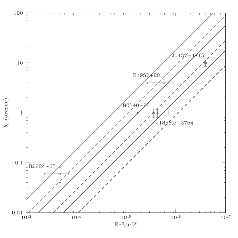
Figure 5: Scaling of the stand-off angle for H$\alpha$ bow shock nebulae with other observable parameters, as listed in Table 4.3. Circles mark radio pulsars and the cross marks RX J1856.5$-$3754, a radio-quiet NS. Lines of constant number density $n_{\rm A}=$ 0.01, 0.1, 1.0 cm^-3 are overplotted for inclination to the line of sight $i=90\arcdeg$ (thinnest to thickest solid lines) and $i=45\arcdeg$ (thinnest to thickest dashed lines).

The total H$\alpha$ flux from a bow shock nebula also scales with a combination of measured, observable and unknown parameters, as described by Eqns. 11 and 12. While $\dot{E}$, $\mu$, $D$ and $\theta_{0}$ are accessible to observation, the density $n_{\rm H}$ is unknown, and few a priori constraints exist on the neutral fraction $X$. Additionally, the scaling is a function of how the size of the bow shock depends on the velocity, parameterized as $\Delta\Omega\propto v_{\ast}^{2\beta}$, and we have argued that $\beta=1$.

The five bow shock nebulae with published H$\alpha$ flux values ($F_{\alpha}$) are plotted in Fig. 6 against two different combinations of observable and measured parameters, with $\beta=1$. While a correlation is apparent in the plot of $F_{\alpha}$ against $\theta_{0}^{2}\mu^{3}D^{3}$, it is worth noting that differences in the density and neutral fraction in the environment of each object and the different extinctions along each LOS are not accounted for in this plot, and neither is the projection effect for the velocity ($\sin^{3}i$), which differs for each bow shock. On the other hand, for $\beta=0$ (nebula size independent of velocity) and $\beta=0.5$, the points appear scattered with no discernible trend, favoring $\beta=1$ and $\Delta\Omega\propto v_{\ast}^{2}$. The two combinations of observables ($\theta_{0}^{2}\mu^{3}D^{3}$ and $\dot{E}\mu/D$) are related to each other through Eqn. 7, with differences in the medium density accounting for the relative scatter between the two plots.

Figure 6: Scaling of H$\alpha$ flux from bow shock nebulae with two different combinations of observable parameters, for $\dot{E}$ in erg s^-1, $\theta_{0}$ in arcsec, $\mu$ in mas yr^-1 and $D$ in kpc. Circles mark radio pulsars and the cross marks RX J1856.5$-$3754, a radio-quiet NS. The effects of the different inclinations to the LOS and the differing extinctions, densities and neutral fractions are not accounted for in these plots, and are responsible for the relative scatter between the two panels.

We note that there are two independent observed quantities ($\theta_{0}$ and $F_{\alpha}$) which depend on the measurable values for $\dot{E}$, $\mu$ and $D$ (as derived in §2). In principle, these can be combined to jointly constrain the unknown values of the density $n_{\rm H}$, neutral fraction $X$ and the inclination to the LOS. While current observations still lack the precision to produce meaningful constraints on all the unknown parameters at the same time, a parallax distance to PSR B2224+65 or a more precise measurement of the bow shock parameters for J0437$-$4715, for example, can be exploited in the future to obtain such constraints.

5.2 Bow Shocks at Radio/X-ray Wavelengths

As mentioned in §2.3, NS bow shocks consist of two shocked regions: an outer shock, where the ambient ISM undergoes collisional excitation and may emit in H$\alpha$, and an inner shocked region enclosing the relativistic NS wind, which may emit synchrotron radiation. No bow shocks have currently been detected in both H$\alpha$ and synchrotron radiation at radio wavelengths, although a faint extended X-ray counterpart may exist for the Guitar Nebula. It is possible that synchrotron-bright nebulae are observed only for younger NS, and radiation from the young NS or the parent supernova pre-ionizes the ISM, suppressing H$\alpha$ emission, or alternatively, that these younger NS are more likely to be found in superbubbles which have insignificant neutral fractions. Future observations should resolve this issue. Meanwhile, it is satisfying to recognize that the scaling argument for the stand-off radius developed for H$\alpha$ bow shocks can be applied to radio and X-ray detected synchrotron nebulae as well, in cases where a cometary morphology and a known radio pulsar indicate that a bow shock mechanism is at work.

There are several such radio pulsars which have associated plerionic bow shock nebulae at radio wavelengths, but not in H$\alpha$: for example, B1951+32 (Hester & Kulkarni, 1988), B1757$-$24 (the Duck, Frail & Kulkarni, 1991), B1853+01 (Frail et al., 1996) and B1643$-$43 (Giacani et al., 2001). Each of these has a clear association with a supernova remnant, attesting to the relative youth of the object. The best available parameters for these pulsars and the stand-off angles of the associated bow shocks (either quoted or estimated from the radio images) are listed in Table 5.2.

Table 3: Radio and X-ray Bow Shock Parameters

NS	SNR	D	V	$\log_{10}\dot{E}$	$\theta_{0}$	Refs.
		(kpc)	(km s-1)	(erg s-1)	(″)
B1643$-$43	G341.2+0.9	$6.9\pm 2.1$	$\sim 475$	35.55	$\leq 25$	1
B1757$-$24	G5.4$-$1.2	$4.6\pm 1.4$	$<550$	36.41	$1.5\pm 0.4$	2,3
B1853+01	W 44	$3.3\pm 1.0$	$\sim 375$	35.63	$\leq 1$	4
B1951+32	CTB 80	$2.4\pm 0.6$	$280\pm 80$	36.57	$3.0\pm 0.8$	5,6,7
B0906-49	$\cdots$	$6.6\pm 2.0$	$\sim 60$	35.69	$\leq 1$	8
B1823$-$13	$\cdots$	$4.1\pm 1.0$	$\cdots$	36.45	$\leq 40$	9
B1929+10	$\cdots$	$0.33\pm 0.01$	$163\pm 5$	33.59	$\cdots$	10,11,12
J0537$-$6910	N157B	$\sim 50$ (LMC)	$\sim 600$	38.68	$1.2\pm 0.4$	13
J0617.0+2221	IC 443	$1.5\pm 0.6$	$\sim 250$	$36\pm 0.3$	$8.5\pm 2.0$	14,†
The Mouse	G359.2$-$0.5?	$5.0\pm 1.0$	$\sim 180$	$36.3\pm 0.3$	$15\pm 4$	15,16,†

References. — (1) Giacani et al. (2001); (2) Frail & Kulkarni (1991); (3) $\mu<25$ mas yr^-1, Gaensler & Frail (2000); (4) Frail et al. (1996); (5) Strom (1987); (6) Migliazzo et al. (2002); (7) Hester & Kulkarni (1988); (8) Gaensler et al. (1998); (9) Finley, Srinivasan & Park (1996); (10) Yancopoulos, Hamilton & Helfand (1994); (11) Wang, Li & Begelman (1993); (12) Brisken (2001); (13) Wang et al. (2001); (14) Olbert et al. (2001); (15) Yusef-Zadeh & Bally (1987); (16) Predehl & Kulkarni (1995); (†: Not detected as a radio or X-ray pulsar.)

None of the listed pulsars has a parallax measurement, forcing us to rely on DM distances or estimates of the distance to the associated supernova remnant for $D$. The velocities are estimated from a recent proper motion measurement for B1951+32 (Migliazzo et al., 2002) and from the NS age and displacement from the supernova remnant center for B1853+01 and B1643$-$43. Ad hoc errors $\sim 25\%$ are assigned to the latter estimates, but it is worth emphasizing that they may be larger. For example, for B1757$-$24, a proper motion of 63–80 mas yr^-1 has been estimated from its spindown age and displacement from the alleged center of the remnant G5.4$-$1.2, but Gaensler & Frail (2000) find a $5\sigma$ upper limit $<25$ mas yr^-1 on its proper motion from interferometric observations. Only future interferometric measurements of the proper motions and parallaxes of these pulsars will reduce the large uncertainty associated with these estimates.

As before, the estimated stand-off angles (or limits) are plotted against a combination of observable parameters, and lines of constant density and inclination angle to the LOS are superimposed on the plot. It is immediately apparent that the large errors on the measurable parameters limit the useful constraints on the ISM density that can be extracted from the plot, and to illustrate the associated uncertainties, the location of B1757$-$24 using the erroneous proper motion estimate of 63–80 mas yr^-1 is also shown. However, it is reassuring that in spite of the large uncertainties, all the objects are consistent with physically plausible values of the ISM density.

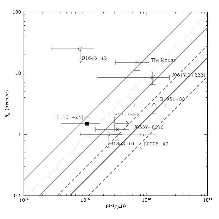
Figure 7: Scaling of stand-off angle with other observable parameters for X-ray and radio-detected bow shock nebulae, as listed in Table 5.2. Circles mark radio pulsars and crosses mark the X-ray pulsar J0537$-$6910, the radio-quiet NS CXOU J0617.0+2221, and the Mouse. The solid square shows B1757$-$24 when its proper motion is (erroneously) estimated from its spindown age and displacement from the alleged supernova remnant center, emphasizing the possible errors on this plot. Lines of constant number density $n_{\rm A}=$ 0.01, 0.1, 1.0 cm^-3 are overplotted, for inclination to the line of sight $i=90\arcdeg$ (thinnest to thickest solid lines) and $i=45\arcdeg$ (thinnest to thickest dashed lines).

An unusual radio nebula has been observed for B0906$-$49 (Gaensler et al., 1998), which appears to be a pulsar wind nebula generated by a slow-moving ($\sim 60$ km s^-1) pulsar and confined by the ISM with a stand-off angle $\leq 1\arcsec$. Using an analysis similar to this work, Gaensler et al. (1998) conclude that a dense ISM is required ($n_{\rm A}>2$ cm^-3).

Two other pulsars may have associated X-ray bow shock nebulae: B1823$-$13 and B1929+10. Both of these nebulae are ROSAT detections. For B1823$-$13, Finley, Srinivasan & Park (1996) suggest that the observed extended component may be either the associated supernova remnant for this young pulsar (spindown age $\sim 21$ kyr) or a bow shock nebula. If it is a bow shock nebula, the large scale size observed for the nebula ($\sim 40\arcsec$) implies either a low density medium or a low NS velocity. In the absence of a proper motion estimate, the situation cannot be resolved. For B1929+10, ROSAT data show a diffuse X-ray trail aligned with the pulsar proper motion, which has been explained as synchrotron radiation from a bow shock (Yancopoulos, Hamilton & Helfand, 1994; Wang, Li & Begelman, 1993). While an improved interferometric determination of the proper motion and parallax is available for this pulsar (Brisken, 2001), the stand-off angle cannot be determined from the ROSAT data. Future observations will complete the picture for these two pulsars.

In addition to synchrotron nebulae associated with known radio pulsars, there are two nebulae which are plausibly bow shocks associated with radio-quiet NS, the Mouse and the cometary nebula in IC 443, and a bow shock nebula associated with the X-ray pulsar J0537$-$6910, in the LMC.

G359.23$-$0.82 (the “Mouse”) was discovered in VLA observations by Yusef-Zadeh & Bally (1987). It appears to be a cometary wake, possibly emerging from the circular SNR G359.2$-$0.5. Though no associated radio pulsar was known, Predehl & Kulkarni (1995) found an X-ray counterpart, and suggested that the object was most likely a young NS bow shock, analogous to the one produced by B1951+32. They also estimate an $\dot{E}$ $\sim 10^{36.3}$ erg s^-1 from the ROSAT X-ray spectrum. Yusef-Zadeh & Bally (1987) estimate a velocity of $\sim 300$ km s^-1 for $D\approx 8.5$ kpc, which we scale down to 180 km s^-1 for $D\approx 5.0\pm 1.0$ kpc (Predehl & Kulkarni, 1995). For a stand-off angle $\sim 15\arcsec$, this implies an upper limit on the ISM density, $n_{\rm A}\lesssim 0.01$ cm^-3, which is fairly low. However, the previous caveats apply here, especially to the estimates of velocity and $\dot{E}$. A faint radio pulsar counterpart has recently been discovered (F. Camilio, private communication), opening up the possibility that these estimates may be improved in future.

A similar example is provided by the cometary nebula discovered by Olbert et al. (2001) in the supernova remnant IC 443. The NS producing this bow shock was detected by Chandra (CXOU J0617.0+2221), along with an X-ray counterpart to the radio synchrotron nebula. Based on the X-ray luminosity, $\dot{E}\sim 10^{36.3}$ erg s^-1. The distance to the associated SNR (and hence the NS) is $\sim 1.5$ kpc. From the bow shock morphology and the ratio of the NS velocity to the shock velocity in the SNR, Olbert et al. (2001) estimate a velocity of $250\pm 50$ km s^-1, independent of the distance.

J0537$-$6910 is a young Crab-like X-ray pulsar (16 ms period) in the LMC, associated with the SNR N157B, which was serendipitously discovered in RXTE observations (Marshall et al., 1998), but is not detected as a radio pulsar. Chandra observations show large scale diffuse emission, which is again consistent with a ram-pressure confined pulsar wind nebula (Wang et al., 2001). The pulsar has a measured spindown $\dot{E}=4.8\times 10^{38}$ erg s^-1, and a velocity $\sim 600$ km s^-1 estimated from its age and displacement from the SNR center. The estimated stand-off angle $=1\farcs 2\pm 0\farcs 4$ is consistent with the bow shock description.

The parameters for these objects are included in Table 5.2, and they are plotted in Fig. 7. The uncertainties are large, given the low confidence estimates of $D$, $\dot{E}$ and velocity. However, constraints on the density of the ISM can still be obtained, and their location on the plot suggests that the bow shock model is a suitable one for these objects.

6 DISCUSSION AND FUTURE WORK

Bow shock nebulae, produced by NS moving supersonically through the ISM, constitute unique probes of the energetic environment where NS relativistic winds interact with the surrounding ISM. In this work, we report multiwavelength observations of the Guitar Nebula, a spectacular H$\alpha$ bow shock nebula produced by a high velocity, modest $\dot{E}$ radio pulsar. High resolution HST observations show the detailed structure of the bright head of the nebula, confirming its limb-brightened nature and demonstrating the existence of a significant asymmetric component. The complex shape is best explained by the existence of a density gradient in the medium which is not aligned with the NS velocity vector.

A simple momentum conserving bow shock model is used to fit the HST observations and extract the stand-off angle $\theta_{0}$, as well as placing joint constraints on the inclination to the LOS, the density of the ambient medium, and the velocity and distance of the pulsar. While the low S/N ratio of the current HST image precludes a more detailed analysis, future HST data will provide more definitive constraints for some of these parameters.

The stand-off angle $\theta_{0}$ and the H$\alpha$ flux $F_{\alpha}$ scale with other measurable parameters ($\dot{E}$, $D$, $\mu$) and unknowns ($n_{\rm H}$, $X$). These scaling relationships are derived from the basic physics of the bow shock formation. Using the observations of the Guitar Nebula (described here) along with published parameters for the other known H$\alpha$ bow shocks, we confirm the scaling of $\theta_{0}$ with the other parameters for a diverse collection of nebulae, from simple canonical bow shocks to contorted shapes. The scaling relationship is used to derive upper limits on the density of the ambient medium, independent of the inclination of the bow shock to the LOS (which is hard to measure in a model-independent way). Additionally, the scaling of H$\alpha$ flux is demonstrated with different combinations of measurable parameters: while the relationship is not as constraining in this case, the observations conform to the expected scaling within the inherent uncertainties in the neutral fraction and extinction and the unknown density of the ambient medium.

We have also consolidated the available parameters for radio and X-ray bow shocks described in the literature, both for standard radio pulsars and radio-quiet or undetected NS. The stand-off angle appears to scale as expected for these objects as well. However, as described by Gaensler & Frail (2000) and illustrated by Fig. 7, the information available for these NS is inadequate, and has large margins of uncertainty. VLBI measurements of the parallaxes and proper motions of these objects will be essential for a clearer understanding of the physics of plerionic bow shock nebulae and their correlation with young NS and well-defined supernova remnants.

The observed anti-correlation of H$\alpha$ and plerionic radio emission from bow shocks is suggestive, though it needs to be confirmed in a larger sample of objects. Some young NS may be inside superbubbles created by previous supernovae, where the neutral fraction is insignificant. Pre-ionization of the medium, either by the young NS, or by the supernova in which it was born, may also suppress H$\alpha$ emission by reducing the enutral fraction, leading to the prediction that young NS with associated supernova remnants should not produce H$\alpha$ bowshocks. Conversely, if radiation from a young NS pre-ionizes the medium, H$\alpha$ bow shocks should only be associated with older NS. This would be consistent with the apparent drop off in the efficiency with which $\dot{E}$ is converted to radio emission in pulsar wind nebulae as a function of age (Gaensler et al., 2000).

Thus there are multiple avenues of future enquiry that promise to be fruitful. As the recently reported discovery of a bow shock nebula for B0740$-$28 demonstrates (Jones, Stappers & Gaensler, 2002), deep observations of suitably selected pulsars will probably result in the detection of more H$\alpha$ bow shocks, leading to constraints on the NS and ISM properties, as described in this work. Future radio and X-ray observations will also produce more such objects, and clarify the relationship between the NS age and environment and the type of bow shock emission. Additionally, further interferometric proper motions (and parallaxes, where possible) are required to produce firmer constraints on the properties of the ISM and the NS using known bow shock nebulae, while theoretical models of bow shock evolution can elucidate the differences in the behavior of bow shocks downstream from the stand-off region. It is also possible that old high-velocity neutron stars, including some born in the Galactic halo, may be identified through the serendipitous discovery of radio, X-ray or H$\alpha$ bow shock nebulae.

The Guitar Nebula, specifically, will continue to be of interest, both from a theoretical modeling perspective, and for observations of its evolution over time. Monitoring of the pulsar dispersion measure and changes in the shape of the head of the Guitar in multi-epoch high resolution observations will provide a unique perspective on the small-scale inhomogeneities in the interstellar medium.

References

- Arzoumanian, Chernoff & Cordes (2001) Arzoumanian, Z., Chernoff, D. F. & Cordes, J. M. 2001, ApJ, in press, astro-ph/0106159
- Baranov, Krasnobaev & Kulikovskii (1971) Baranov, V. B., Krasnobaev, K. V., & Kulikovskii, A. G. 1971, Soviet Phys.-Dokl., 15, 791
- Bell et al. (1995) Bell, J. F., Bailes, M., Manchester, R. N., Weisberg, J. M. & Lyne, A. G. 1995, ApJ, 440, L81
- Brisken (2001) Brisken, W. F., 2001, Ph.D. Thesis, Princeton University.
- Bucciantini & Bandiera (2001) Bucciantini, N. & Bandiera, R. 2001, A&A, 375, 1032
- Chevalier & Raymond (1978) Chevalier, R. A. & Raymond, J. C. 1978, ApJ, 225, L27
- Cordes & Chernoff (1998) Cordes, J. M. & Chernoff, D. F. 1998, ApJ, 505, 315
- Cordes, Romani & Lundgren (1993) Cordes, J. M., Romani, R. W. & Lundgren, S. C. 1993, Nature, 362, 133
- Deshpande, Ramachandran & Radhakrishnan (1999) Deshpande, A. A., Ramachandran, R., & Radhakrishnan, V. 1999, A&A, 351, 195
- Finley, Srinivasan & Park (1996) Finley, J. P., Srinivasan, R., & Park, S. 1996, ApJ, 466, 938
- Frail et al. (1996) Frail, D. A., Giacani, E. B., Goss, W. M., & Dubner, G. 1996, ApJ, 464, L165
- Frail & Kulkarni (1991) Frail, D. A. & Kulkarni, S. R. 1991, Nature, 352, 785
- Fruchter et al. (1992) Fruchter, A. S., Bookbinder, J., Garcia, M. R., & Bailyn, C. D. 1992, Nature, 359, 303
- Fruchter & Hook (2002) Fruchter, A. S. & Hook, R. N. 2002, PASP, 114, 144
- Gaensler & Frail (2000) Gaensler, B. M. & Frail, D. A. 2000, Nature, 406, 158
- Gaensler et al. (1998) Gaensler, B. M., Stappers, B. W., Frail, D. A., & Johnston, S. 1998, ApJ, 499, L69
- Gaensler et al. (2000) Gaensler, B. M., Stappers, B. W., Frail, D. A., Moffett, D. A., Johnston, S., & Chatterjee, S. 2000, MNRAS, 318, 58
- Giacani et al. (2001) Giacani, E. B., Frail, D. A., Goss, W. M., & Vieytes, M. 2001, AJ, 121, 3133
- Harrison, Lyne & Anderson (1993) Harrison, P. A., Lyne, A. G., & Anderson, B. 1993, MNRAS, 261, 113
- Hester & Kulkarni (1988) Hester, J. J. & Kulkarni, S. R. 1988, ApJ, 331, L121
- Högbom (1974) Högbom, J. A. 1974, A&AS, 15, 417
- Holtzman et al. (1995) Holtzman, J. A. et al. 1995, PASP, 107, 156
- Jones, Stappers & Gaensler (2002) Jones, D. H., Stappers, B. W. & Gaensler, B. M. 2002, A&A, submitted (astro-ph/—)
- Kaplan, van Kerkwijk & Anderson (2002) Kaplan, D. L., van Kerkwijk, M. H. & Anderson, J. 2002, ApJ, submitted (astro-ph/0111174)
- Kells et al. (1998) Kells, W., Dressler, A., Sivaramakrishnan, A., Carr, D., Koch, E., Epps, H., Hilyard, D., & Pardeilhan, G. 1998, PASP, 110, 1487
- Kulkarni & Hester (1988) Kulkarni, S. R. & Hester, J. J. 1988, Nature, 335, 801
- Lai, Chernoff & Cordes (2001) Lai, D., Chernoff, D. F., & Cordes, J. M. 2001, ApJ, 549, 1111
- Lyne & Lorimer (1994) Lyne, A. G. & Lorimer, D. R. 1994, Nature, 369, 127
- Markevitch et al. (2002) Markevitch, M., Gonzalez, A. H., David, L., Vikhlinin, A., Murray, S., Forman, W., Jones, C. & Tucker, W. 2002, ApJ, 567, L27
- Marshall et al. (1998) Marshall, F. E., Gotthelf, E. V., Zhang, W., Middleditch, J., & Wang, Q. D. 1998, ApJ, 499, L179
- McKee & Ostriker (1977) McKee, C. F. & Ostriker, J. P. 1977, ApJ, 218, 148.
- Migliazzo et al. (2002) Migliazzo, J. M., Gaensler, B. M., Backer, D. C., Stappers, B. W., van der Swaluw, E., & Strom, R. G. 2002, ApJ, 567, L141.
- Olbert et al. (2001) Olbert, C. M., Clearfield, C. R., Williams, N. E., Keohane, J. W., & Frail, D. A. 2001, ApJ, 554, L205
- Ostriker et al. (2001) Ostriker, E. C., Lee, C., Stone, J. M., & Mundy, L. G. 2001, ApJ, 557, 443
- Predehl & Kulkarni (1995) Predehl, P. & Kulkarni, S. R. 1995, A&A, 294, L29
- Ransom, Gaensler & Slane (2002) Ransom, S. M., Gaensler, B. M. & Slane, P. O. 2002, ApJ, submitted (astro-ph/0111339)
- Raymond (1991) Raymond, J. C. 1991, PASP, 103, 781
- Romani, Cordes & Yadigaroglu (1997) Romani, R. W., Cordes, J. M. & Yadigaroglu, I. -A. 1997, ApJ, 484, L137
- Spreiter & Stahara (1995) Spreiter, J. R. & Stahara, S. S. 1995, Advances in Space Research, 15, 433
- Spruit & Phinney (1998) Spruit, H. C. & Phinney, E. S. 1998, Nature, 393, 139
- Strom (1987) Strom, R. G. 1987, ApJ, 319, L103
- Taylor & Cordes (1993) Taylor, J. H. & Cordes, J. M. 1993, ApJ, 411, 674
- van Buren & McCray (1988) van Buren, D. & McCray, R. 1988, ApJ, 329, L93.
- van Buren & Mac Low (1992) van Buren, D. & Mac Low, M. 1992, ApJ, 394, 534
- van Kerkwijk & Kulkarni (2001) van Kerkwijk, M. H. & Kulkarni, S. R. 2001, A&A, 380, 221
- van Straten et al. (2001) van Straten, W., Bailes, M., Britton, M. C., Kulkarni, S. R., Anderson, S. B., Manchester, R. N. & Sarkissian, J. 2001, Nature, 412, 158.
- Walter (2001) Walter, F. M. 2001, ApJ, 549, 433
- Wilkin (1996) Wilkin, F. P. 1996, ApJ, 459, L31
- Wilkin (2000) Wilkin, F. P. 2000, ApJ, 532, 40
- Wang et al. (2001) Wang, Q. D., Gotthelf, E. V., Chu, Y.-H., & Dickel, J. R. 2001, ApJ, 559, 275
- Wang, Li & Begelman (1993) Wang, Q. D., Li, Z., & Begelman, M. C. 1993, Nature, 364, 127
- Wang & Loeb (2001) Wang, X. & Loeb, A. 2001, ApJ, 552, 49
- Yancopoulos, Hamilton & Helfand (1994) Yancopoulos, S., Hamilton, T. T., & Helfand, D. J. 1994, ApJ, 429, 832
- Yusef-Zadeh & Bally (1987) Yusef-Zadeh, F. & Bally, J. 1987, Nature, 330, 455