ON THE FORMATION OF MASSIVE STARS

Abstract

We calculate numerically the collapse of slowly rotating, non-magnetic, massive molecular clumps of masses 30 M_⊙, 60 M_⊙, and 120 M_⊙, which conceivably could lead to the formation of massive stars. Because radiative acceleration on dust grains plays a critical role in the clump’s dynamical evolution, we have improved the module for continuum radiation transfer in an existing 2D (axial symmetry assumed) radiation hydrodynamic code. In particular, rather than using “grey” dust opacities and “grey” radiation transfer, we calculate the dust’s wavelength-dependent absorption and emission simultaneously with the radiation density at each wavelength and the equilibrium temperatures of three grain components: amorphous carbon particles, silicates, and “dirty ice”-coated silicates. Because our simulations cannot spatially resolve the innermost regions of the molecular clump, however, we cannot distinguish between the formation of a dense central cluster or a single massive object. Furthermore, we cannot exclude significant mass loss from the central object(s) which may interact with the inflow into the central grid cell. Thus, with our basic assumption that all material in the innermost grid cell accretes onto a single object, we are only able to provide an upper limit to the mass of stars which could possibly be formed.

We introduce a semi-analytical scheme for augmenting existing evolutionary tracks of pre-main sequence protostars by including the effects of accretion. By considering an open outermost boundary, an arbitrary amount of material could, in principal, be accreted onto this central star. However, for the three cases considered (30 M_⊙, 60 M_⊙, and 120 M_⊙ originally within the computation grid), radiation acceleration limited the final masses to 31.6 M_⊙, 33.6 M_⊙, and 42.9 M_⊙, respectively, for wavelength-dependent radiation transfer and to 19.1 M_⊙, 20.1 M_⊙, and 22.9 M_⊙ for the corresponding simulations with grey radiation transfer. Our calculations demonstrate that massive stars can in principle be formed via accretion through a disk. The accretion rate onto the central source increases rapidly after one initial free-fall time and decreases monotonically afterwards. By enhancing the non-isotropic character of the radiation field the accretion disk reduces the effects of radiative acceleration in the radial direction — a process we denote the “flashlight effect”. The flashlight effect is further amplified in our case by including the effects of frequency dependent radiation transfer. We conclude with the warning that a careful treatment of radiation transfer is a mandatory requirement for realistic simulations of the formation of massive stars.

1 Introduction

Although massive stars play a critical role in the production of turbulent energy in the ISM, in the formation and destruction of molecular clouds, and ultimately in the dynamical and chemo-dynamical evolution of galaxies, our understanding of the sequence of events which leads to their formation is still rather limited. Because of their high luminosities we can expect: a) radiative acceleration will contribute significantly to the dynamical evolution during the formation process and b) the thermal evolution time scales of massive pre-main sequence objects will be extremely short. Thus, we cannot simply “scale up” theories of low mass star formation. Furthermore, OB stars form in clusters and associations; their mutual interactions via gravitational torques, powerful winds and ionizing radiation contribute further to the complexity of the problem.

Even though no massive disk has yet been directly observed around a main sequence massive star, it is likely that such disks are the natural consequence of the star formation process even in the high mass case. In their radio recombination maser studies and CO measurements Martin-Pintado et al. (1994) do find indirect evidence for both an ionized stellar wind and a neutral disk around MWC349. Moreover, several other high luminosity FIR sources — suspected embedded young OB stars — have powerful bipolar outflows associated with them (e.g., Eiroa et al. 1994; Shepherd et al. 2000). Such massive outflows are probably powered by disk accretion, and, similar to their low mass counterparts, the flow energetics appear to scale with the luminosity of the source (see Cabrit & Bertout 1992; Shepherd & Churchwell 1996; Richer et al. 2000).

The detailed structure and evolutionary history of massive circumstellar disks has important consequences with regard to the early evolution of these protostars. Disks provide a reservoir of material with specific angular momentum too large to be directly accreted by the central object. Only after angular momentum is transported outwards can this material contribute to the final mass of the star. The transition region disk-star will strongly influence the star’s photospheric appearance and how the star interacts with the disk. The relative high densities in these disks provide the environment for the further growth and evolution of dust grains, affecting the disk’s opacity and consequently its energetics and appearance. The disk can be expected to interact with stellar outflows and is likely to be directly responsible for the outflows associated with star formation.

Disks surrounding massive stars or disks associated with close companions to massive stars should be short-lived compared to their low mass counterparts. The UV environment within an OB cluster will lead to the photoevaporation of disks on a time scale of a few 10⁵ yr (Hollenbach, Yorke, & Johnstone 2000). Because this process operates on a time scale comparable to the formation of massive stars and is competitive to it, it is important to carefully model the transfer of radiation in the envelopes of accreting massive stars. Numerical tools capable of this task are lacking at present. We consider the present investigation as an important step in this direction.

2 The numerical model

We consider the simulation of the hydrodynamic collapse of a rotating molecular cloud clump, with wavelength-dependent radiation transfer, under the assumption of symmetry with respect to the rotation axis and the equatorial plane. Our code contains all of the basic features of the 2-D code described in detail by Yorke & Bodenheimer (1999; hereafter YB). In the following we shall discuss only the deviations from and enhancements to the YB code.

In addition to artificial viscosity for the treatment of shocks, physical viscosity has been implemented via an $\alpha$ prescription (Shakura & Sunyaev 1973): $\nu=\alpha c_{S}(r)H(r)$, where we have approximated the local disk scale height by $H(r)=c_{S}(r)/\Omega(r)$ ($\Omega$ is the angular velocity and $c_{S}$ is the sound speed). All components of the viscosity tensor are included, as previously implemented in 2-D disk models by Różyczka et al. (1994) and YB. Contrary to YB, who allowed $\alpha$ to vary in time in order to mimic the effects of tidal torques due to the growth of non-axisymmetric gravitational modes, the value for $\alpha=10^{-3}$ is was kept constant in space and time for all cases considered.

The details of this angular momentum transfer scheme — within certain limits — do not critically affect our results, however, because our central computational zone (where angular momentum transfer is presumably very critical) is so large. Test calculations with $\alpha=0.03$ yielded essentially the same results. By contrast, for $\alpha\leq 10^{-4}$ ring instabilities developed in the disk which led to a premature ending of the calculations. As discussed by Yorke, Bodenheimer, Laughlin (1995), who did not include the effects of angular momentum transfer (i.e., $\alpha=0$), these ring instabilities are unrealistic. Such a ring would be unstable on a very short (dynamical) time scale and the resulting clumps would exert tidal torques resulting in angular momentum transfer.

As in YB we utilize a series of hierarchically nested grids (Berger & Colella 1989; Yorke & Kaisig 1995). Whereas YB considered nesting levels of 6 and $60\times 60$ grids, allowing the innermost grid to be $\sim$1/2000 of the cloud radius, here we have considered nesting levels of 3 only and slightly larger grids ($64\times 64$). We assume constant density $\rho=\rho_{0}$ along the outermost radius $r_{\rm max}$ and allow material to enter into or exit from our computational grid $R^{2}+Z^{2}\leq r^{2}_{\rm max}$ ($R$ and $Z$ are the cylindrical coordinates), based on the sign of the radial component of the velocity. By contrast, YB assume a semi-permeable outer boundary at $r_{\rm max}$: Material with positive radial velocity can leave the computational grid but no mass was allowed to enter.

As in YB the boundary of the the innermost cell of our innermost grid is considered to be semi-permeable: Material can flow into this cell but cannot flow out of it. Material entering this cell is assumed to accrete onto a single central object. We realize that this “sink cell” procedure is a gross simplification of the physics in the innermost regions of our computational domain and a number of possibly important effects are being ignored, e.g. fragmentation and accretion of material onto multiple objects and the interaction of the accretion flow with powerful outflows. For the cases F30 and G30 (see section 3), for instance, our innermost cell is a cylinder of radius 40 AU and height 80 AU, whereas for the cases F120 and G120 the cell is larger by a factor of four. Although we cannot follow the mass flow within and possibly out of this cell, our simulations do provide upper limits to the amount of material which is available to be accreted by the central object: If radiative acceleration prevents the flow of material into the central sink cell, then the central object cannot accrete it.

2.1 Modeling the Central Star

In contrast to YB we consider a slightly more sophisticated treatment of the radius $R_{*}$, luminosity $L_{*}$, and effective temperature $T_{\rm eff}$ of the central object. Its mass $M_{*}$ is uniquely determined by integrating the mass flux into the center sink cell:

$$M_{*}=\int\dot{M}_{\rm*}\;dt\;.$$ (1)

We can express the total energy of the central core in terms of a “structure parameter” $\eta$:

$$E_{\rm tot}=-\eta{GM_{*}^{2}\over R_{*}}\;.$$ (2)

In principal, $\eta$, a parameter describing the compactness of the hydrostatic core, must be calculated by solving for the stellar structure of the accreting hydrostatic core. For polytropes of degree $n$, $\eta$ can be derived analytically (e.g. Kippenhahn & Weigert 1990):

$$\eta={3\over 10-2n}$$ (3)

A fully convective pre-main sequence protostar can be approximated by an $n=3/2$ polytrope and $\eta=3/7$. As the star approaches the main sequence, a greater proportion of it becomes radiative, its core becomes more compact, and $\eta$ increases.

For purposes of discussion we shall assume for the moment that $\eta=\eta(M_{*},R_{*})$ is a known function. In this case the intrinsic core luminosity $L_{*}$ (which does not include the contribution to the total luminosity emitted in the accretion shock front and dissipated within the disk) is given by:

$$L_{*} = L_{\rm nuc}-\dot{E}_{\rm tot}-\beta{GM_{*}\dot{M}_{*}\over R_{*}}$$ (4)

$$= L_{\rm nuc}-E_{\rm tot}\left[{\dot{\eta}\over\eta}+\left(2-{\beta\over\eta}\right){\dot{M}_{*}\over M_{*}}-{\dot{R}_{*}\over R_{*}}\right]$$ (5)

where $L_{\rm nuc}$ is the contribution from nuclear burning.

In the following we will assume that $\beta=1$: The material accreted by the star is being added ever so gently at its current radius $R_{*}$ and that this material adds negligible entropy to the star. For the total bolometric luminosity of a spherically accreting star, however, we must include the contribution of the potential energy of infalling material as it is dissipated on its way to the stellar surface:

$$L_{\rm bol}=L_{*}+L_{\rm acc}=L_{*}+\beta{GM_{*}\dot{M}_{*}\over R_{*}}$$ (6)

Equation 4 shows that for constant $L_{*}-L_{\rm nuc}$ the star should increase or decrease its radius due to mass accretion, depending on the sign of the coefficient of $\dot{M}_{*}/M_{*}$. Because $\beta\approx 1$ and $\eta\approx 3/7$ during the fully convective Hayashi phase, this coefficient is negative ($\approx-1/3$). Thus, mass accretion onto a fully convective star has a tendency to decrease the star’s radius, whereas close to the main sequence, where $\eta$ is closer to unity, mass accretion has a tendency to cause the star to bloat up (see Kippenhahn & Hofmeister 1977 for a more detailed discussion). In reality, the internal readjustment of the star after it has gained mass also affects the nuclear burning rate and thus has an effect on both radius and luminosity, depending on the magnitude of the mass accretion rate and the star’s current position in the Hertzsprung-Russell (HR) diagram.

A classical problem of the mathematical theory of stellar structure is the question of whether for stars of given fixed parameters, say chemical composition, mass, and radius, there exists one and only one solution of the basic structure equations. There is actually no mathematical basis for the so-called “Vogt-Russell” conjecture of uniqueness and indeed, multiple solutions for the same set of parameters have been found numerically in some cases (see discussion by Kippenhahn & Weigert 1990). However, for the rather simple cases considered here, spherically symmetric, quasi-hydrostatic homogeneous pre-main sequence and young main sequence stars, knowledge of the star’s mass and age at any given time does allow us to uniquely fix its position in the HR diagram, from which we can determine $L_{*}$, $T_{\rm eff}$, and $L_{\rm nuc}$.

For the pre-main sequence phase we shall account for deuterium burning only and use the following approximate expression:

$$L_{\rm nuc}=L_{D}\approx L_{0}(M_{*})\left[{\chi_{D}\over\chi_{D,0}}\right]\left[{R_{0}(M_{*})\over R}\right]^{p}\;,$$ (7)

where $L_{0}$ and $R_{0}$ are the equilibrium deuterium burning rate and equilibrium radius for a star of mass $M_{*}$ at its “birthline”, $\chi_{D,0}$ is the cosmic mass abundance of deuterium, and $\chi_{D}$ is the star’s net deuterium abundance. We have assumed $p=21$, which — because the star’s central density $\rho_{c}\propto R^{-3}$ — corresponds to $L_{D}\propto\rho_{c}^{7}$. This insures that a non-accreting star remains close to its birthline until a significant fraction of its deuterium is consumed.

Assuming instantaneous mixing during accretion, the deuterium mass fraction $\chi_{D}$ can be calculated from the following equation:

$${d\chi_{D}M_{*}\over dt}=\chi_{D,0}\dot{M}_{*}-\epsilon_{D}L_{D}\;,$$ (8)

where $\epsilon_{D}L_{D}$ is the rate of deuterium consumption due to deuterium burning ($\epsilon_{D}=1.76\times 10^{-19}\,{\rm s^{2}}\,cm^{-2}$ is a constant).

From equations 4 and 7 we can derive an expression for $\dot{R}_{*}$:

$${\dot{R}_{*}\over R_{*}} = \left[1-\eta_{R}\right]^{-1}\times$$ (10)

$$\left(\left[2-{\beta\over\eta}+\eta_{M}\right]{\dot{M}_{*}\over M_{*}}+{L_{*}-L_{\rm nuc}\over E_{\rm tot}}\right)$$

where

$$\eta_{R}=\left({\partial\ln\eta\over\partial\ln R}\right)_{M}\quad{\rm and}\quad\eta_{M}=\left({\partial\ln\eta\over\partial\ln M}\right)_{R}$$ (11)

From knowledge of $\eta(M_{*},R_{*})$, $L_{*}(M_{*},R_{*})$, $L_{0}(M_{*})$, and $R_{0}(M_{*})$ we approximate the pre-main sequence evolution of an accreting protostar by integrating equations 8 and 10 simultaneously.

How does one actually determine $\eta$ and $L_{*}$ from knowledge of $M_{*}$ and $R_{*}$? For the Hayashi phase we have used published pre-main sequence tracks for $L_{*}(M_{*},\tau)$, $R_{*}(M_{*},\tau)$ and set $\eta=3/7$. For the mass range 0.1 M_⊙ $\leq M_{*}\leq 2.5$ M_⊙ we use the evolutionary tracks of D’Antona & Mazzitelli (1994), which assume “CM convection” ($\alpha_{\rm ML}=2$) and Alexander + RI opacities ($Y=0.28$, $Z=0.019$). For 3 M_⊙ $\leq M_{*}\leq 15$ M_⊙ we use tracks published by Iben (1965). Both sets of tracks represent a series of stellar models which incorporate the detailed microphysics of convection and stellar atmospheres. For masses $M_{*}>15$ M_⊙ we have assumed that the evolutionary tracks for non-accreting stars are horizontal lines at the main sequence luminosity, similar to the 15 M_⊙ track (see Fig. 1), and the main sequence values of $R_{*}(M_{*})$ and $L_{*}(M_{*})$ were taken from Allen (1973).

As the contracting protostellar becomes radiative, $\eta$ increases. Once the star reaches the main sequence hydrogen burning commences and $\eta\approx$ const. We approximate $\eta$ during this phase by approximating the main sequence by polytropic models with the restriction that the main sequence value $\eta_{MS}\leq 1$. Obviously, this is a very rough approximation, but because we expect $\dot{\eta}\approx 0$ and $L_{*}\approx L_{\rm nuc}$ on the main sequence, we are not making a significant error. Our greatest error arises during the transition from $\eta=3/7$ (fully convective) to $\eta_{MS}$, where we have used interpolated values.

Of course, we could obtain a much better approximation to these physical parameters by solving the full set of radiation hydrodynamic equations for an accreting hydrostatic object. This, however, goes far beyond the scope of the present investigation. We merely wish to obtain more realistic approximations for $L_{*}$ and $R_{*}$ than those used by YB which were based on the pre-main sequence evolution of non-accreting low mass protostars. Because massive stars require at least one phase of high accretion rates, typically $\dot{M}_{*}\gtrsim 10^{-4}$ M_⊙ yr^-1, the effects of accretion on the evolution of $L_{*}$ and $R_{*}$ cannot be completely neglected. To illustrate this quantitatively we display the evolution of (proto-)stars accreting at given constant rates in the HR diagram (Fig. 1).

These tracks compare very well with published, more detailed calculations by Behrend & Maeder (2001) and by Meynet & Maeder (2000). Not only do the tracks lie slightly below the equilibrium deuterium burning “birthline” in all cases, but the qualitative effect of rapid accretion — namely to shift the tracks to even smaller radii below the “birthline” — occurs both in our simplified model and the above cited calculations. The reason for this is the negative sign of $2-\beta/\eta$ for fully convective stars. The tracks of our simplified model converge to the main sequence in a manner similar to those of the detailed calculations.

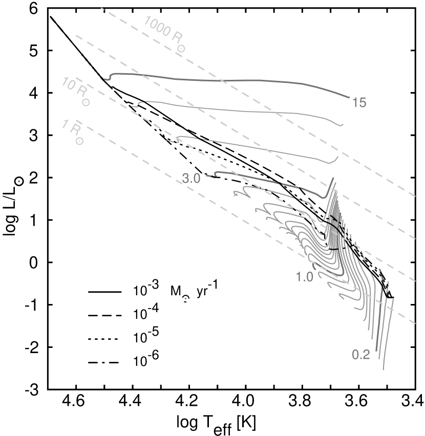
Figure 1: Evolutionary tracks of pre-main sequence stars accreting material at a constant rate as indicated. All accreting tracks begin at $M_{*}=0.1$ M_⊙ and $R_{*}=1$ R_⊙. The total bolometric luminosity, which includes contributions $L_{\rm acc}$ from the relaxation zone behind the accretion shock and emission from an accretion disk, is not shown. For comparison, the evolutionary tracks of non-accreting stars according to D’Antona & Mazzitelli (1994) and Iben (1965) are given (solid grey lines); the tracks for 0.2 M_⊙, 1.0 M_⊙, 3.0 M_⊙, and 15 M_⊙ are drawn slightly thicker.

There are some differences, however. Behrend & Maeder and Meynet & Maeder begin their tracks assuming a fully convective 0.7 M_⊙ star taken to be $7\times 10^{5}$ yr old, whereas we show here that the equilibrium deuterium-burning position at cosmic deuterium abundance is never reached via accretion for masses $M\lesssim 1$ M_⊙. If you add mass too quickly, the star’s radius is reduced as discussed above. If you add it too slowly (see $10^{-5}$ M_⊙ yr^-1 track in Fig. 1), a significant amount of the deuterium is consumed even before 0.7 M_⊙ has been accreted. Other differences are accountable by the different time dependent accretion rates.

We remind the reader that these tracks in the HR diagram do not reflect the actual observable bolometric luminosities of accreting protostars. Much of the accretion luminosity will be indistinguishable from the intrinsic luminosity of the star. For our hydrodynamic simulations we will include the effects of the accretion luminosity when discussing the star’s evolution within the HR diagram.

As in YB we add the accretion luminosity $L_{\rm acc}$ (Adams & Shu 1986) to the core’s intrinsic luminosity to obtain the total luminosity

$$L_{\rm tot}=L_{*}+\frac{3}{4}{GM_{*}\dot{M}_{*}\over R_{*}}$$ (12)

Equation 12 differs from equation 6 (for $\beta=1$), because approximately 1/4 of the total potential energy of the accreted material is dissipated within the disk and is already accounted for by our treatment of viscosity.

Finally, knowing $L_{\rm tot}$ and $R_{*}$ allows us to determine $T_{\rm eff}$ from:

$$L_{\rm tot}=4\pi\sigma_{\rm SB}R_{*}^{2}T_{\rm eff}^{4}\;.$$ (13)

$\sigma_{\rm SB}$ is the Stefan-Boltzmann radiation constant. When discussing the evolution of the central star in the HR diagram, we use $L_{*}$ rather than $L_{\rm tot}$ in equation 13.

2.2 The Opacity Model

The principal source of opacity is due to absorption and scattering by dust (cf. Yorke & Henning 1994). We have adopted the detailed frequency dependent grain model of Preibisch et al. (1993), which assumes a mixture of small amorphous carbon particles (for grain temperatures $T_{\rm aC}\leq 2000$ K) and “astrophysical silicate” grains (for temperatures $T_{\rm Si}\leq 1500$ K; c.f. Draine & Lee 1984). At grain temperatures $T_{\rm SiI}<125$ K the silicates are coated with a layer of “dirty” NH₃/H₂O ice, contaminated with 10% of the amorphous carbon particles. The grain sizes are assumed to follow an MRN power law $n(a)\sim a^{-3.5}$ (Mathis, Rumpl, & Nordsieck, 1977) in the size ranges 7nm $\leq a_{\rm aC}\leq 30$nm (carbon particles) and 40nm $\leq a_{\rm Si}\leq 1\mu$m (silicates). As evident in Figure 2, the specific extinction is strongly wavelength dependent.

Figure 2: Specific extinction $\sigma_{\nu}^{\rm ext}$ of the dust at temperatures below 125 K (aC + Silicate + Ice), between 125 K and 1500 K (aC + Silicate), and between 1500 K and 2000 K (aC).

For all our calculations we used 64 non-uniformly distributed frequency points between 5000  $\mu$m and 0.1  $\mu$m.

2.3 Modeling Radiation Transfer

A complete description of the radiation field requires knowledge of the radiation intensity $I_{\nu}({\bf x},\mbox{\bf\^{n}},t)$, where x indicates the position and n̂ the direction under consideration. Even assuming an axially symmetric configuration and plane symmetry with respect to the equatorial plane, $I_{\nu}$ is a function of 6 independent variables: frequency $\nu$, two spatial variables $(R,Z)$, two direction variables, say $(\theta,\phi)$, and time $t$. Solving the rather innocuous looking equation for radiation transfer

$$\frac{1}{c}\frac{dI\nu}{dt}+\nabla\cdot I_{\nu}=\kappa_{\nu}^{\rm ext}\,(S_{\nu}-I_{\nu})$$ (14)

($S_{\nu}$ is the source function and $\kappa_{\nu}^{\rm ext}=\sum_{i}\kappa_{\nu,i}^{\rm ext}$ is the net contribution to the extinction coefficient from all components “i”) together with the equations for hydrodynamics, energy balance, radiation equilibrium, and the Poisson equation for the gravitational potential becomes an formidable task with present day computers due to the vast number of computations which are necessary to obtain reasonable numerical resolution.

2.3.1 Flux-limited diffusion

The numerical problem can be greatly simplified by resorting to the flux-limited diffusion (FLD) approximation (see Yorke & Kaisig 1995, Levermore & Pomraning 1981). If we denote by $J_{\nu}$ and ${\bf H}_{\nu}$ the zeroth and first moments of the radiation field, respectively, where

$$J_{\nu}=\frac{1}{4\pi}\int I_{\nu}\,d\Omega\quad{\rm and}\quad{\bf H}_{\nu}=\frac{1}{4\pi}\int I_{\nu}\,\mbox{\bf\^{n}}\,d\Omega\;,$$ (15)

then the time independent form of the zeroth moment equation — obtained by integrating equation 14 over all directions — can be written:

$$\nabla\cdot{\bf H}_{\nu}=j_{\nu}+\sum_{i}\kappa_{\nu,i}^{\rm abs}\,[B_{\nu}(T_{i})-J_{\nu}]\;.$$ (16)

$\kappa_{\nu,i}^{\rm abs}$ is the absorption coefficient of grain type “i”, $T_{i}$ is its temperature, $B_{\nu}(T)$ is the Planck function, $j_{\nu}$ is the contribution to the emissivity from internal sources other than dust emission. The next higher order moment equation, obtained by multiplying the time independent form of equation 14 by n̂ and then integrating over all directions, would contain terms involving the second moment of the radiation field.

The FLD approximation is a procedure for closing this series of moment equations by approximating the second moment in terms of the zeroth and first moments, utilizing knowledge of the opacity distribution:

$${\bf H}_{\nu}=-\frac{\lambda_{\nu}}{\omega_{\nu}\kappa_{\nu}^{\rm ext}}\nabla J_{\nu}\;.$$ (17)

The effective albedo $\omega_{\nu}$ and the flux limiter $\lambda_{\nu}$ are defined as ($\kappa_{\nu,i}^{\rm sca}$ is the scattering coefficient for grain type “i”):

$$\omega_{\nu}=\sum_{i}\frac{\kappa_{\nu,i}^{\rm abs}B_{\nu}(T_{i})+\kappa_{\nu,i}^{\rm sca}J_{\nu}}{\kappa_{\nu,i}^{\rm ext}J_{\nu}}$$ (18)

$$\lambda_{\nu}=\frac{1}{d}\left(\coth d-\frac{1}{d}\right)\quad{\rm with}\quad d=\frac{|\nabla J_{\nu}|}{\kappa_{\nu}^{\rm ext}\omega_{\nu}J_{\nu}}$$ (19)

In the limits of high opacity or low opacity, the FLD approximation asymptotically approaches the diffusion limit or the free-streaming limit, respectively, as expected.

The equations 16 and 17 have to be solved for all frequencies simultaneously with the condition for radiative equilibrium of each of the absorbing species:

$$\int\kappa_{\nu,i}^{\rm abs}\left[B_{\nu}(T_{i})-J_{\nu}\right]\,d\nu=0\;.$$ (20)

When considering “grey” radiation transfer as YB did, this condition can be put into tabular form (for rapid look-up):

$$T_{i}={\cal T}_{i}(J)\quad{\rm with}\quad J=\int J_{\nu}\;d\nu\;.$$ (21)

2.3.2 Finite Difference Equations

Following a “staggered mesh” discretization philosophy for converting partial derivatives into finite differences, we define $J_{\nu}$ at the cell centers of an $(R_{j},Z_{k})$ cylindrical grid and the vector ${\bf H_{\nu}}=(H_{\nu,R},H_{\nu,Z})$ at the centers of cell boundaries. Combining the equations 16 and 17 we obtain a diffusion equation

$$\nabla\cdot\left({\cal D}_{\nu}\nabla J_{\nu}\right)=j_{\nu}+\sum_{i}\kappa_{\nu,i}^{\rm abs}\left[J_{\nu}-B_{\nu}(T_{i})\right]\;.$$ (22)

The discretized form of this FLD equation can be expressed as a matrix equation:

$${\cal A}_{\nu}{\bf J}_{\nu}=\epsilon_{\nu}({\bf T})\;,$$ (23)

where the vector ${\bf J}_{\nu}$ represents the solution for the zeroth moment and $\epsilon_{\nu}({\bf T})$ the dust temperature dependent components for the source terms at all grid centers. We employ an equidistant $(R_{j},Z_{k})$ grid at each level of nesting and, while utilizing a 5-point discretization scheme,

$$a_{l,j,k}^{01}J_{l,j-1,k}+a_{l,j,k}^{10}J_{l,j,k-1}+a_{l,j,k}^{11}J_{l,j,k}$$ (24)

$$+a_{l,j,k}^{21}J_{l,j+1,k}+a_{l,j,k}^{12}J_{l,j,k+1}$$ (25)

$$=j_{l,j,k}-\sum_{i}\kappa_{l,i,j,k}^{\rm abs}B_{l}(T_{i,j,k})\;,$$ (26)

insure by proper centering that our finite difference equation 23 is accurate to second order ${\cal O}(h^{2})$ of the grid spacing $h=R_{j+1}-R_{j}=Z_{k+1}-Z_{k}$. In equation 24 we have used the subscript $l$ for frequency and $i$ for grain type.

Note that ${\cal A}_{\nu}$ is an implicit function of ${\bf J}_{\nu}$. Each element of ${\cal A}_{\nu}$ for frequency $\nu$ at a grid cell $(j,k)$ contains, with proper centering, $J_{\nu^{\prime}}$ dependencies for all frequencies $\nu^{\prime}$ and extending beyond the 5-point discretization star of grid cells $(j,k)$ and $(j\pm 1,k\pm 1)$. As evidenced by equation 20 the right hand side of equation 24 is also an implicit function of ${\bf J}_{\nu}$. The fact that we must find a new solution iteratively on each nested grid for each hydrodynamic time step places strong demands on our solution algorithm.

2.3.3 Boundary conditions

Boundary conditions are required for each level of nested grids. For each grid cell $(R_{j},Z_{k})$ on the outermost grid which satisfies the condition $R_{j}^{2}+Z_{k}^{2}\geq r^{2}_{\rm max}$ we specify $J_{\nu}=w\,B_{\nu}(T_{\rm out})$, where $T_{\rm out}$ is the color temperature of an external isotropic radiation field and $w$ is the radiation dilution factor. For all cases considered here we choose $w=1$ and $T_{\rm out}=20\,$K. Along the outer edges of interior (fine) grids we use the interpolated value of $J_{\nu}$ from the next (coarser) grid level. Additional boundary conditions along the rotation axis and equatorial plane result from the assumed symmetry.

Within the innermost central grid cell of each level of nested grids we treat the central star as an additional internal source of emissivity and define $j_{\nu}$ (see equation 16) accordingly:

$$j_{\nu}={\pi R_{*}^{2}\over 2\pi R_{1}^{2}Z_{1}}B_{\nu}(T_{\rm eff})~{},$$ (27)

where $R_{1}$ and $Z_{1}$ are the radial extent and height of the central cell.

2.4 Solution algorithms

Because of the necessity of solving equations 20 and 22 repeatedly on several grids during the course of hydrodynamic evolution, it was imperative to make this module fast and robust. Several promising algorithms which rely on fine-tuning adjustable parameters had to be abandoned, because a wide range of problem classes (optically thin, optically thick, strong density gradients, emission-dominated, scattering-dominated, etc.) occurred, which were not well suited to a single set of parameters. We were able to make vast improvements with respect to the iterative procedures used by Sonnhalter et al. (1995), who solved these same frequency dependent equations for a few selected density configurations. We sometimes sacrificed robustness (but never accuracy) for speed but automatically fell back to slower and more robust iterative schemes when the “faster” algorithms failed to converge. We feel it is useful to discuss our “failures” as well as our “successes” in our endeavor to improve the speed of our frequency dependent radiation transfer module.

2.4.1 Temperature determination

In analogy to the transfer of line radiation in stellar atmospheres we consider the method of approximate $\Lambda$ operators (see e.g. Cannon 1973a,b and Scharmer 1981). Rewriting equation 23 with the operator $\Lambda={\cal A}^{-1}$, we find the formal solution:

$${\bf J}_{\nu}=\Lambda_{\nu}\epsilon_{\nu}({\bf T})$$ (28)

A simple $\Lambda$-iteration would entail calculating ${\bf T}^{\rm old}$ and thus $\epsilon_{\nu}({\bf T}^{\rm old})$ from ${\bf J}_{\nu}^{\rm old}$ using equation 20. From this, a new, improved estimate for ${\bf J}_{\nu}$ can be calculated: ${\bf J}_{\nu}^{\rm new}=\Lambda_{\nu}\epsilon_{\nu}({\bf T}^{\rm old}$). Replacing ${\bf J}_{\nu}^{\rm old}$ by ${\bf J}_{\nu}^{\rm new}$ and repeating this procedure several times may or may not (usually not) quickly converge to the equilibrium values for ${\bf T}$ and ${\bf J}_{\nu}$ satisfying equation 28. This procedure is labelled “$\Lambda$” in Table 1.

In order to improve convergence we consider an appropriate approximation $\Lambda_{\nu}^{*}$ to our operator $\Lambda_{\nu}$. Rather than using ${\bf J}_{\nu}^{\rm old}$ in equation 20 we substitute the expression

$${\bf J}_{\nu}^{\rm new}={\bf J}_{\nu}^{\rm old}+\Lambda_{\nu}^{*}\left[\epsilon_{\nu}({\bf T}^{\rm new})-\epsilon_{\nu}({\bf T}^{\rm old})\right]$$ (29)

to obtain the equilibrium conditions for each grain component “$i$”:

$$\int\kappa_{\nu,i}^{\rm abs}\left[B_{\nu}(T_{i}^{\rm new})-\Lambda_{\nu}^{*}\epsilon_{\nu}({\bf T}^{\rm new})\right]\,d\nu$$ (30)

$$=\int\kappa_{\nu,i}^{\rm abs}\left[{\bf J}_{\nu}^{\rm old}-\Lambda_{\nu}^{*}\epsilon_{\nu}({\bf T}^{\rm old})\right]\,d\nu\;,$$ (31)

which can be rewritten in the form ${\bf G}({\bf T}^{\rm new})=0$. The solution vector ${\bf T}^{\rm new}$ can be obtained by solving equation 30 using a multidimensional Newton-Raphson procedure.

Our approximate $\Lambda$ iteration procedure entails alternatively solving equation 30 for ${\bf T}^{\rm new}$ and equation 23 for ${\bf J}_{\nu}^{\rm new}$.

There are many possibilities for $\Lambda_{\nu}^{*}$, and much effort has been invested in order to optimize its construction. Generally speaking, the choice of a particular $\Lambda_{\nu}^{*}$ is based on performance during numerical experimentation and varies from problem to problem. Following this heuristic approach we considered several different approximate operators and compared their convergence properties with the simple $\Lambda$ iteration. Our test cases were the first 20 time steps of two single grid collapse calculations with a) $13\times 13$, b) $128\times 128$ grid cells, and c) the results of time step 2900 of the 30 M_⊙ case discussed in section 4. For these test calculations we utilized the most efficient procedure for solving equation 23 for ${\bf J}_{\nu}^{\rm new}$ (discussed below). The average number of $\Lambda$ iterations necessary for each approximate operator and for each test case is given in Table 1.

Table 1: TEMPERATURE ITERATIONS

	a	b	c
procedure	13x13	128x128	3*64x64
$\Lambda$	10.1	16.4	57.8
core-wing	10.9	—	—
diagonal	4.3	10.1	$>100$
acc-diag	4.35	—	—
$\Lambda^{S}$	—	—	10.2

Our approximate “core-wing” operator is constructed in analogy to the “core-wing” $\Lambda$ operator of Scharmer (1981) which takes into account that lines are often optically thin in the wings and optically thick in the line’s core. The analogy with a more or less monotonously decreasing (or increasing) continuum absorption coefficient is to assume a threshold value for which the dusty material becomes optically thin. We conducted several numerical experiments with different threshold values but found little improvement in comparison to the simple $\Lambda$ iteration procedure.

Defining $\Lambda_{\nu}^{\rm diag}={\it diag}({\cal A})^{-1}$ resulted in improved convergence behavior. Use of additional accelerator terms as outlined by Auer (1987), however, did not always lead to further improvement. Our best convergence results were attained with the $\Lambda_{\nu}^{S}$ operator constructed as follows. We first approximate $J_{l,j,k}$ by using the diagonal operator $\Lambda_{\nu}^{\rm diag}$ in equation 28:

$$J_{l,j,k}^{*}({\bf T})=\frac{j_{l,j,k}-\sum_{i}\kappa_{l,i,j,k}^{\rm abs}B_{l}(T_{i,j,k})}{a_{j,k}^{11}}\;.$$ (32)

This approximation is used for the off-diagonal terms in equation 24 to obtain:

$$J_{l,j,k}=({a_{l,j,k}^{11}})^{-1}\Bigl{[}j_{l,j,k}-\sum_{i}\kappa_{l,i,j,k}^{\rm abs}B_{l}(T_{i,j,k})$$ (33)

$$-a_{l,j,k}^{01}J_{l,j-1,k}^{*}({\bf T})-a_{l,j,k}^{21}J_{l,j+1,k}^{*}({\bf T})$$ (34)

$$\quad-a_{l,j,k}^{10}J_{l,j,k-1}^{*}({\bf T})-a_{l,j,k}^{12}J_{l,j,k+1}^{*}({\bf T})\Bigr{]}\;.$$ (35)

Because the right hand side depends only on known quantities and the temperatures ${\bf T}$ this corresponds to the operator equation

$${\bf J}_{\nu}=\Lambda_{\nu}^{S}\epsilon_{\nu}({\bf T})\;.$$ (36)

Use of $\Lambda_{\nu}^{S}$ sometimes leads to oscillations during the iterations which we are able to damp by interjecting simple $\Lambda$ iterations.

Occasionally, the Newton-Raphson iteration procedure used for solving equation 30 did not converge. For these special cases we had to abandon our approximate $\Lambda$ iterations in favor of the following more robust but much more CPU intensive procedure. If we denote by $\tilde{T}_{i}$ our (inaccurate) estimate of $T_{i}$ then a temperature correction $\Delta T_{i}$ can be determined from:

$$\Delta T_{i}=\frac{\sum_{\mu}w_{\mu}\kappa_{\mu,i}^{\rm abs}\left[J_{\mu}-B_{\mu}(\tilde{T}_{i})\right]}{\sum_{\mu}w_{\mu}\kappa_{\mu,i}^{\rm abs}dB_{\mu}/dT|_{T=\tilde{T}_{i}}}\;,$$ (37)

where we have replaced the frequency integration by a weighted sum with the weights $w_{\mu}$. By substituting $B_{\nu}(\tilde{T}_{i})+dB_{\nu}/dT|_{T=\tilde{T}_{i}}\Delta T_{i}$ for $B_{\nu}(T_{i})$ on the right hand side of equation 22 and replacing $\Delta T_{i}$ by the expression given in equation 37 we find a modified FLD equation:

$$\nabla\cdot\left({\cal D}_{\nu}\nabla J_{\nu}\right)=j_{\nu}+\sum_{i}\kappa_{\nu,i}^{\rm abs}\Bigl{(}J_{\nu}-B_{\nu}(\tilde{T}_{i})$$ (38)

$$-\frac{dB_{\nu}}{dT}\bigr{|}_{T=\tilde{T}_{i}}\frac{\sum_{\mu}w_{\mu}\kappa_{\mu,i}^{\rm abs}\left[J_{\mu}-B_{\mu}(\tilde{T}_{i})\right]}{\sum_{\mu}w_{\mu}\kappa_{\mu,i}^{\rm abs}dB_{\mu}/dT|_{T=\tilde{T}_{i}}}\Bigr{)}\;,$$ (39)

which can be expressed in matrix form as

$${\cal A}_{\nu}{\bf J}_{\nu}+\sum_{\mu}{\cal C}_{\nu\mu}{\bf J}_{\mu}=\chi_{\nu}({\bf T})\;.$$ (40)

The iteration procedure now consists of alternatively solving equations 37 and 40 until convergence. Because this alternative procedure is more CPU-intensive than the approximate $\Lambda$ iterations described above, it is only used when absolutely necessary.

2.4.2 Solution of the partial differential equations

The partial differential equations 22 or 38 have to be solved repeatedly for each hydrodynamic time step and for each frequency. The coefficients ${\cal D}_{\nu}$, $\kappa_{\nu,i}^{\rm abs}$ and $\epsilon_{\nu}$ depend on frequency and position and vary from time step to time step. The relative importance of individual terms can vary strongly from position to position and with time: i.e. both

$$\bigl{|}\nabla\cdot{\cal D}_{\nu}\nabla J_{\nu}\bigr{|}\gg\Bigl{|}j_{\nu}+\sum_{i}\kappa_{\nu,i}^{\rm abs}[J_{\nu}-B_{\nu}(T_{i})]\Bigr{|}$$

and

$$\bigl{|}\nabla\cdot{\cal D}_{\nu}\nabla J_{\nu}\bigr{|}\ll\Bigl{|}j_{\nu}+\sum_{i}\kappa_{\nu,i}^{\rm abs}[J_{\nu}-B_{\nu}(T_{i})]\Bigr{|}$$

occur.

In addition to the “alternating direction implicit” procedure (ADI) we considered the multi-grid scheme “full approximation storage” (FAS), “successive over-relaxation” (SOR) and its special case by Gauss-Seidel (GS), the method of “quasi-minimal residues” (QMR), and bicgstab(2), an improvement on the “Bi-CGSTAB” algorithm (“Bi-CGSTAB” combines the advantages of GMRES and Bi-CG). More information on the ADI, FAS, SOR, and GS procedures can be found in Press et al. (1992). Our variant of the QMR procedure is described by Bücker & Sauren (1996) and the bicgstab(2) method is described in full detail by Sleijpen & Fokkema (1993).

Figure 3: Convergence properties of four versions of the partial differential equation solver for equation 22 are shown at three wavelengths: 435 nm (high optical depth), 21 $\mu$m (optical depth of order unity), and 1100 $\mu$m (small optical depth). The “residual” is the Euclidean norm of $\left|{\cal A}_{\nu}{\bf J}_{\nu}-\epsilon_{\nu}({\bf T})\right|$ over the entire grid.

Our standard test problem was constructed from the density distribution calculated by Yorke, Bodenheimer, Laughlin (1995) for the case of a slowly rotating 10 M_⊙ molecular clump, 7074 years after the beginning of collapse (see their Fig. 4). The density was remapped onto a single $66\times 66$ grid. Assuming a central luminosity of 100 L_⊙ and constant dust temperature ($T_{i}=20\,$K) as starting values, we constructed an initial model by iterating equation 22 until convergence using SOR, subsequently solving for the corrected temperatures using equation 20. The time required for this first iterative step was not included in our comparison. Each procedure was coded in fortran90 and optimized for vector processing; a single processor of a CRAY T90 was used for the comparison calculations, the results of which are shown in Figure 3 and Table 2 for ADI, QMR, bicgstab(2), and GS.

Table 2: CPU TIME NECESSARY FOR CONVERGENCE

procedure	$1100\,\mu$m	435 nm
ADI	2.12	$>600$
GS	3.98	14.30
QMR	2.17	2.03
bicgstab(2)	1.15	1.38

We first note that the ADI procedure used by Sonnhalter et al. (1995) did not converge for several frequencies for our test problem; the residual in the central cell remained constant after a few iterations. This problem was alleviated by resorting to SOR; the most robust variant used an over-relaxation parameter $\omega=1$, reducing SOR to the GS procedure. GS iterations resulted in steadily (but slowly) decreasing residuals. QMR and bicgstab(2) required the fewest number of iterations to reach convergence, but because of their complexity, it is not immediately apparent that these procedures would also require the least amount of CPU time. As shown in Table 2 bicgstab(2) did indeed prove to be the most efficient partial differential equation solver. It was used for our numerical simulations discussed in section 4. Every variant of FAS we attempted diverged for our test problem and the method was quickly abandoned.

3 Initial conditions

In spite of recent observational and theoretical progress, the initial conditions for protostellar collapse are still poorly known. Whereas it is clear that the formation of massive stars require high masses, neither the average temperatures nor the sizes and density distributions of those molecular clumps on the brink of forming massive stars are especially well known (Stahler, Palla, & Ho 2000).

Because we are investigating whether massive stars can form by accretion, comparable to our current understanding of low mass star formation rather than by coalescence of lower mass hydrostatic components or stellar coalescence (see e.g. Bonnell, Bate, & Zinnecker 1998), we will adopt for our initial conditions a scaled-up version of the initial configuration expected for the formation of low mass stars (see e.g. Williams, Blitz, & McKee 2000 or André, Ward-Thompson, & Barsony 2000 for extensive reviews): clump sizes are a fraction of a pc, temperatures lie in the range 10–30 K (we adopt $T_{0}=20\,$K), and the clumps are density-peaked towards the center (typically, $\rho\propto r^{-p}$, where $p\approx 1-2$). Because high mass star formation is an extremely rare event, we do not restrict ourselves to clump masses which are one or two Jeans masses only. We adopt a thermal to gravitational binding energy ratio of $E_{T}/|E_{G}|=0.05$, corresponding to about 10 Jeans masses. However, because gravity always dominated thermal pressure forces in our domain of integration, we expect no significant evolutionary differences as long as $T_{0}\lesssim 100\,$K ($M\gtrsim 2$ Jeans masses).

Table 3: INITIAL CONDITIONS FOR COLLAPSE

frequency-dependent	F30	F60	F120
grey cases	G30	G60	G120
Mass [M⊙]	30	60	120
Radius [pc]	0.05	0.1	0.2
$T_{0}$ [K]	20	20	20
$\Omega_{0}$ [10-13 s-1]	5	5	5
$\rho_{0}$ [$10^{-20}$ g cm-3]	1	1	1
$\left<n_{H}\right>$ [105 cm-3]	23	5.8	1.5
$E_{T}/|E_{G}|$	0.05	0.05	0.05
$E_{\rm rot}/|E_{G}|$	0.023	0.094	0.374
$t_{\rm ff}$ [$10^{3}$ yr]	32	65	129

The initial configuration is summarized in Table 3. We begin with a rotating ($\Omega=5\times 10^{-13}\,$s^-1) density configuration $\rho\propto r^{-2}$. This power law dependence corresponds to that expected in the central regions of magnetically supported, slowly contracting, slowly-rotating clouds (Mouschovias 1990; Tomisaka, Ikeuchi, & Nakamura 1990; Lizano & Shu 1989; Crutcher et al. 1994). Probably the best measured pre-collapse core, L1689B, has a somewhat flatter central region ($R\lesssim 4000$ AU) with $\rho\propto r^{-0.4}$ or $\rho\propto r^{-1.2}$, depending on geometric and temperature assumptions (André, Ward-Thompson, & Motte 1996). Outside 4000 AU the density decreases as $\rho\propto r^{-2}$. By contrast, Motte, André, & Neri (1998) find $\rho\propto r^{-2}$ density profiles in 10 compact pre-collapse cores in the $\rho$ Oph region, which they were able to resolve down to $\sim$140 AU.

In spite of the fact that the radial dependence of density in pre-collapse cores is observationally ill-constrained, especially for the high mass case, we have restricted ourselves to an initial $\rho\propto r^{-2}$ density configuration, corresponding to that of a “singular isothermal sphere”, which has been used for many years to model the formation of low mass stars. This allows direct comparision with the results of analogous collapse calculations. During the course of evolution, however, rotation, thermal forces at the outermost radius, and radiation forces quickly modify this initial density distribution. Moreover, in contrast to similarity solutions that rely on the assumption of a singular isothermal sphere our clumps are initially at rest. The mass accretion rates are thus not fixed, but rather a result of the radiation hydrodyanmic calculations.

For the cases F120 and G120 the rotational velocity at the equator and $r_{\rm max}$ exceeded the escape velocity. Thus, about 7.3 M_⊙ of the original 120 M_⊙ in the cloud was not bound initially.

4 Results

4.1 Evolution of the Central (Proto-)Star

We have implicitly assumed that all material flowing into the central zone is accreted onto a single object. Its mass is known from integrating the mass accretion rate $\dot{M}_{*}$ over time; its luminosity and effective temperature are modeled according to the procedure described in section 2.1. In Fig. 4 we display the evolution of the total and accretion luminosities for the frequency-dependent “F” sequences.

Figure 4: Total luminosity (solid lines) and accretion luminosity (dashed lines) for the frequency-dependent “F” sequences

Considering the fact that the initial free-fall times double from case F30 to F60 and from F60 to F120, the initial rapid rise of luminosity — due to the emission from an accretion shock surrounding the central star — appears similar for all three cases. This is not too surprising, because neither rotation nor radiation has an important influence during these early phases; the flow is dominated by gravity. After several thousand years, the energy released within the accretion shock front is not the dominant source of luminosity. Adding material onto the central star at the very high rates considered here causes it to bloat up to radii exceeding the deuterium burning limit (see Fig. 5). Note that there is very little difference of the evolution within the HR diagram of these three cases. Indeed, except for a “shift” in time and the maximum mass attained in each simulation, the growth of mass within the central computational zone was remarkably similar (c.f. Fig. 6). The rate of mass accretion rises sharply within a few thousand years, reaches a maximum value $\sim 2\times 10^{-3}$ M_⊙ yr^-1.

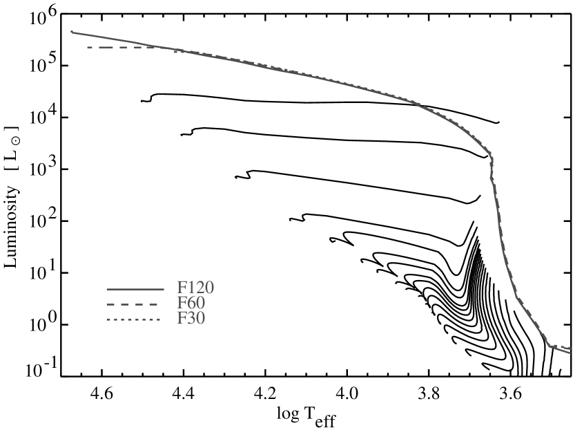
Figure 5: Evolution of the central (proto-)stars for the frequency-dependent “F” sequences in the HR diagram. The luminosity contribution $L_{\rm acc}$ from the relaxation zone behind the accretion shock has been included. For comparison, the evolutionary tracks of non-accreting stars has been given (c.f. Fig. 1).

Comparing these tracks with those published by Behrend & Maeder (2001) by Meynet & Maeder (2000), we note that our tracks lie significantly higher in the HR diagram (larger radii, larger luminosity, but slightly lower $T_{\rm eff}$ for equivalent masses) and cross the main sequence at a somewhat higher luminosity by about 0.5 to 0.8 dex. This is not too surprising, because our luminosity includes 3/4 of the accretion luminosity (see equation 12) and our accretion rate varied in time according to the results of hydrodynamic calculations (see Fig. 6 and Fig. 7). By contrast, Behrend & Maeder assumed a given accretion rate onto the star based on observations of outflows $\dot{M}_{*}=\max(10^{-5}\;{\rm M}_{\odot}\;{\rm yr}^{-1},\tilde{f}\,\dot{M}_{\rm out})$, where $\tilde{f}$ was chosen to lie between 0.3 and 0.5. For outflow mass loss $\dot{M}_{\rm out}$ the authors used the observed relation between the outflow mass rates and the stellar bolometric luminosities in ultracompact HII regions found by Churchwell (1998) and confirmed by Henning et al. (2000). Meynet & Maeder used the formula $\dot{M}_{*}=10^{-5}\;{\rm M}_{\odot}\;{\rm yr}^{-1}\max(1,M_{*}/{\rm M}_{\odot})^{1.5}$.

The formulae assumed by Behrend & Maeder and by Meynet & Maeder result in higher accretion times (lower average accretion rates) and a shift of the phase of extremely high accretion rates to later evolutionary times, compared to what we find in our collapse calculations. At the high mass end, however, the evolution of the star is similar; the tracks follow closely along the main sequence in spite of high mass accretion rates.

Figure 6: Evolution of the central (proto-)stars’ masses for the frequency-dependent “F” sequences. After an initial delay the mass accretion rates rise rapidly to comparable values (given by the slope of the curves) and fall off rapidly as radiative effects inhibit further accretion (see also Fig. 7).

The growth of mass in the central computational zone was governed by the relative importance of centrifugal, radiative, and gravitative forces in the molecular clump. For the six cases calculated we found that the detailed treatment of radiation transfer strongly influenced the clump’s evolution. In general, the accretion rate increased sharply after about one free-fall time and then decreases. To exemplify this we display the growth of central mass and the time dependence of the accretion rate for the frequency-dependent case F60 and for the grey case G60 in Fig. 7. Assuming grey radiation transfer, in infall of material into the central regions of the molecular clump is strongly hampered after about 14 000 years. The central star is a 20.7 M_⊙ main sequence star with a luminosity of $5.2\times 10^{4}$ L_⊙. Assuming frequency-dependent radiation transfer, more than 60% more mass could accrete onto the central object. For case F60 the final mass was 33.6 M_⊙ and the final main sequence luminosity was $2.2\times 10^{5}$ L_⊙.

Figure 7: Evolution of central mass (left frame) and mass accretion rate (right frame) for the frequency-dependent case F60 (dashed line; shown previously in Fig. 6) and the grey case G60 (solid line).

4.2 Evolution of Molecular Cloud Clumps

Table 4: PARAMETERS OF EVOLVING CLUMPS

caseXX	Age	$M_{grid}$	$L_{*}$	$M_{*}$
Fig.	[1000 yr]	[M⊙]	[1000 L⊙]	[M⊙]
F60: 8a	10	66.2	11	13.4
8b	20	73.2	133	28.4
8c	25	72.9	210	33.0
8d	30	62.2	223	33.6
8e	35	47.0	223	33.6
8f	45	39.9	223	33.6
G60: 9a	10	66.4	14	13.7
9b	25	69.2	52	20.7
9c	35	69.0	52	20.7
9d	90	68.8	52	20.7
9e	100	68.9	52	20.7
9f	110	69.0	52	20.7
F30: 10a	10	37.9	27	16.7
10b	15	41.6	85	24.4
10c	19	43.7	143	29.0
10d	21	44.6	178	31.2
10e	22	44.5	181	31.4
10f	24	44.6	184	31.6
F120:11a	10	125.3	1.9	8.1
11b	28	134.0	209	32.9
11c	36	134.6	331	38.3
11d	60	121.3	463	42.9
11e	67	109.1	463	42.9
11f	76	94.0	463	42.9

In the following four figures the distributions of the gas density, of the temperatures of amorphous carbon and silicate grains and of the gas velocity are shown for selected cases (F60, G60, F30, and F120) at six selected times. The evolutionary age, total mass within the computational grid, total luminosity (including accretion luminosity), and mass of the central star which correspond to each frame are given in Table 4.

4.2.1 Case F60

The evolution of the molecular clump considered in case F60 is shown in Fig. 8. Initially, the infall is nearly spherically symmetric. Even after 10 000 years (frame 8a) at a time when the core mass has grown to 13.4 M_⊙, there are only minor differences in the clump’s structure along the equator compared to along the rotational axis, evidenced by slight flattening of density contours and elongation of temperature contours in the inner regions. After 20 000 years (frame 8b) the non-sphericity has become more pronounced. In the polar regions directly above and below the central object (a 28.4 M_⊙ star) the infall has been reversed by radiative forces on the dust, The low density outflowing region is encased by shock fronts. The star continues to accrete material through the equator. After 25 000 years (frame 8c) the stellar mass has grown to 33.0 M_⊙ and the cavity emptied by radiation has grown to $\pm 10^{17}$ cm in the polar direction. Its expansion velocity has also grown ($\gtrsim 10$ km s^-1). Outside the cavity the infall of clump material has also been reversed; only in the equatorial plane is some infall possible.

For the last three frames of Fig. 8 the central star has reached the main sequence at 33.6 M_⊙ and no longer accretes. Note that there is some indication of a flattened density structure (see white contours in frame 8c), which persists for the remainder of the evolution. The highest expansion velocities (and lowest densities) occur towards the poles. Although $\sim 40$ M_⊙ of material was available within the computational grid at 25 000 years, radiative forces have effectively prevented significant accretion after this time. We stop the computations at an evolutionary age of 45 000 years (frame 8f).

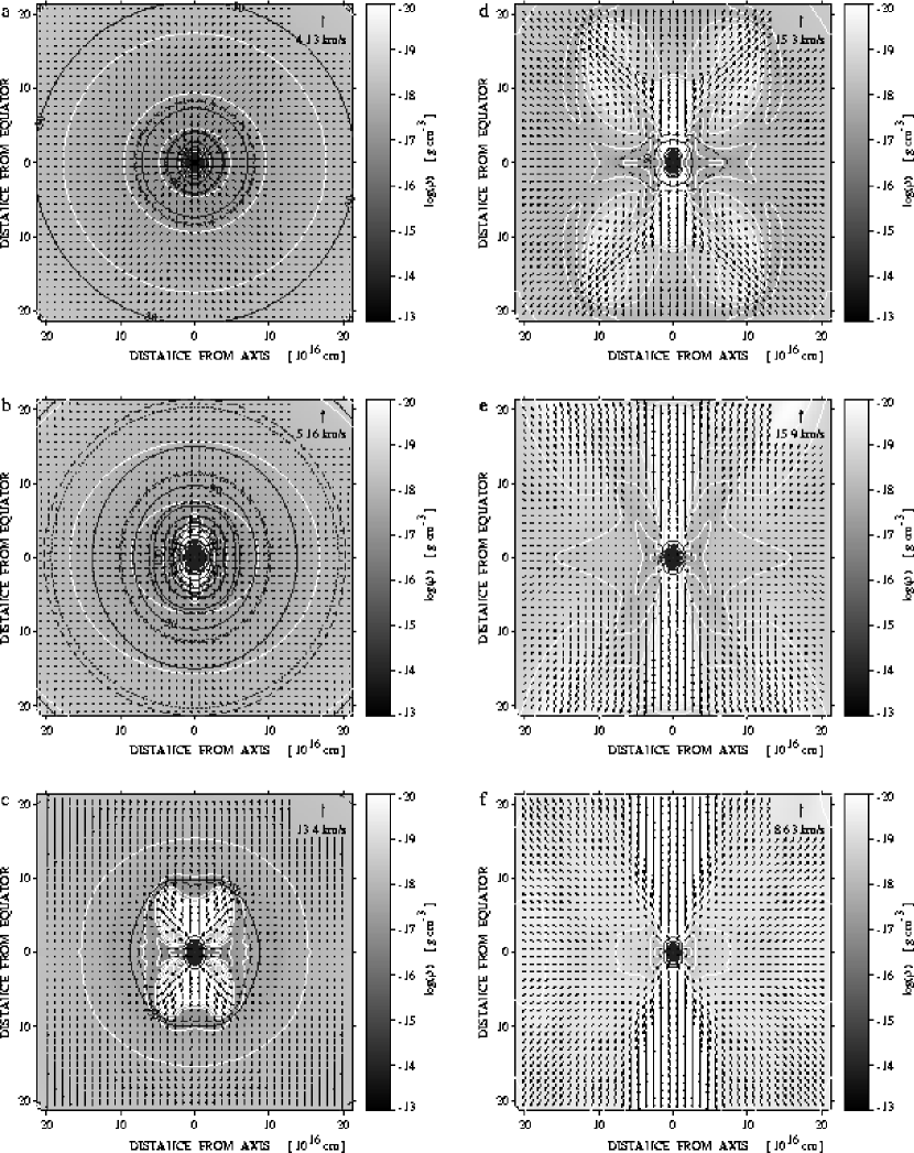
Figure 8: Distribution of density (grey-scale and white contour lines), velocity (arrows), temperature of amorphous carbon grains (solid black contour lines), and temperature of silicate grains (dotted contour lines) for case F60 (see Table 3) at evolutionary times as indicated in Table 4.

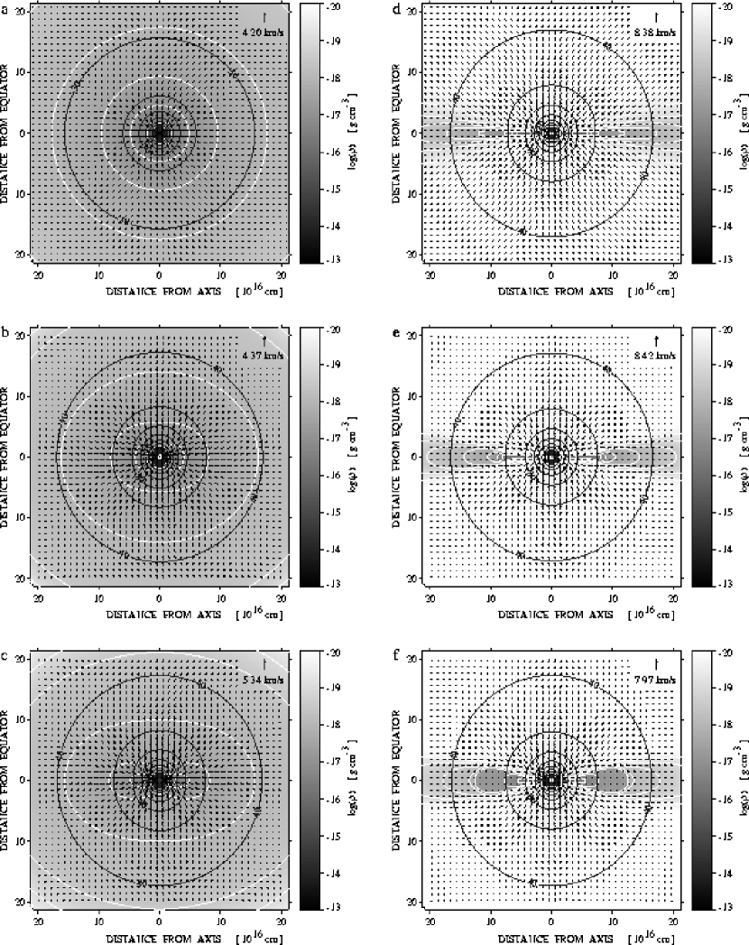
Figure 9: Distribution of density, velocity, and grain temperature for case G60 at evolutionary times as indicated in Table 4. Symbols and lines are as in Fig. 8.

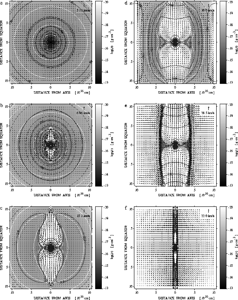
Figure 10: Distribution of density, velocity, and grain temperatures for case F30 at evolutionary times as indicated in Table 4. Symbols and lines are as in Fig. 8.

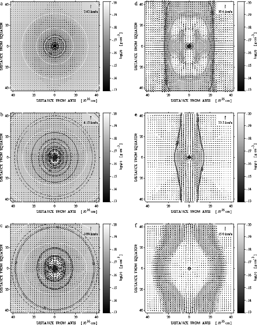
Figure 11: Distribution of density, velocity, and grain temperatures for case F120 at evolutionary times as indicated in Table 4. Symbols and lines are as in Fig. 8.

4.2.2 Case G60

Although the evolution of case G60 initially proceeds in a similar fashion as case F60, notable differences are apparent after 25 000 years (compare frame 9b to frame 8c). The flow of material into the inner zone has effectively been stopped at 15 000 years, a time at which only 20.7 M_⊙ had been accreted (see Fig. 7). Contrary to case F60 there is no indication of the formation of a polar cavity, evacuated by radiative forces, even at the most advanced evolutionary time considered, 110 000 years (frame 9f). Instead, the material flows onto a thin, disk-like structure, supported in the radial direction by both centrifugal and radiative forces.

4.2.3 Case F30

As for case F60 the initial collapse of case F30 is nearly spherically symmetric until an evacuated polar cavity is formed, encased in a system of expanding shock fronts. Here, the infalling material collides with the radiatively accelerated outflow. In the condensed cylindrical shell bounded by the shock fronts (see frame 10e) the hard radiation from the central source is absorbed and reemitted at longer wavelengths. Because of this degrading of the stellar radiation “hardness”, the material outside the cylindrical shell is able to flow radially inwards more or less parallel to the equator for $|z|<10^{17}$ cm. Material continues to flow into the central zone via the equatorial plane, and the central stellar mass ultimately grows to 31.6 M_⊙, more than originally present within the computational grid. The cylindrical shell depicted in frames 10d and 10e is a short-lived phenomenon, however. Within a few thousand years it collapses into a long, narrow, filamentary structure (frame 10f) containing about 13 M_⊙.

4.2.4 Case F120

Again, as in cases F60 and F30 discussed above, the initial collapse is spherically symmetric (frame 11a), followed by the formation of a polar cavity evacuated by radiative forces (frame 11b), after a significant amount of material has accumulated within the central zone ($M_{*}=32.9$ M_⊙ at $t=28\,000$ yr.). The central star continues to accrete an additional 10 M_⊙ via an equatorial flow through a disk-like structure over the next 30 000 years albeit at an ever decreasing rate. This “disk” is short-lived, however. At an evolutionary age of 60 000 years (frame 11d) the accretion process has stopped and a cylindrical shell first forms, contracts to a smaller cylindrical radius with a more focused polar outflow (frame 11e), and then reexpands (frame 11f). Whereas for earlier evolutionary times the gas density was higher in the equatorial regions than in the polar outflow regions, the final frame strongly resembles an expanding “cocoon” shell, punctured and elongated by a polar outflow. No disk-like structure is visible.

4.3 Appearance of Molecular Clumps

With the known density and equilibrium temperature distributions of each dust component calculated for each time step, we can perform ray-tracing radiation transfer calculations analogous to those of YB, who — by contrast — used the single dust temperature obtained in a grey radiation transfer code. From these ray-tracing calculations we can extract both SEDs (see Fig. 12 and 13) and isophote maps at selected wavelengths for any given evolutionary age.

Figure 12: SEDs at selected evolutionary ages of sequence F60. The four curves marked “a” correspond to the time shown in frame 8a, “b” to frame 8b, and “f” to frame 8f. The viewing angle $0^{\circ}$ is pole-on, $90^{\circ}$ is edge-on.

Figure 13: SEDs at selected evolutionary ages of sequence F120. The four curves marked “a” correspond to the time shown in frame 11a, “b” to frame 11b, and “f” to frame 11f.

Because, however, our spatial resolution in the innermost regions is much worse than that of YB and furthermore, we have made no attempt to model the emission from a hypothetical disk within the central cell (see YB’s “central zone disk model”), we will not be able to accurately model the emission from dust warmer than about 400 K. Even in the rather late formation stages considered here — the central stars have evolved to main sequence O-stars, very little near infrared and no optical/ultraviolet radiation escapes the remnant molecular cloud. It is reasonable to assume that a non-homogeneous distribution of material within the central zone (i.e. clumpiness or a flattened disk) would have allowed at least some of the hard photons from the central source to escape. Thus, the examples given here can only be illustrative of the basic method rather than an accurate model of the expected near infrared to ultraviolet flux. Unfortunately, our ignorance of the goings-on within the central zone preclude a more definitive treatment.

5 Discussion and Conclusions

Our improved frequency dependent radiation hydrodynamics code is able to track the infall of material within a molecular clump against radiative forces. We find that the “flashlight effect” first discussed by Yorke & Bodenheimer (1999), i.e. the non-isotropic distribution of radiative flux that occurs when a circumstellar disk forms, is strongly compounded by the frequency dependent radiation transfer. The shortest wavelength radiation (which is also the most effective for radiative acceleration) is most strongly concentrated towards the polar directions, whereas the longer wavelength radiation (less effective radiative acceleration) is more or less isotropic. We conclude that massive stars can in principle be formed via accretion through a disk, in a manner analogous to the formation of lower mass stars. A powerful radiation-driven outflow in the polar directions and a “puffed-up” (thick) disk result from the high luminosity of the central source.

We have developed a simplified model for following the evolution of accreting (proto-) stars, using existing tracks for non-accreting stars. With this model we have shown that in the case of massive star formation the energy released within the accretion shock front, the “accretion luminosity”, is not the dominant source of luminosity after a few thousand years of evolution.

The accretion rate onto the central source is time-dependent. It rises sharply after one free-fall time to a maximum value and falls off gradually (in the frequency-dependent cases). This is in contrast to the expectations of Meynet & Maeder (2000) and Behrend & Maeder (2001), who have assumed mass accretion rates $\dot{M}_{*}$ that increase monotonically in time up to a maximum value.

We have also shown that the concept of “birthline”, the equilibrium position of fully convective, deuterium-burning stars in the HR diagram with cosmic deuterium abundance, is — strictly speaking — unattainable for stars more massive than 1 M_⊙. Beginning with a protostar of a fraction of a solar mass and building up via accretion to 1 M_⊙ and higher masses, it either accretes too rapidly (shifting the HR position to smaller radii) or it accretes too slowly (significant amounts of previously accreted deuterium are consumed). For masses $M\lesssim 10$ M_⊙, however, the contribution of the accretion luminosity may make the star appear to lie on or above the birthline.

In this investigation we have not addressed the issues of the longevity of the circumstellar disk or the possible formation of a dense stellar cluster within our central computational zone rather than a single star. However, even without the assumption of ionizing radiation, we find that these disks are not long-lived phenomena. In the most massive cases the effects of radiative acceleration eventually disperse the remnant disks. Future studies will have to address the issues of ionization and the interactions of the disk with powerful stellar winds. The effects of nearby companions in a dense stellar cluster will also have to be considered in future work.

References

- Adams & Shu (1986) Adams, F.C., & Shu, F.H. 1986, ApJ, 308, 836
- Allen (1973) Allen, C.W. 1973, Astrophysical Quantities, 3rd ed., London: Athlone Press
- André et al. (2000) André, P., Ward-Thompson, D., Barsony, M. 2000, in Protostars & Planets IV, ed. V. Mannings, A.P. Boss & S.S. Russell, Tucson: Univ. of Arizona Press, p. 59
- André et al. (1996) André, P., Ward-Thompson, D., & Motte, F. 1996, A&A, 314, 625
- Auer (1987) Auer, L. 1987, in Numerical Radiative Transfer, ed. W. Kalkofen, Cambridge: Cambridge Univ. Press, p. 101
- Behrend & Maeder (2001) Behrend, R., Maeder, A. 2001, A&A, 373, 190
- Berger & Colella (1989) Berger, M.J. & Colella, P. 1989, J. Comp. Phys., 82, 64
- Bonnell et al. (1998) Bonnell, I.A., Bate, M.R., Zinnecker, H. 1998, MNRAS, 298, 93
- Bücker & Sauren (1996) Bücker, H.M. & Sauren, M. 1996, Internal Report kfa-zam-ib-9605, Research Centre Jülich
- Cabrit & Bertout (1992) Cabrit, S., & Bertout, C. 1992, A&A, 261, 274
- (11) Cannon, C.J. 1973a, J. Quant. Spectrosc. Rad. Trans., 13, 627
- (12) Cannon, C.J. 1973b, ApJ, 185, 621
- Churchwell (1998) Churchwell, E. 1998, in The Origin of Stars and Planetary Systems, eds. C. Lada & N. Kylafis, NATO Science Series, 540 (Kluwer), p. 515
- Crutcher et al. (1994) Crutcher, R., Mouschovias, T.Ch., Troland, T., & Ciolek, G. 1994, ApJ, 427, 839
- D’Antona & Mazzitelli (1994) D’Antona, F., & Mazzitelli, I. 1994, ApJS, 90, 467
- Draine & Lee (1984) Draine, B.T., Lee, H.M. 1984, ApJ, 285, 89
- Eiroa et al. (1994) iroa, C., Casali, M. M., Miranda, L. F., Ortiz, E. 1994, A&A, 290, 599
- Henning (2000) Henning, T., Schreyer, K, Launhardt, R., Burkert, A. 2000, A&A, 353, 211
- Hollenbach et al. (2000) Hollenbach, D., Yorke, H.W., Johnstone, D. 2000, in Protostars & Planets IV, ed. V. Mannings, A.P. Boss & S.S. Russell, Tucson: Univ. of Arizona Press, p. 401
- Iben (1965) Iben, I., Jr. 1965, ApJ, 141, 993
- Kippenhahn & Hofmeister (1977) Kippenhahn, R.; Meyer-Hofmeister, E. 1977, A&A, 54, 539
- Kippenhahn & Weigert (1980) Kippenhahn, R., Weigert, A. 1980, Stellar Structure and Evolution, Heidelberg: Springer Verlag
- Levermore & Pomraning (1981) Levermore, C., Pomraning, G. 1981, ApJ, 248, 321
- Lizano & Shu (1989) Lizano, S., Shu, F.H. 1989, ApJ, 342, 834 measurements Martin-Pintado et al. (1994) do find indirect
- Martin-Pintado et al. (1994) Martin-Pintado, J., Neri, R., Thum, C., Planesas, P., Bachiller, R., 1994 A&A, 286, 890
- Mathis, Rumpl, & Nordsieck (1977) Mathis, J.S., Rumpl, W., Nordsieck, K.H. 1977, ApJ, 217, 425
- Meynet & Maeder (2000) Meynet, G., Maeder, A. 2000, A&A, 361, 101
- Motte et al. (1998) Motte, F., André, P., & Neri, R. 1998, A&A, 336, 150
- Mouschovias (1990) Mouschovias T.Ch. 1990, in Physical Processes in Fragmentation and Star Formation, ed. R. Capuzzo-Dolcetta, C. Chiosi, & A. Di Fazio, Dordrecht: Kluwer, p. 117
- Preibisch et al. (1993) Preibisch, T., Ossenkopf, V., Yorke, H.W., Henning, T. 1993, A&A, 279, 577
- Press et al. (1992) Press, W.H., Teukolsky, S.A., Vetterling, W.T., Flannery, B.P. 1992, Numerical Recipes in C, 2nd ed., Cambridge: Cambridge Univ. Press
- Richling & Yorke (1998) Richling, S., Yorke, H.W. 1998, A&A, 340, 508
- Richer et al. (2000) Richer, J. S., Shepherd, D. S., Cabrit, S., Bachiller, R., Churchwell, E. 2000, in Protostars & Planets IV, ed. V. Mannings, A.P. Boss & S.S. Russell, Tucson: Univ. of Arizona Press, p. 867
- Rozyczka et al. (1994) Różyczka, M., Bodenheimer, P., & Bell, K.R. 1994, ApJ, 423, 736
- Scharmer (1981) Scharmer, G.B. 1981, ApJ, 249, 720
- Shakura & Sunyaev (1973) Shakura, N.I., Sunyaev, R.A. 1973, A&A, 24, 337
- Shepherd & Churchwell (1996) Shepherd, D. S., Churchwell, E. 1996, ApJ, 472, 225
- Shepherd et al. (2000) Shepherd, D. S., Yu, K. C., Bally, J., Testi, L. 2000, ApJ, 535, 833
- Sleijpen & Fokkema (1993) Sleijpen, G.L.G., Fokkema, D.R. 1993, Electr. Transactions on Num. Analysis, 1, 11 (etna@mcs.kent.edu)
- Sonnhalter et al. (1995) Sonnhalter, C., Preibisch, T., Yorke, H.W. 1995, A&A, 299, 545
- Stahler et al. (2000) Stahler, S.W., Palla, F., Ho, P.T.P. 2000, in Protostars & Planets IV, ed. V. Mannings, A.P. Boss & S.S. Russell, Tucson: Univ. of Arizona Press, p. 327
- Tomisaka et al. (1990) Tomisaka, K., Ikeuchi, S., & Nakamura, T. 1990, ApJ, 362, 202
- Williams et al. (2000) Williams, J.P., Blitz, L., McKee, C.F. 2000, in Protostars & Planets IV, ed. V. Mannings, A.P. Boss & S.S. Russell, Tucson: Univ. of Arizona Press, p. 97
- Yorke & Bodenheimer (1999) Yorke, H.W., Bodenheimer, P. [YB] 1999, ApJ, 525, 330
- Yorke et al. (1995) Yorke, H.W., Bodenheimer, P., Laughlin, G. 1995, ApJ, 443, 199
- Yorke & Kaisig (1995) Yorke, H.W., Kaisig, M. 1995, Comp. Phys. Comm., 89, 29
- Yorke & Henning (1994) Yorke, H.W., Henning, T. 1994, in Molecules in the Stellar Environment, IAU Coll. No. 146, ed. U.G. Jørgensen, Berlin: Springer, p. 186