Abstract

We explore various pitfalls and challenges in determining the equation-of-state ($w$) of dark energy component that dominates the universe and causes the current accelerated expansion. We demonstrated in an earlier paper the existence of a degeneracy that makes it impossible to resolve well the value of $w$ or its time-derivative with supernovae data. Here we consider standard practices, such as assuming priors that $w$ is constant or greater than $-1$, and show that they also can lead to gross errors in estimating the true equation-of-state. We further consider combining measurements of the cosmic microwave background anisotropy and the Alcock-Paczynski test with supernovae data and find that the improvement in resolving the time-derivative of $w$ is marginal, although the combination can constrain its present value perhaps to 20 percent uncertainty.

PACS number(s): 98.62.Py, 98.80.Es, 98.80.-k

1 Introduction

Measurements of Type IA supernovae have shown that the expansion of the universe is accelerating [1, 2], suggesting that most of the energy density of the universe consists of some form of dark energy with negative pressure [3]. Combining measurements of the cosmic microwave background anisotropy and observations of large-scale structure provides important corroborating evidence.[4, 5] Two candidates for the dark energy are a cosmological constant (or vacuum density) and quintessence,[6] a time-varying, spatially inhomogeneous component. In a previous paper [7] (Paper I), we addressed the question of whether supernova measurements can be used to measure the equation of state (EOS) of the negative pressure component, the ratio $w$ of the pressure to the energy density. The issue is important because $w=-1$ for a cosmological constant whereas $w$ takes on different values and can be significantly time-varying in the case of quintessence.[6, 8] Under the assumption that $w$ is constant, its value can be determined to better than 5 per cent by measuring several thousand supernovae distributed equally between red shift $z=0$ and $z=2$. However, we showed that a degeneracy opens up if $w$ is time-dependent which makes it impossible to determine accurately the current value of $w$ or its time-derivative. The cause of the degeneracy is that supernovae measure luminosity distance, which is related by a multi-integral expression to the EOS as a function of red shift, $w(z)$. Widely different $w(z)$ can have the same multi-integral value.

The purpose of this paper is to explore some pitfalls and challenges in determining the EOS and its time variation using supernovae. For example, we shall show how the standard practice of considering only models with $w\geq-1$ or only models with constant $w$ when doing likelihood analyses can lead to grossly incorrect results. For example, we will illustrate cases where the standard practice will suggest that $w$ is near -1 or much more negative than $-1$ when, in fact, $w$ is significantly greater than -1 and rapidly time varying. We shall show that a non-zero value of $dw/dz$ is more easily detected if $dw/dz>0$ than if $dw/dz<0$. We shall also contrast measuring $w$ for the negative pressure component alone ($w_{Q}$) versus the mean value for the total energy density (including ordinary and dark matter), $w_{T}$. The degeneracy problem is less severe for $w_{T}$, but this parameter provides less useful information. We consider possibilities of breaking the degeneracy between $w$ and $dw/dz$ by combining supernovae results with either cosmic microwave background anisotropy measurements and/or the Alcock-Paczynski test. We shall show that neither additional test significantly improves the measurement of the time-variation of $w$, although optimistic assumptions about the Alcock-Paczynski test suggest that the current value of $w$ can be measured to within 20 percent or so.

We conclude that a new, yet to be found test has to be devised to resolve well the cosmic EOS and its time variation. We stress that with current data it is possible to determine the EOS to about a factor of two. For a future experiment to significantly enhance the determination of the EOS, and enable the distinction between a constant EOS and a time-dependent one, it needs to resolve the equation of state at the 10% level or better.

The results of our analysis agree with many other analyses [10, 11, 12, 13, 14, 15, 16, 17, 18, 19, 20, 21], although not always with their interpretation, and can be used to explain why some other analyses seem to indicate a superior resolving power of SN measurements alone [22, 23, 24, 25], or in combination with other measurements [26, 27, 28, 29]. Some of the latter analyses implicitly assume unrealistic accuracy in independent determination of cosmological parameters, by not including self-consistently the uncertainty in $w(z)$ in all measurements. For example, assume a reported resolution of matter energy density which was based on assuming $w_{Q}=-1$.

Type IA supernovae have intrinsic variability of about 0.15 in absolute magnitude, but currently the errors in measuring distant SN are above this. There are ongoing programs to extend the search to deeper redshifts and improve measurement quality. The proposed SNAP satellite plans to measure 2000 SN per year, mostly in the range of redshifts $0.1<z<1.2$, and some as far as $z=1.7$.[30] The anticipated error in individual magnitudes is $\Delta m=0.15$ statistical and 0.02 systematic error, which yields about 1% relative error in luminosity distance $d_{L}$.

For our numerical estimates, we have generated 50 SN magnitudes randomly chosen from a uniform distribution in $z$ values, between $z=0.1$ and $z=2$. Magnitudes were generated from a Gaussian distribution with mean value $m(z)$ calculated using fiducial models. We have used our 50 points to simulate approximately 2000 SN by reducing their magnitude error by a factor $\sqrt{40}$ to 0.03 from the minimal 0.15 magnitude. Thus each generated point corresponds to 40 SNAP-like points, binned together. This corresponds to $1.4\%$ relative error in $d_{L}$. Hence, our analysis is based on a SN search more extensive than the actual SNAP proposal. To obtain a quantitative estimate of how well models are resolved, we use one of two procedures. First, we can find the maximum likelihood contours of the various models for each of the fiducial models and explore the degeneracy in parameter space. Alternatively, we can assume that all models which predict $d_{L}(z)$ within 1% of the fiducial cosmological model for all $z$ between 0 and 2 are deemed indistinguishable. We find that both approaches give comparable results. That is, the $95\%$ CL likelihood contours using the first procedure are roughly equivalent to the indistinguishability region of the second.

2 Dependence of luminosity distance on dark and total EOS

Luminosity distance is defined to be the ratio of luminosity ${\cal L}$ to flux ${\cal F}$

$$d_{L}=\sqrt{\frac{{\cal L}}{4\pi{\cal F}}}=(1+z)r,$$ (1)

where the present value of the scale factor $a_{0}$ is normalized to unity (throughout subscript 0 denotes present values); $r$ is the coordinate distance

$$r=\int_{1}^{1+z}\frac{dx}{H};$$ (2)

and $H$ is the Hubble parameter $H=\dot{a}/a$. The observed SN magnitudes are related to $d_{L}$,

$$m(z)=M+25+5\log_{10}\left[H_{0}d_{L}(z)\right],$$ (3)

$M$ being the SN absolute magnitude.

For a flat universe with two energy sources, matter (including dark matter) and a dark Q-component, there are two equivalent routes to computing $d_{L}$ without assuming any prior about the time dependence of $w_{Q}$. One way is to use the algebraic relation between the total energy density and the Hubble parameter $H$. Using conservation equations, the energy densities of the dark component $\rho_{Q}$ and that of ordinary matter $\rho_{m}$, are given by

$$\rho_{Q}(z) = (\rho_{Q})_{0}(1+z)^{3}\ exp\left[3\int_{1}^{1+z}w_{Q}\frac{dx}{x}\right]$$ (4)

$$\rho_{m}(z) = (\rho_{m})_{0}(1+z)^{3}.$$ (5)

Since

$$\left(\frac{H}{H_{0}}\right)^{2} = \frac{\rho_{m}+\rho_{Q}}{(\rho_{m})_{0}+(\rho_{Q})_{0}}$$ (6)

$$= \frac{g}{1+g}(1+z)^{3}+\frac{(1+z)^{3}}{1+g}\ exp\left[3\int_{1}^{1+z}w_{Q}\frac{dx}{x}\right]$$

where $g$ denotes the present ratio of matter to dark energy densities $g=(\frac{\Omega_{m}}{\Omega_{Q}})_{0}$, $H$ can be expressed as

$$H=H_{0}\ (1+z)^{3/2}\left(\frac{g}{1+g}+\frac{1}{1+g}exp\left[3\int_{1}^{1+z}w_{Q}\frac{dx}{x}\right]\right)^{1/2}.$$ (7)

Substituting this into $d_{L}$ gives

$$d_{L} = \frac{(1+z)}{H_{0}}(1+g)^{1/2}\int\limits_{1}^{1+z}\frac{dx}{x^{3/2}}\left[g+exp\left(3\int\limits_{1}^{x}w_{Q}(y)\frac{dy}{y}\right)\right]^{-1/2}$$ (8)

An equivalent approach is to treat the sum of dark matter and the dark energy component as a single cosmic fluid with average equation of state $w_{T}(z)=\Omega_{Q}(z)w_{Q}(z)$, where

$$w_{T}(z) = \frac{w_{Q}}{1+(\rho_{m}/\rho_{Q})}$$ (9)

$$= \frac{w_{Q}}{1+g\ exp\left[-3\int_{1}^{1+z}w_{Q}(x)\frac{dx}{x}.\right]}$$

Since $H^{2}$ is proportional to the total energy density in the universe, it can be expressed in terms of $w_{T}$ as follows

$$\left(\frac{H}{H_{0}}\right)^{2}=exp\left[3\int_{1}^{1+z}\left(1+w_{T}(x)\right)\frac{dx}{x}\right].$$ (10)

Here we have used the conservation equation for the total energy density. Using (10) we can express $d_{L}$ in terms of $w_{Q}$ as follows,

$$d_{L} = \frac{(1+z)}{H_{0}}\int_{1}^{1+z}dx\ exp\left[-\frac{3}{2}\int\limits_{1}^{x}(1+w_{T}(y))\frac{dy}{y}\right]=$$ (11)

$$= \frac{(1+z)}{H_{0}}\int_{1}^{1+z}\frac{dx}{x^{3/2}}exp\left[-\frac{3}{2}\int\limits_{1}^{x}\left(\frac{w_{Q}(y)}{1+g\ exp\left[-3\int_{1}^{y}w_{Q}(u)\frac{du}{u}\right]}\right)\frac{dy}{y}\right].$$

This expression for $d_{L}$ as a function of $w_{Q}$ has one more integral than the relation in Eq. (8), but it is pedagogically useful in demonstrating that $d_{L}$ is sensitive only to a weighted average of $w_{T}$ or $w_{Q}$ and not to their detailed time dependence.

3 Constraining dark and total EOS using SN measurements

Based on the previous sections, a number of lessons can be learned about measuring the EOS. First, the relation between $w_{T}$ and $d_{L}$ in (11) involves an integral, so we do expect some degeneracy in the determination of $w_{T}(z)$ from SN measurements. To determine the EOS of the dark energy itself, $w_{Q}$, the total energy density must be resolved into a matter component and a dark energy component. Hence, if $\Omega_{m}$ and $\Omega_{Q}$ are not known from independent measurements, determining $w_{Q}$ entails an additional uncertainty. For example, consider a flat universe with $\Omega_{T}=\Omega_{m}+\Omega_{Q}=1$. Since the matter EOS is $w_{m}=0$, it follows that $w_{T}=w_{Q}\Omega_{Q}$. Two models with different values of $w_{Q}$ may produce the same value of $w_{T}$ and, consequently, $d_{L}$, due to offsetting differences in the value of $\Omega_{m}$.

The more negative $w_{T}$ is, the faster is the expansion. Therefore, a more negative (positive) $w_{T}$ will make $d_{L}$ larger (smaller). In addition, light from earlier times (emitted at higher $z$ values) must pass through the low $z$ universe to reach us. This means that changes in $w_{T}$ at lower $z$ affect $d_{L}$ at higher $z$. The converse is not true. Changes in $w_{T}$ at high $z$ do not affect $d_{L}$ at lower $z$.

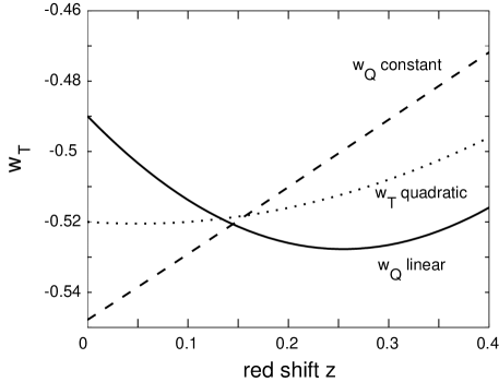
Figure 1: $w_{T}(z)$ for three best fit models of three fits under three different assumptions: constant $w_{Q}$ (dashed), linear $w_{Q}$ (solid), and quadratic $w_{T}$ (dotted), to data generated from a single fiducial model: $(w_{Q},\Omega_{m})=(-0.7-0.8z,\,.3)$. All fits prefer $w_{T}^{*}\equiv w_{T}(z^{*}\simeq.15)\simeq-.52$, but diverge for other values of $z$.

Consequently, it is not surprising that SN measurements of $d_{L}$ provide stronger constraints on $w_{T}(z)$ at low $z$ than at high $z$. In particular, if all cosmic parameters other than $w_{Q}(z)$ are fixed, there is a particular, relatively low value of $z=z^{*}$ for which $w_{T}(z)$ is most tightly constrained. This value of $z^{*}$ is clearly seen in our numerical results and was noted independently by [11, 26]. For example, Figure 1 shows the EOS $w_{T}(z)$ for three models each of which is obtained by best fit to $d_{L}(z)$ for a fiducial model $(w_{Q},\Omega_{m})=(-0.7-0.8z,\,.3)$ using one of three fitting assumptions: (1) that the dark EOS is constant; (2) that the dark EOS is linear $w_{Q}=w_{0}+w_{1}z$; and, (3) that the total EOS is quadratic $w_{T}=A+Bz+Cz^{2}$. While the real degeneracy is stronger than what is seen in the figure, we have chosen three examples to illustrate the existence of $w^{*}_{T}$ and $z^{*}$. As can be seen, the fits disagree significantly for $z$ far from $z^{*}=0.15$, but all fits agree near $z^{*}$.

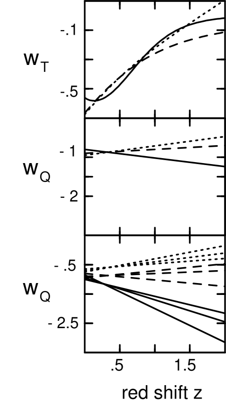
Figure 2: Models within 95% CL region of a fit to data generated from the fiducial model $(w_{Q},\Omega_{m})=(-1,0.3)$ assuming $w_{Q}=w_{0}+w_{1}z$. Top: The total EOS $w_{T}(z)$, for three different linear models. Middle: $w_{Q}(z)$ assuming $\Omega_{m}=0.3$ exactly, for the same linear models. Bottom: $w_{Q}(z)$ for nine models, assuming that $0.2<\Omega_{m}<0.4$ (no relation between the dashed, dotted and solid lines of the bottom panel to those of the middle and top ones).

Unfortunately, the resolution of $w_{Q}(z^{*})$, the quantity which most interests us, is degraded when we do not fix $\Omega_{m}$ but, instead, allow for the current uncertainty in its value. In Fig. 2, we show some linear fits to simulated data generated from the fiducial model $(w_{Q},\Omega_{m})=(-1,.3)$. The fits are representative examples which fit the fiducial model to within the 95% confidence region. The upper plot shows that $w_{T}(z)$ (with $\Omega_{m}$ fixed at 0.3) is relatively well resolved, and particularly well resolved at around redshift $z^{*}=.3$. The resolution is not that sharp in the middle plot which shows the corresponding $w_{Q}$, but a special point of enhanced resolution around $z=.4$ is still clearly seen. If one lets $\Omega_{m}$ vary in the realistic range of $0.2-0.4$, then $w_{Q}$ becomes poorly resolved and the spread at $z^{*}$ increases significantly. Similarly the spread in $w^{*}$ and $z^{*}$ increases significantly if more general functional forms of the EOS are considered.

We would like to stress that the constant or linear forms of $w_{Q}$ that we use are not meant to be anything more than simple concrete examples to highlight the fact that we are dealing with a degenerate parameter space. Showing that if one assumes a linear $w_{Q}(z)$, then it can be resolved to, say, 50% does not logically mean that it can be measured to 50% accuracy generally since $w_{Q}(z)$ is resolved with different accuracy depending on its functional form. This can be illustrated with the following examples. In Fig. 3, the difference in magnitude ($\Delta m$) for models with various EOS is shown. There are three clusters of points, each of which corresponds to a simulation of SN data for pair of different models. Each pair consists of a constant and linear $w_{Q}$. Each pair can be clearly separated from other pairs but the constant and linear “members” of a pair cannot be distinguished by SN data. The examples chosen for Fig. 3 have unrealistic large derivatives (of order unity) and therefore start to diverge from their constant partners for large $z$. More realistic examples with smaller derivatives or oscillatory behaviour will be much harder to distinguish from a constant EOS.

Clearly the treatment of the SN analysis is important. If it is assumed that $w_{Q}$ is constant, the figure shows that different values can be resolved to high accuracy, but if the assumption of constancy is relaxed and a linear $z$ dependence is allowed it becomes clear that the data can determine well only a single relation between $w_{0}$ and $w_{1}$ and that $w_{Q}(z)$ is poorly resolved.

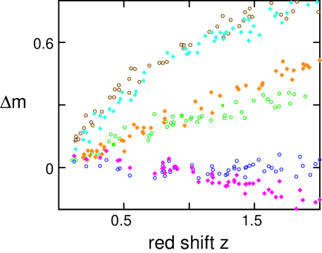
Figure 3: Magnitude differences between pairs of degenerate models and a flat pure matter ($\Omega_{m}=1$) Universe. Each pair consists of simulated data points generated from one constant $w_{Q}$ model (open circles) and one linear $w_{Q}$ model with a large (positive or negative) derivative (full squares). The pairs are well separated but it is hard to separate between “members” of each pair.

The degree of degeneracy exhibited in the $w_{Q}=const.$ fits depends on whether $w_{Q}$ is positive or negative. Recall that if different models yield a total EOS $w_{T}=w_{Q}\Omega_{Q}$ that is approximately equal, they are degenerate, and therefore changes in $w_{Q}$ can be compensated by changes in $\Omega_{Q}$ (or equivalently, in $\Omega_{m}$). The difference between the case where $w_{Q}$ is positive is due to the specific way in which this compensation mechanism operates. If $w_{Q}$ is positive, the curvature of degeneracy lines in $(w_{Q},\Omega_{m})$ plane is positive, as shown in the right panel of Fig. 4 for a fiducial model with $w_{Q}=+0.5$. Conversely, if $w_{Q}$ is negative, the curvature of the degeneracy line in $(w_{Q},\Omega_{m})$ plane is negative, as demonstrated in the left panel of figure 4. We have found that this result is unaffected by the value of the derivative of $w_{Q}$, even if it is quiet large.

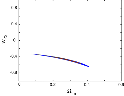
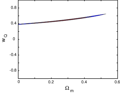
Figure 4: 95% CL contours of fits to data generated from two fiducial models. The curvature of degeneracy contours is positive for a positive $w_{Q}$ fiducial model (right) and negative for a negative $w_{Q}$ fiducial model (left).

4 Common Practices and Pitfalls in Determining $\bf w_{Q}(z)$

The previous section (and Paper I) show that the determination of $w_{Q}(z)$ from SN data is a more delicate process than it would seem. If we know a priori that $w_{Q}$ is constant, then its value can be determined quite accurately. However, without this assumption, $w_{Q}$ is poorly determined, and matters much get much worse if $\Omega_{m}$ is uncertain.

The analysis can be further confounded if certain common practices are followed. For example, many analyses assume that $w_{Q}$ is constant and presume that, even if $w_{Q}$ is time-varying, the constant- $w_{Q}$ fit will provide the mean value over recent epochs. Another common practice is to impose the condition that $w_{Q}(z)$ be limited to $-1\leq w_{Q}(z)\leq 1$, based on the positivity and stability conditions that apply to most (but not all) forms of dark energy. We shall see that both practices can produce enormous distortions of the likelihood surface that lead to grossly incorrect conclusions.

For example, we have tried to fit data generated from a fiducial model with $w_{Q}=-.7+.8z$, and $\Omega_{m}=.3$ over a redshift range $0<z<2$. Note that the fiducial model has $w_{Q}>-1$ for all $z$. Yet, if we do a best-fit assuming the prior that $w_{Q}$ is constant, we find it to be $(w_{Q},\Omega_{m})\simeq(-1.75,.65)$. Not only does the best-fit have $w_{Q}<-1$, but the whole 95% confidence contour lies in a region where $w_{Q}<-1$. The results are the elongated contours in the lower part of Fig. 5. The reason for such a strange result can be understood from the functional dependence of $d_{L}$ and $w_{Q}$. Assuming that $w_{Q}(z)=w_{0}+w_{1}z$, the energy density of the dark component is given in eq.(4),

$$\rho_{Q}=(\rho_{Q})_{0}(1+z)^{3(w_{0}-w_{1}+1)}\,{\rm exp}[3w_{1}z],$$ (12)

so increasing $w_{1}$ and decreasing $w_{0}$ have opposite and compensating effects, which tend to cancel each other’s influence on $d_{L}$. The exponential factor determines the quantitative details of this compensation since changes in $w_{0}$ need to compensate also for changes in the exponential factor. It is therefore clear that the compensation cannot be perfect over a range of $z$’s. If we insist on the prior of constant EOS (i.e., $w_{1}=0$), the fitting procedure will pick out a value of $w_{0}$ which is much more negative than the fiducial value. In the figure we have picked a fiducial with a large positive derivative to illustrate our point, but it is clear from our discussion that the same problem arises when time dependence is weaker, or in cases that the EOS has a more general functional form.

Introducing a prior that $w_{Q}>-1$ can give a very misleading impression of how well $w_{0}$ is resolved. For example, suppose that we assume the priors that $w_{Q}$ is constant and $w_{Q}>-1$, as is standard practice. The results are shown in Fig. 5, the small contours truncated at $w_{Q}=-1$. They seem to suggest that the data supports the conclusion that $w_{Q}=-1$ with a high level of confidence. The best fit is $(w_{Q},\Omega_{m})\simeq(-1,.58)$. Yet, this is not related in any obvious way to the fiducial model, $w_{Q}=-0.7+0.8z$ and $\Omega_{m}=0.3$. The values of $\chi^{2}$ per degree of freedom for the best fit models of Fig. 5 are reasonable, .95 for the unconstrained fit, and 1.39 for the constrained fit. So, what appears to be a compelling result is actually a total distortion. Of course, it is also conceivable that the actual $w_{Q}(z)$ is less than $-1$, in which case the same procedure of introducing a prior would falsely suggest that $w=-1$ fits well.

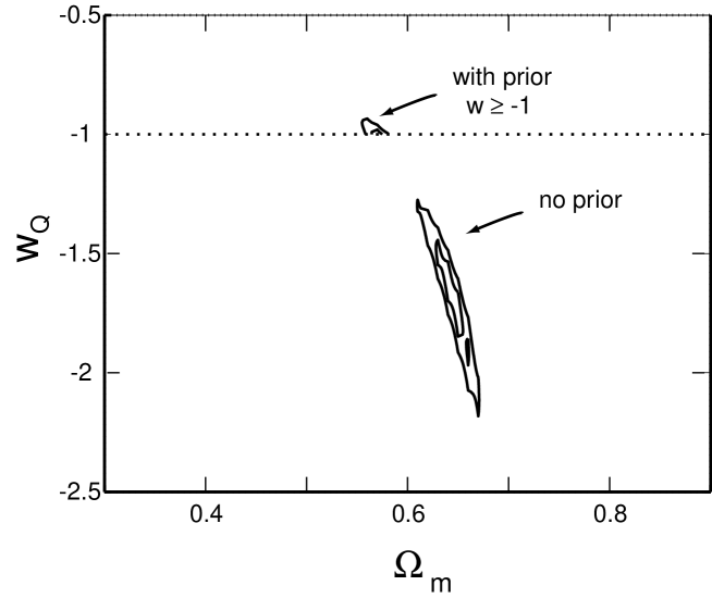
Figure 5: Constrained (small) and unconstrained (larger and more negative) 68% and 95% confidence contours of a fit to data generated from a fiducial model with linear $w_{Q}$ $(w_{Q},\Omega_{m})=(-.7+.8z,.3)$. The fit is done under the (wrong) assumption that $w_{Q}$ is constant.

5 Asymmetry in determination of the time dependence of the dark EOS

An EOS in which $w(z)$ has a large positive time derivative is easier to detect than one which has a large negative time derivative. In either case, the derivative must be large to be detected, as pointed out in Paper I, but here we are demonstrating that the challenge is asymmetric. The point is illustrated in Fig. 6. The middle panel shows a fiducial model with a modest value of $w_{1}=0.2$, and, as can be seen, this case cannot be distinguished from a model in which $w_{1}=0$. That is, the 95% CL contours overlap the line $w_{1}=0$, corresponding to no time variation. The left and right panels show cases in which $w_{1}=0.8$ and $-0.8$, respectively. The contours for the $w_{1}=0.8$ case (left) lie far from the $w_{1}=0$ line, so the time variation is detectable in this example. On the other hand, the contours for the $w_{1}=-0.8$ case (right) overlay the $w_{1}=0$, so the time-variation is not resolved.

   

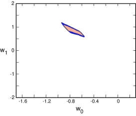
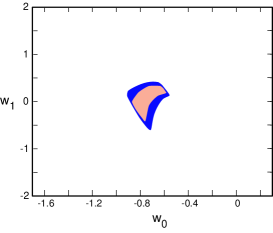
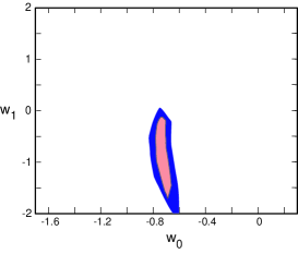
Figure 6: Likelihood contours (68% (lighter) and 95% (darker) C.L.) in the $(w_{0},w_{1})$ plane, for fits to data generated from 3 different fiducial models. LEFT: $(w_{0},w_{1},\Omega_{m})=(-0.7,0.8,0.3)$. MIDDLE: $(w_{0},w_{1},\Omega_{m})=(-0.7,0.2,0.3)$. RIGHT: $(w_{0},w_{1},\Omega_{m})=(-0.7,-0.8,0.3)$. Only the results shown in the left panel are inconsistent with a constant ($w_{1}=0$) $w_{Q}$ model.

This effect can be explained by considering the variation of the total average EOS $w_{T}$ with respect to $w_{1}$, $\Delta w_{T}=f(w_{1})\Delta w_{1}$:

$$f(w_{1})=\Omega_{Q}\left[z+3w_{Q}\left(z-ln(1+z)\right)(1-\Omega_{Q})\right].$$ (13)

We consider $w_{T}$ because the measurements of $d_{L}$ are directly sensitive to $w_{T}$, so that models can only be distinguished if they have different $w_{T}$. As can be seen from eq.(13), $w_{T}$ is much less sensitive to changes in $w_{1}$ when it is negative than when it is positive, mainly due to the value of $\Omega_{Q}$ being larger for positive values of $w_{1}$, We conclude that, in order to detect that $w_{Q}$ is time-dependent, it must be that the time-variation is large, roughly $w_{1}>0.5$, and it helps if $w_{1}$ is positive. This corresponds to the case where acceleration is becoming stronger as time evolves.

6 Combining Supernovae with other Approaches

Measurements to determine the EOS of the dark energy can be direct or indirect. Direct methods, such as SNIa observations, the Alcock-Paczynski (AP) test [31], and the cosmic microwave background (CMB) attempt to measure the Hubble parameter $H$, its derivative $H^{\prime}$ and $\Omega_{m}$, or some function of them. Indirect methods, such as structure formation aspects of the CMB and measurements of large scale structure (LSS) try to infer $w_{Q}(z)$ from its effects on structure evolution.

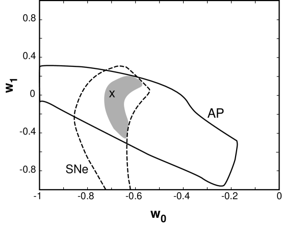
Figure 7: Two-sigma contours in the $(w_{0},w_{1})\equiv(w_{Q}(z=0),\,dw_{Q}/dz_{0})$ plane for two idealized experiments. One measures thousands of supernovae between $z=0$ and $z=2$ (dashed contours). The supernovae are divided into 50 bins with a net error of 1.4% per bin. The second experiment is an optimistic estimate for the AP test (solid contours), assuming 50 bins of Lyman-alpha clouds uniformly distributed between $z=1.5$ and $z=3$ with each bin measured with an accuracy of 3%. Both experiments assume a fiducial model with $\Omega_{m}=0.3$, $\Omega_{Q}=0.7$, $w_{Q}=-0.7=const.$, indicated by the X. In both experiments $\Omega_{m}$ is marginalized over the range 0.2 to 0.4. The two-sigma joint likelihood for the two observations is shown in the shaded region.

An example of a complementary observation is the the Alcock-Pazcynski (AP) test. The physical transverse size of an object is given by $d_{T}=d_{A}\Delta\theta=\frac{r}{1+z}\Delta\theta$, $d_{A}$ being the angular distance and $\Delta\theta$ the observed angular size. The physical radial size is $d_{R}=\int\sqrt{g_{rr}}dr=\frac{1}{(1+z)H(z)}\Delta z$. For a population of spherical objects, the AP test is given by equating the transverse and radial sizes: $AP(z)=\frac{\Delta z}{\Delta\theta}=H(z)r(z)=H(z)\int_{1}^{1+z}\frac{dx}{H}.$

The AP test on its own is not expected to improve the resolution of the dark EOS since it has a more complex dependence on $w_{Q}$ than $d_{L}$. What does seem promising, as pointed out by McDonald [32, 33], is that the AP test can further constrain the range of $\Omega_{m}$.

Fig. 7 shows the likelihood contours assuming optimistic anticipated errors over a continuous range between $z=0$ and $z=2$ of 1.4% for $d_{L}$, and, for the AP test, 50 bins between redshift $z=1.5$ and $z=3$ measured with 3% error per bin.[33] Both simulations represent highly optimistic assumptions about future measurements. The results are interesting. The better constraint on $\Omega_{m}$ from the AP test reduces the uncertainty in $w_{0}$, but does not significantly change the uncertainty in the time-variation, $w_{1}$. This is not surprising since even a perfect determination of $\Omega_{m}$ would leave a considerable uncertainty in $w_{1}$, as shown in Paper I. To be sure, the Alcock-Paczynski test is useful and worth pursuing, and a highly precise measurement combined with a highly precise measurement of SNe could determine the present value of $w$ to within 15 or 20 percent. However, it does not help significantly with the particular problem of pinning down the time-variation of the equation-of-state.

Measurements of the CMB anisotropy provide an additional probe of $w(z)$. This probe also suffers from a degeneracy problem, even in the case where $w$ is constant. The positions of the acoustic peaks in the temperature anisotropy power spectrum depend on the angular distance ($d_{A}$) to the last scattering surface which, just like the luminosity distance for supernovae, depends on a multi-integral over $w(z)$, $d_{A}=d_{L}/(1+z)^{2}$. In addition, the heights of the peaks depend on $\Omega_{Q}$ and the Hubble parameter, $H_{0}=h\ 100\ {\rm km/parsec/sec}$. When all effects are considered, then, as shown by Huey, et al. [34], the power spectrum is unchanged as certain combinations of $\Omega_{m}$, $h$, and $w$ are varied. Consequently, none of these parameters can be determined well by the CMB data alone. Instead, measurements can only constrain these parameters to a thin two-dimensional surface in this three-dimensional parameter subspace.

The reason why one might be optimistic about combining CMB anisotropy and SN measurements is that the degeneracy surface for the CMB anisotropy measurements is nearly orthogonal to the degeneracy surface for the SN measurements for the case of constant $w$. Figure 8 illustrates the small overlap between the SN and CMB degeneracy regions in the $\Omega_{m}$-$w$ plane. Other authors have considered adding the CMB contribution[26, 27] but they have not included the degeneracy aspect. As we shall show below, introducing time-varying $w(z)$ introduces additional degeneracy that spoils the resolution even when the SN and CMB anisotropy measurements are combined.

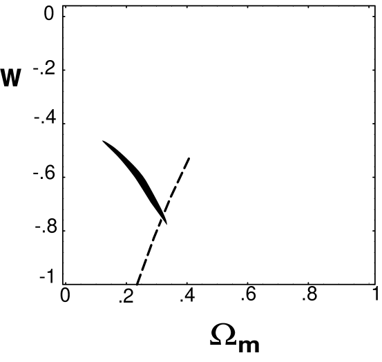
Figure 8: A simulation of the problem that arises if one assumes $w(z)$ is constant in the fitting procedure. For a given fiducial model, the likelihood fit for the CMB anisotropy (dashed line) and SN luminosity distance-red shift (contour) observations are illustrated. The degeneracy curve for the CMB assumes cosmic variance limited sampling, and the SN contour assumes 1% error in luminosity distance. Each degeneracy region is long and thin, and the two are nearly orthogonal. Based on the small overlap, one is tempted to conclude that constancy of $w$ is well established and its value is well determined. However, that conclusion is absolutely wrong. The fiducial model in this example actually has a rapidly time-varying $w(z)=-2/3-1/6z$ for $z<2$ and $w(z)=-1$ for $z>2$. The degeneracy regions were computed assuming $w_{1}=0$, but, if $w_{1}$ is fixed at a value somewhat less than zero, say, there are once again two narrow degeneracy regions which intersect over a small region, but the value of $w_{0}$ in the overlap region is significantly shifted. That is, the two experiments produce two degeneracy surfaces that intersect along a curve in the $w_{1}$ direction along which a degeneracy remains.

Rather than do another complete survey, which is a major technical challenge on its own, we illustrate the degeneracy in parameter space with a simple example in which we consider the family of $w(z)$ of the form:

$$w(z) = w_{0}+w_{1}\,z\;\;\;{\rm for}\;z<2$$ (14)

$$= w_{0}+2\,w_{1}\;\;\;{\rm for}\;z\geq 2$$

This form was chosen to allow significant time variation recently when $\Omega_{Q}$ is large and, in particular, to be similar to the models considered in Paper I for $z<2$. For $z<2$, the degeneracy problem with respect to SN data was already demonstrated and the $w_{0}$-$w_{1}$ degeneracy region was characterized. However, we could not simply maintain the linear change in $w(z)$ with respect to $z$ out to the last scattering surface at $z=1000$ because the value of $w$ would be ridiculously non-physical. Hence, we cutoff the $z$-dependence at a value of $z$ where $\Omega_{Q}$ is negligible and $w(z)$ is physically plausible. We, then, maintain that condition back to the last scattering surface. For example, for $w=-2/3-1/6z$ and $(\Omega_{Q})_{0}=.7$, at $z=2$ the dark energy contribution to the total energy density is less than 15%, which makes the details of the $z$-dependence cutoff unimportant. From $z=2$ until last scattering surface, this model will have $w=-1$.

The value of $w_{0}$ in our time-varying examples is fixed to be $-2/3$ except where otherwise stated. In each of these models, we also have $h=.65$, $\Omega_{Q}=.7$, $\Omega_{m}=.3$, and $\Omega_{b}=.04$. Here $\Omega_{b}$ is the baryon density and $\Omega_{m}$ is the total matter density (baryonic plus non-baryonic). Note that luminosity distance-red shift measurements are not sensitive to $\Omega_{b}/\Omega_{m}$, but the CMB measurements are.

The time-varying models were treated as the fiducial model, and then a numerical search was performed for a constant EOS model that is indistinguishable from the fiducial model based on the combined measurement of the CMB and of supernovae. Models were considered degenerate under the combined tests if: (1) the percent difference between the luminosity distance-redshift predictions for the two models is less than one percent out to $z=2$ (the same criterion as in Paper I); and, (2) the CMB predictions for the two models assuming a full-sky cosmic-variance limited measurement (no experimental error) cannot be distinguished to better than 3$\sigma$. Both criteria are based on optimistic predictions of what will be realistically possible.

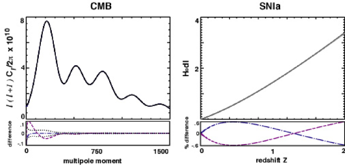
Figure 9: Illustration of the degeneracy problem for a model with constant $w$ and two models with time-varying $w$ as discussed in the text. The upper left hand panel compares the CMB power spectra. The lower left shows the differences between the time-varying models and the constant $w$ model and shows that they are less than or comparable to the full-sky cosmic variance theoretical uncertainty, the envelope shown in the figure (dotted lines). The upper right panel compares predictions for the luminosity distance-red shift relation. The lower right panel shows the differences with respect to constant model are less than the 1% resolution anticipated from supernovae measurements.

For the CMB, distinguishability between a model with a constant $w$ and a fiducial with a time-dependent $w$ was determined by a log-likelihood analysis. The log-likelihood was calculated according to the log-likelihood formula obtained by Huey, et al.[34];

$${\cal L}_{FC}=-\sum_{l}(\ell+\frac{1}{2})\times\left(1-\frac{C_{\ell}^{(F)}}{C_{\ell}^{(C)}}+\log\frac{C_{\ell}^{(F)}}{C_{\ell}^{(C)}}\right).$$ (15)

The coefficients $C_{\ell}^{(F)}$ and $C_{\ell}^{(C)}$ are the CMB multiple moments corresponding to the fiducial and constant equation of state models, respectively.

Fig. 8 illustrates the problem that arises if one assumes $w(z)$ is constant in the fitting procedure. We have already observed that this distorts results for the case of SN data alone. Here we show that the problem remains if CMB data is co-added. Assuming $w$ is constant ($w_{1}=0$), both measurements produce a thin degeneracy region in the $\Omega_{m}$-$w$ plane. Based on the small overlap, one is tempted to conclude that constancy of $w$ is well established and its value is well determined. However, this conclusion is absolutely wrong. In this example, the fiducial model actually has a rapidly time-varying EOS $w(z)=-2/3-1/6z$ for $z<2$ (which produces a change in $w$ of 50% over this range), and $w(z)=-1$ for $z>2$. The degeneracy regions were computed assuming $w_{1}=0$. If $w_{1}$ were to be fixed at a different value, once again the two measurements will give two narrow degeneracy regions with a small overlap, but the value of $w_{0}$ in this overlap region is significantly shifted. For example, as shown in Fig 8, fixing $w_{1}=0$ results in $w_{0}=-.74$ with a few percent error. However, if $w_{1}$ were to be fixed at its correct value $w_{1}=-1/6$, the result would have been $w_{0}=-2/3$, again with a few percent error. But the central values differ by more than 10%. It is clear, then, that the two measurements produce two degeneracy surfaces which intersect along a degenerate curve which passes through a range of models with varying values for $w_{0}$ and $w_{1}$, that remain degenerate under the combined observations. For more complicated functional forms of $w_{Q}(z)$ the degeneracy curve becomes a more complicated higher dimensional surface, and the range of degeneracy in parameter space (say, for $w_{0}$) increases.

The complications in the process of extracting the EOS from both measurements are further illustrated in Fig. 9. There we show two time-varying models with slopes $|w_{1}|>0.1$, one of which is degenerate (by the log-likelihood test) with a constant $w$ model with $w=w_{0}=-.72$ and $\Omega_{b}=.04$, $\Omega_{m}=.27$, $\Omega_{Q}=.69$, and $h=.64$. The other can be barely resolved making the most optimistic estimates about cosmic variance. A slight decrease in $w_{1}$, or a slight decrease in experimental sensitivity would render the second model degenerate. The lower two plots magnify the differences between the predictions of the models. For the case of the CMB, we have also shown the envelope based on the constant $w$ model corresponding to the full-sky cosmic variance limit. For the SN, we have constrained the limits to lie between $\pm 1$%.

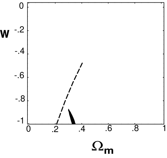
Figure 10: The same as Fig. 8 but with a fiducial model with $w_{1}=1/3$. For cases like this with very rapid time-variation in $w$, a symptom is that the CMB and SN degeneracy regions do not overlap. For $w_{1}$ large and positive, as in this example the SN contour (solid black) lies to the right of the very thin CMB degeneracy region (dashed curve). For $w_{1}$ large and negative, the SN contour lies to the left.

If $|w_{1}|$ is larger than 1/6 for our particular form of $w(z)$, we find that there is no overlap between the degeneracy curve picked out by CMB measurements and the degeneracy contour picked out by SN measurements (where both fits assuming $w$ is constant). An example is shown in Fig. 10. In the case of negative (positive) $w_{1}$ the CMB measurements that fit best suggest low (high) $\Omega_{m}$ whereas the SN measurements suggest high (low) $\Omega_{m}$. If this absence of overlap were to be found in the real data, an interpretation to pursue is that $w$ is rapidly time-varying. Yet such an extreme scenario is not favoured by most theoretical models, most of which predict a moderately time-varying $w$. For the more likely case, in which the two measurements do overlap, combining them reduces degeneracy by only a modest amount, generally not even enough to decide whether the dark energy in the universe has a time varying equation of state or not.

Co-adding the CMB to the SN data represents an improvement in the sense that $w_{1}$ and $w_{0}$ are more constrained than with SN data alone based on our earlier analysis or in Paper I. The improvement is by a factor of four or so assuming a linear form for $w(z)$, which is significant. However, there remains a large uncertainty in the EOS. Furthermore, we would stress once again that the accuracy in determining $w$ strongly depends on its assumed functional form. The range of degeneracy obtained for $w_{1}$ (a bit more than $\pm 0.1$) in our example underestimates the degeneracy for general $w(z)$. For example, for parabolic forms, the uncertainty in $w_{1}$ blows up to $\pm 0.5$. Given the extraordinarily precise data that has been brought to bear, the allowed variation in $w_{0}$, $w_{1}$ and $\Omega_{m}$ is disappointing.

7 Conclusions

An important challenge for observational cosmology is to measure the equation of state of the dark energy, $w_{Q}(z)$. This can provide important information about the fundamental physics that is responsible for the accelerated expansion of the universe. Measurements of the distance-red shift relation using supernovae, perhaps combined with other direct methods such as the Alcock-Paczyinski test or the cosmic microwave background, would appear to be promising methods. Indeed, analyses based on the a priori assumption that $w_{Q}(z)$ is constant suggest that $w_{Q}$ can be resolved to 5% accuracy or better.

In this paper and Paper I, though, we have uncovered a number of problems and pitfalls that arise when trying to determine $w_{Q}(z)$ without making prior assumptions. Our lessons may be summarized as follows:

• Because measures of luminosity or angular distance depend on integrals over $w_{Q}(z)$, a first degeneracy problem arises in which neither the current value and nor its time-variation can be resolved to any useful accuracy. (Sec. II)

• Since the effect of dark energy on the luminosity distance depends on the combination $w_{Q}\Omega_{Q}$ rather than $w_{Q}$ itself, a second degeneracy problem arises in which $w_{Q}$ and $\Omega_{Q}$ are changed simultaneously so as to keep $w_{Q}\Omega_{Q}$ fixed. (Sec. III)

• Although SN measurements may extend to $z=2$, they are most sensitive to the behavior of $w_{Q}(z)$ at a modest value of $z^{*}\approx 0.1-0.4$. (Sec. III)

• Consequently, if there were only the first degeneracy problem, $w_{Q}(z)$ could be well-resolved at $z=z^{*}$ even though it is not well-resolved for other values of $z$. Unfortunately, the resolution of $w_{Q}(z^{*})$ is totally degraded when one includes uncertainty in $\Omega_{Q}$ and the second degeneracy problem. (Sec. III, especially Fig. 2)

• The common practice of fitting data assuming that $w_{Q}(z)$ is constant can lead to grossly distorted results. Similarly, the common practice of assuming $w_{Q}\geq-1$ can lead to grossly distorted results. Fig. 5 shows a dramatic example in which these practices lead to the conclusion that $w_{Q}=-1$ and is well-resolved when, in reality, $w_{Q}>-1$ and rapidly increasing. (Sec. IV)

• Time-variation of $w_{Q}$ is more easily detected if $w_{Q}(z)$ is an increasing function of $z$ rather than decreasing. (Sec. V)

• To resolve $w_{Q}(z)$ with supernova data, an additional test is needed. Given optimistic estimates of experimental uncertainties, the Alcock-Paczynski test combined with the supernovae measurements can constraint the current value of $w$ to within 20 percent or so. However, Neither the Alcock-Paczynski test nor microwave background anisotropy measurements provide the needed resolution to constrain the time-variation. (Sec. VI)

Our principal conclusion is that a new test is required to achieve the goal of measuring $w_{Q}(z)$. In devising a new test, the two considerations must be precision and model dependence. Thus far, among the measurements that we have considered, the measurements which are precise give constraints on $w_{Q}$ that are highly model dependent, leading to degeneracy problems. Tests which are not model dependent turn out to be difficult to measure precisely. So, there lies the challenge.

In considering alternatives, it is critical to include practical estimates of their uncertainties. Furthermore, one must consider how the new tests, themselves, depend on $w_{Q}(z)$. For example, claims have been made that $\Omega_{m}$ and $\Omega_{Q}$ have been or will be measured very accurately by measurements of the cosmic microwave background [35]. However, those estimates are based on assuming that $w_{Q}=-1$. Making no prior assumption about $w_{Q}(z)$, a degeneracy problem once again arises[34] that spoils the resolution of $\Omega_{Q}$ and $w_{Q}(z)$, as discussed in Sec. VI.

While trying to devise a new test to determine $w_{Q}$, it is worth mentioning that a precise measurement of $H^{\prime}$ will be extremely useful. The dependence of $w_{Q}$ on $H$, $H^{\prime}$ (prime denotes a derivative with respect to $x=1+z$) and $\Omega_{m}$ is given by $w_{Q}=\frac{\frac{2}{3}xHH^{\prime}-H^{2}}{H^{2}-\Omega_{m}H_{0}^{2}\ x^{3}}.$ A good measurement of $H^{\prime}$ is clearly crucial to the resolution of $w_{Q}$, but current tests do not probe $H^{\prime}$ directly. The next best option is to measure $H(z)$, and then estimate $H^{\prime}$ by calculating its derivative. Obviously, this worsens the resolution for $H^{\prime}$ and increases the uncertainty in $w_{Q}$.

Three additional approaches that we have not tried yet are measuring the time dependence of structure growth on $w(z)$;[36] gravitational lensing; and direct measurements of $dz/dt$ (to be discussed elsewhere[37]).

8 Acknowledgments

We thank A. Albrecht, G. Efstathiou, D. Eichler, P. McDonald, and B. Paczynski for helpful comments, and D. Oaknin for valuable programming assistance. This research was supported by grant No. 1999071 from the United States-Israel Binational Science Foundation (BSF) (IM and RB) and by the US Department of Energy grant DE-FG02-91ER40671 (JM and PJS).

References

- [1] S. Perlmutter, et al., Ap. J. 517, 565 (1999).
- [2] A.G. Riess, et al., Ap. J. 116, 1009 (1998).
- [3] S. Perlmutter, M. S. Turner and M. White, Phys. Rev. Lett. 83, 670 (1999); P. Garnavich, et al., Ap. J. 509 74 (1998).
- [4] See, for example, J. P. Ostriker and P.J. Steinhardt, Nature 377, 600 (1995); L.M. Krauss and M.S. Turner, Gen. Rel. Grav.27, 1137 (1995).
- [5] See, for example, N. Bahcall, J.P. Ostriker. S. Perlmutter, and P.J. Steinhardt, Science 284, 1481-1488, (1999) and references therein.
- [6] R.R. Caldwell, R. Dave and P.J. Steinhardt, Phys. Rev. Lett. 80, 1582 (1998).
- [7] I. Maor, R. Brustein and P. J. Steinhardt, Phys. Rev. Lett. 86, 6 (2001).
- [8] N. Weiss, Phys. Lett. B 197, 42 (1987); B. Ratra and J.P.E. Peebles, Ap. J. , 325, L17 (1988); C.Wetterich, Nucl. Phys. B302, 668 (1988), and Astron. Astrophys. 301, 32 (1995); J.A. Frieman, et al. Phys. Rev. Lett. 75, 2 077 (1995); K. Coble, S. Dodelson, and J. Frieman, Phys. Rev. D 55, 1851 (1995); P.G. Ferreira and M. Joyce, Phys. Rev. Lett. 79, 4740 (1997); Phys. Rev. D 58, 023503 (1998); C. Armendariz-Picon, V. Mukhanov, and P.J. Steinhardt, Phys. Rev. Lett. 85, 4438-41 (2000).
- [9] G. Efstathiou, MNRAS 310, 842 (1999).
- [10] S. Podariu, P. Nugent and B. Ratra, Astrophys. J. 553, 39 (2001).
- [11] P. Astier, astro-ph/0008306.
- [12] J. Weller and A. Albrecht, Phys. Rev. Lett. 86, 1939 (2001).
- [13] T. Chiba and T. Nakamura, Phys. Rev. D 62, 121301 (2000).
- [14] V. Barger and D. Marfatia, Phys. Lett. B 498, 67 (2001).
- [15] M. Chevallier and D. Polarski, Int. J. Mod. Phys. D 10, 213 (2001).
- [16] M. Goliath, R. Amanullah, P. Astier, A. Goobar and R. Pain, astro-ph/0104009.
- [17] N. Trentham, astro-ph/0105404.
- [18] E. H. Gudmundsson and G. Bjornsson, astro-ph/0105547.
- [19] J. Weller and A. Albrecht, astro-ph/0106079.
- [20] S. C. Ng and D. L. Wiltshire, Phys. Rev. D 64, 123519 (2001).
- [21] Jens Kujat, Angela M. Linn, Robert J. Scherrer, David H. Weinberg, astro-ph/0112221.
- [22] D. Huterer and M.S. Turner, Phys. Rev. D 60, 081301 (1999).
- [23] T. D. Saini, S. Raychaudhury, V. Sahni and A. A. Starobinsky, Phys. Rev. Lett. 85 (2000) 1162.
- [24] B. Boisseau, G. Esposito-Farese, D. Polarski and A. A. Starobinsky, Phys. Rev. Lett. 85, 2236 (2000).
- [25] Y. Wang and P. M. Garnavich, Astrophys. J. 552, 445 (2001).
- [26] D. Huterer and M. S. Turner, Phys. Rev. D 64, 123527 (2001).
- [27] M. Tegmark, astro-ph/0101354.
- [28] P. S. Corasaniti and E. J. Copeland, astro-ph/0107378.
- [29] Y. Wang and G. Lovelace, Astrophys. J. 562, L115 (2001).
- [30] An example is the proposed SNAP (Supernova Acceleration Probe) satellite, http://snap.lbl.gov
- [31] C. Alcock and B. Paczynski, Nature 281, 358 (1979).
- [32] P. McDonald and J. Miralda-Escude, Astrophys. J. 518,24 (1999).
- [33] P. McDonald, astro-ph/0108064.
- [34] G. Huey, L. Wang, R. Dave, R. R. Caldwell and P.J. Steinhardt, Phys. Rev. D59, 063005 (1999).
- [35] M.S. Turner, astro-ph/0106035.
- [36] J. Weller, R. Battye, and R. Kneissl, astro-ph/0110353.
- [37] D. Wesley, A. Loeb, and P.J. Steinhardt, to appear.