Using Cepheids to determine the Galactic abundance gradient. I. The solar neighbourhood

A number of studies of abundance gradients in the galactic disk have been performed in recent years. The results obtained are rather disparate: from no detectable gradient to a rather significant slope of about $-0.1$ dex kpc^-1. The present study concerns the abundance gradient based on the spectroscopic analysis of a sample of classical Cepheids. These stars enable one to obtain reliable abundances of a variety of chemical elements. Additionally, they have well determined distances which allow an accurate determination of abundance distributions in the galactic disc. Using 236 high resolution spectra of 77 galactic Cepheids, the radial elemental distribution in the galactic disc between galactocentric distances in the range 6-11 kpc has been investigated. Gradients for 25 chemical elements (from carbon to gadolinium) are derived. The following results were obtained in this study: Almost all investigated elements show rather flat abundance distributions in the middle part of galactic disc. Typical values for iron-group elements lie within an interval from $\approx-0.02$ to $\approx-0.04$ dex kpc^-1 (in particular, for iron we obtained d[Fe/H]/dR${}_{\rm G}=-0.029$ dex kpc^-1). Similar gradients were also obtained for O, Mg, Al, Si, and Ca. For sulphur we have found a steeper gradient ($-0.05$ dex kpc^-1). For elements from Zr to Gd we obtained (within the error bars) a near to zero gradient value. This result is reported for the first time. Those elements whose abundance is not expected to be altered during the early stellar evolution (e.g. the iron-group elements) show at the solar galactocentric distance [El/H] values which are essentially solar. Therefore, there is no apparent reason to consider our Sun as a metal-rich star. The gradient values obtained in the present study indicate that the radial abundance distribution within $\approx$ 10 kpc is quite homogeneous, and this result favors a galactic model including a bar structure which may induce radial flows in the disc, and thus may be responsible for abundance homogenization.

1 Introduction

In recent years the problem of radial abundance gradients in spiral galaxies has emerged as a central problem in the field of galactic chemodynamics. Abundance gradients as observational characteristics of the galactic disc are among the most important input parameters in any theory of galactic chemical evolution. Further development of theories of galactic chemodynamics is dramatically hampered by the scarcity of observational data, their large uncertainties and, in some cases, apparent contradictions between independent observational results. Many questions concerning the present-day abundance distribution in the galactic disc, its spatial properties, and evolution with time, still have to be answered.

Discussions of the galactic abundance gradient, as determined from several studies, were provided by Friel (fr95 (1995)), Gummersbach et al. (guet98 (1998)), Hou, Prantzos & Boissier (hpb00 (2000)). Here we only briefly summarize some of the more pertinent results.

1) A variety of objects (planetary nebulae, cool giants/supergiants, F-G dwarfs, old open clusters) seem to give evidence that an abundance gradient exists. Using DDO, Washington, UBV photometry and moderate resolution spectroscopy combined with metallicity calibrations for open clusters and cool giants the following gradients were derived (d[Fe/H]/dR_G): $-0.05$ dex kpc^-1 (Janes jan79 (1979)), $-0.095$ dex kpc^-1 (Panagia & Tosi pt81 (1981)), $-0.07$ dex kpc^-1 (Harris har81 (1981)), $-0.11$ dex kpc^-1 (Cameron cam85 (1985)), $-0.017$ dex kpc^-1 (Neese & Yoss ny88 (1988)), $-0.13$ dex kpc^-1 (Geisler, Clariá & Minniti gcm92 (1992)), $-0.097$ dex kpc^-1 (Thogersen, Friel & Fallon tff93 (1993)), $-0.09$ dex kpc^-1 (Friel & Janes fj93 (1993)), $-0.091$ dex kpc^-1 (Friel fr95 (1995)), $-0.09$ dex kpc^-1 (Carraro, Ng & Portinary cnp98 (1998)), $-0.06$ dex kpc^-1 (Friel fr99 (1999), Phelps ph00 (2000)).

One must also add that there have been attempts to derive the abundance gradient (specifically d[Fe/H]/dR_G) using high-resolution spectroscopy of cool giant and supergiant stars. Harris & Pilachowski (hp84 (1984)) obtained $-0.07$ dex kpc^-1, while Luck (luck82 (1982)) found a steeper gradient of $-0.13$ dex kpc^-1.

Oxygen and sulphur gradients determined from observations of planetary nebulae are $-0.058$ dex kpc^-1 and $-0.077$ dex kpc^-1 respectively (Maciel & Quireza mq99 (1999)), with slightly flatter values for neon and argon, as in Maciel & Köppen (mk94 (1994)). A smaller slope was found in an earlier study of Pasquali & Perinotto (pp93 (1993)). According to those authors the nitrogen abundance gradient is $-0.052$ dex kpc^-1, while that of oxygen is $-0.030$ dex kpc^-1.

2) From young B main sequence stars, Smartt & Rolleston (sr97 (1997)) found a gradient of $-0.07$ dex kpc^-1, while Gehren et al. (gehet85 (1985)), Fitzsimmons, Dufton & Rolleston (fdr92 (1992)), Kaufer et al. (kaet94 (1994)) and Kilian-Montenbruck, Gehren & Nissen (kmgn94 (1994)) derived significantly smaller values: $-0.03-0.00$ dex kpc^-1. No systematic abundance variation with galactocentric distance was found by Fitzsimmons et al. (fitet90 (1990)). The recent studies of Gummersbach et al. (guet98 (1998)) and Rolleston et al. (rollet00 (2000)) support the existence of a gradient ($-0.07$ dex kpc^-1). The elements in these studies were C-N-O and Mg-Al-Si.

3) Studies of the abundance gradient (primarily nitrogen, oxygen, sulphur) in the Galactic disc based on young objects such as H ii regions give positive results: either significant slopes from $-0.07$ to $-0.11$ dex kpc^-1 according to: Shaver et al. (shavet83 (1983)) for nitrogen and oxygen, Simpson et al. (simpet95 (1995)) for nitrogen and sulphur, Afflerbach, Churchwell & Werner (afflet97 (1997)) for nitrogen, Rudolph et al. (rudet97 (1997)) for nitrogen and sulphur, or intermediate gradients of about $-0.05$ to $-0.06$ dex kpc^-1 according to: Simpson & Rubin (simru90 (1990)) for sulphur, Afflerbach, Churchwell & Werner (afflet97 (1997)) for oxygen and sulphur; and negative ones: weak or nonexistent gradients as concluded by Fich & Silkey fs91 (1991); Vilchez & Esteban viles96 (1996), Rodriguez (rod99 (1999)). Recently Peña et al. (pet00 (2000)) derived oxygen abundances in several H ii regions and found a rather flat distribution with galactocentric distance (coefficient $-0.04$ dex kpc^-1). The same results were also reported by Deharveng et al. (deet00 (2000)).

As one can see, there is no conclusive argument allowing one to come to a definite conclusion about whether or not a significant abundance gradient exists in the galactic disc, at least for all elements considered and within the whole observed interval of galactocentric distances. Compared to other objects supplying us with an information about the radial distribution of elemental abundances in the galactic disc, Cepheids have several advantages:

1) they are primary distance calibrators which provide excellent distance estimates;

2) they are luminous stars allowing one to probe to large distances;

3) the abundances of many chemical elements can be measured from Cepheid spectra (many more than from H ii regions or B stars). This is important for investigation of the distribution in the galactic disc of absolute abundances and abundance ratios. Additionally, Cepheids allow the study of abundances past the iron-peak which are not generally available in H ii regions or B stars;

4) lines in Cepheid spectra are sharp and well-defined which enables one to derive elemental abundances with high reliability.

In view of the inconsistencies in the current results on the galactic abundance gradient, and those advantages which are afforded by Cepheids, we have undertaken a large survey of Cepheids in order to provide independent information which should be useful as boundary conditions for theories of galactic chemodynamics. We also hope that the results on the abundance gradient from the Cepheids will also be helpful to constrain the structure and age of the bar, and its influence on the metallicity gradient. This first paper in this series on abundance gradients from Cepheids presents the results for the solar neighbourhood.

2 Observations

For the great majority of the program stars multiphase observations were obtained. From the total number of the spectra for each star we selected those showing no or at most a small asymmetry of the spectral lines. For the distant (fainter) Cepheids we have analyzed 3-4 spectra in order to derive the abundances, while for the nearby stars 2-3 spectra were used. This is predicated on the fact that the brighter stars have higher S/N spectra and thus better determined equivalent widths. For some stars we have only one spectrum, and for a few Cepheids more than four spectra were analyzed.

Information about the program stars and spectra is given in Table 1. Note that we also added to our sample two distant Cepheids (TV Cam and YZ Aur) which were previously analyzed by Harris & Pilachowski (hp84 (1984)). We have used their data for these stars but atmospheric parameters and elemental abundances (specifically the iron content) were re-determined using the same methodology as for other program stars (see next Section).

Table 1: Program Cepheids, their spectra and results for individual phases

Star	P, d	JD, 24+	$\phi$	Telescope	T${}_{\rm eff},\,K$	$\log g$	Vt, km s-1	[Fe/H]
V473 Lyr (s)	1.4908	49906.43160	0.793	OHP 1.93m	6163	2.45	4.20	–0.09
		49907.57360	0.559	OHP 1.93m	6113	2.60	4.50	–0.05
SU Cas(s)	1.9493	50674.95633	0.902	MDO 2.1m	6594	2.60	3.85	–0.02
		50675.96550	0.420	MDO 2.1m	6162	2.25	3.00	–0.00
		50678.93059	0.941	MDO 2.1m	6603	2.50	3.50	–0.01
		51473.79052	0.704	MDO 2.1m	6201	2.30	2.85	–0.00
EU Tau (s)	2.1025	51096.90943	0.172	MDO 2.1m	6203	2.00	3.00	–0.09
		51097.89587	0.641	MDO 2.1m	6014	2.20	3.30	–0.03
IR Cep (s)	2.1140	48821.46940	0.137	SAORAS 6m	6162	2.40	4.10	+0.00
TU Cas	2.1393	50674.90819	0.919	MDO 2.1m	6465	2.10	3.70	–0.07
		50675.91792	0.391	MDO 2.1m	5993	2.40	4.00	+0.03
		50677.89839	0.317	MDO 2.1m	6013	2.30	3.00	+0.07
		50678.91008	0.790	MDO 2.1m	6148	2.40	4.80	–0.05
		50735.76094	0.364	MDO 2.1m	5905	2.10	2.60	+0.09
		50739.76484	0.235	MDO 2.1m	6185	2.40	3.50	+0.05
		50740.77928	0.710	MDO 2.1m	5906	2.20	3.90	+0.08
		50741.79234	0.183	MDO 2.1m	6026	1.80	4.10	–0.06
		51053.90600	0.076	MDO 2.1m	6520	2.30	3.50	–0.03
		51095.78573	0.649	MDO 2.1m	5920	2.30	4.00	+0.09
		51097.81206	0.600	MDO 2.1m	5857	2.20	4.50	+0.08
DT Cyg (s)	2.4991	50379.65482	0.014	MDO 2.1m	6406	2.60	3.70	+0.14
		50383.55796	0.576	MDO 2.1m	6010	2.30	3.50	+0.08
		50674.86130	0.140	MDO 2.1m	6384	2.40	3.50	+0.08
V526 Mon (s)	2.6750	49022.42220	0.674	SAORAS 6m	6464	2.40	3.50	–0.13
V351 Cep (s)	2.8060	48853.50600	0.425	SAORAS 6m	5944	2.50	4.30	+0.03
		49203.37300	0.301	SAORAS 6m	6005	2.10	3.30	+0.02
VX Pup	3.0109	51231.52248	0.813	MSO 74in	6159	2.50	3.50	-0.12
SZ Tau(s)	3.1484	50379.86757	0.430	MDO 2.1m	5901	2.10	3.30	+0.12
		50380.89275	0.756	MDO 2.1m	5955	2.30	3.90	+0.06
		50482.66323	0.077	MDO 2.1m	6121	2.20	3.70	+0.03
V1334 Cyg (s)	3.3330	50676.84617	0.185	MDO 2.1m	6149	1.90	3.50	–0.02
		50738.72218	0.751	MDO 2.1m	6363	2.00	3.60	–0.05
		51093.72224	0.268	MDO 2.1m	6210	2.20	3.90	–0.02
BG Cru (s)	3.3427	51231.64722	0.188	MSO 74in	6101	2.00	3.80	–0.02
BD Cas (s)	3.6510	49572.49400	0.772	SAORAS 6m	6200	2.50	5.00	–0.11
		49577.33900	0.073	SAORAS 6m	6075	2.30	4.50	–0.12
		49578.34300	0.347	SAORAS 6m	5880	2.40	4.00	–0.04
RT Aur	3.7282	50736.01017	0.328	MDO 2.1m	5982	1.90	3.00	+0.03
		50736.96014	0.583	MDO 2.1m	5686	1.85	3.40	+0.07
		50739.91812	0.377	MDO 2.1m	5878	2.00	3.00	+0.08
DF Cas	3.8320	50505.18472	0.401	SAORAS 6m	5644	2.20	4.65	+0.13
SU Cyg	3.8455	50736.68203	0.415	MDO 2.1m	5956	2.10	3.20	–0.00
		50738.70189	0.940	MDO 2.1m	6314	2.40	4.50	–0.03
ST Tau	4.0325	51096.86237	0.869	MDO 2.1m	6519	2.50	4.40	–0.02
		51097.92470	0.132	MDO 2.1m	6268	2.00	3.50	–0.05
		51474.97888	0.594	MDO 2.1m	5676	1.80	3.90	–0.09
V1726 Cyg (s)	4.2360	51003.23100	0.109	SAORAS 6m	6349	2.20	5.20	–0.02
BQ Ser	4.2709	51659.96271	0.121	MDO 2.1m	6296	2.20	4.00	–0.10
		51660.96355	0.355	MDO 2.1m	6021	1.70	3.15	–0.02
		51661.96295	0.589	MDO 2.1m	5768	1.80	3.20	–0.00

• MDO 2.1m - McDonald Observatory (USA), Struve 2.1-m reflector, R = 60,000, S/N $>$ 100.

• KPNO 4m - Kitt Peak National Observatory (USA), 4-m and coudé-feed telescope, R = 30,000 and 80,000 respectively, S/N $\approx$150 (except for CV Mon with a S/N of about 50).

• CTIO 4m - Cerro Tololo Inter-American Observatory (Chile), 4-m telscope, R = 30,000, S/N $>$ 100.

• MSO 74in - Mount Stromlo Observatory (Australia), 74-inch telescope, R = 56,000, S/N $\leq$ 50.

• SAORAS 6m - Special Astrophysical Observatory of the Russian Academy of Sciences (Russia), 6-m telescope, R = 14,000 and 25,000, S/N $\approx$ 70-100 (except for DF Cas, V924 Cyg and TX Del, where the S/N is below 70).

• OHP 1.93m - Haute-Provence Observatoire (France), 1.93-m telescope, R = 40,000 , S/N $>$ 150.

Table 1 (continued)
Star P, d JD, 24+ $\phi$ Telescope T_eff, K $\log g$ V_t, km s^-1 [Fe/H] Y Lac 4.2338 51098.78394 0.936 MDO 2.1m 6330 2.00 4.00 –0.10 51474.61215 0.858 MDO 2.1m 6006 1.70 4.45 –0.08 51475.67351 0.103 MDO 2.1m 6258 1.80 4.00 –0.09 T Vul 4.4355 50381.66164 0.144 MDO 2.1m 6077 2.00 3.55 +0.02 50382.67995 0.374 MDO 2.1m 5768 2.00 3.60 +0.03 51095.55920 0.094 MDO 2.1m 6174 2.00 3.70 –0.01 FF Aql (s) 4.4709 50674.68472 0.987 MDO 2.1m 6425 2.10 4.90 –0.02 50677.74557 0.672 MDO 2.1m 6083 2.00 4.80 +0.05 50678.71213 0.888 MDO 2.1m 6421 2.10 5.40 +0.00 CF Cas 4.8752 50735.81552 0.980 MDO 2.1m 6115 2.00 4.00 –0.03 50738.76114 0.584 MDO 2.1m 5454 1.70 4.30 +0.01 51055.92310 0.641 MDO 2.1m 5439 1.70 4.40 –0.01 51097.83265 0.238 MDO 2.1m 5704 1.90 3.70 +0.02 51098.85759 0.448 MDO 2.1m 5428 1.30 3.40 –0.01 TV Cam 5.2950 44333.65000 0.090 KPNO 4m 6049 2.15 4.30 –0.06 BG Lac 5.3319 51055.83161 0.147 MDO 2.1m 5923 1.90 3.80 +0.01 51056.81572 0.332 MDO 2.1m 5625 1.85 3.60 +0.02 51097.77450 0.014 MDO 2.1m 6095 1.80 4.20 –0.06 $δ$ Cep 5.3663 50379.68413 0.561 MDO 2.1m 5544 1.70 3.70 +0.08 50741.70985 0.024 MDO 2.1m 6532 2.20 4.10 +0.05 V1162 Aql 5.3760 51774.74747 0.890 MDO 2.1m 5989 2.00 4.60 –0.03 51775.64945 0.058 MDO 2.1m 5940 1.80 3.90 +0.04 CV Mon 5.3789 48878.97917 0.178 KPNO 4m 5897 2.00 4.10 –0.03 V Cen 5.4939 49116.54792 0.236 CTIO 4m 5705 2.10 3.90 +0.04 V924 Cyg (s:) 5.5710 48819.4062 0.702 SAORAS 6m 5910 1.80 5.00 –0.09 MY Pup (s) 5.6953 51231.46954 0.950 MSO 74in 6170 1.85 3.30 –0.12 Y Sgr 5.7734 50674.62981 0.911 MDO 2.1m 6078 1.90 4.40 +0.07 51053.66761 0.564 MDO 2.1m 5490 1.60 3.90 +0.06 51057.67128 0.257 MDO 2.1m 5841 1.55 3.90 +0.05 EW Sct 5.8233 51053.69933 0.722 MDO 2.1m 5728 1.80 3.50 +0.05 51055.68163 0.062 MDO 2.1m 6155 2.30 5.00 +0.01 51058.65288 0.572 MDO 2.1m 5655 1.70 3.40 +0.05 FM Aql 6.1142 50736.61650 0.942 MDO 2.1m 6255 1.80 4.10 +0.07 50738.60784 0.267 MDO 2.1m 5750 1.50 3.50 +0.11 TX Del 6.1660 49165.12300 0.005 SAORAS 6m 6217 1.80 6.00 +0.23 V367 Sct 6.2931 51003.39510 SAORAS 6m 5891 2.10 4.25 –0.01 X Vul 6.3195 50738.66499 0.407 MDO 2.1m 5649 1.80 3.45 +0.09 50739.67020 0.566 MDO 2.1m 5434 1.60 4.00 +0.05 51097.69899 0.220 MDO 2.1m 5875 1.80 4.10 +0.09 AW Per 6.4636 50380.92178 0.994 MDO 2.1m 6423 2.15 4.30 –0.03 50382.86865 0.295 MDO 2.1m 5989 1.90 3.60 +0.06 50383.87798 0.451 MDO 2.1m 5836 2.00 3.70 +0.11 50736.87128 0.065 MDO 2.1m 6627 1.70 3.90 –0.06 U Sgr 6.7452 50674.63784 0.550 MDO 2.1m 5388 1.50 4.00 +0.06 50674.64319 0.551 MDO 2.1m 5416 1.70 4.00 +0.07 50677.67816 0.001 MDO 2.1m 6145 1.90 4.70 +0.01 50735.55199 0.581 MDO 2.1m 5347 1.60 4.00 +0.04 50736.56445 0.731 MDO 2.1m 5399 1.70 5.20 +0.01 50739.57384 0.178 MDO 2.1m 5876 1.70 4.00 +0.08 50740.57748 0.326 MDO 2.1m 5710 1.70 4.00 +0.09 50741.55532 0.471 MDO 2.1m 5475 1.60 4.00 +0.05 50949.66389 0.326 MDO 2.1m 5705 1.70 4.00 +0.05 51053.67960 0.746 MDO 2.1m 5441 1.80 5.50 +0.01 51054.68627 0.896 MDO 2.1m 6077 2.10 5.50 +0.04 51094.62511 0.817 MDO 2.1m 5746 2.00 6.00 +0.02 V496 Aql (s) 6.8071 51774.72348 0.910 MDO 2.1m 5822 1.70 4.25 +0.03 51775.62763 0.043 MDO 2.1m 5841 1.70 4.00 +0.06 $η$ Aql 7.1767 50739.66527 0.021 MDO 2.1m 6275 1.90 4.40 +0.04 50741.62832 0.295 MDO 2.1m 5787 1.80 3.90 +0.06

Table 1 (continued)
Star P, d JD, 24+ $\phi$ Telescope T_eff, K $\log g$ V_t, km s^-1 [Fe/H] BB Her 7.5080 51055.64149 0.665 MDO 2.1m 5265 1.60 4.10 +0.08 51058.66436 0.068 MDO 2.1m 5988 1.80 4.30 +0.17 51097.63866 0.259 MDO 2.1m 5750 1.80 4.20 +0.16 51098.61695 0.389 MDO 2.1m 5556 1.70 4.20 +0.13 RS Ori 7.5669 51098.98467 0.012 MDO 2.1m 6367 1.80 3.70 –0.10 51476.87338 0.952 MDO 2.1m 6666 2.10 4.40 –0.10 51568.74952 0.094 MDO 2.1m 6193 1.70 3.90 –0.12 51569.75694 0.228 MDO 2.1m 6043 1.60 3.70 –0.07 V440 Per (s) 7.5700 50738.81027 0.280 MDO 2.1m 6144 2.00 5.10 –0.03 50741.86515 0.684 MDO 2.1m 5997 1.90 4.90 –0.08 51098.90018 0.848 MDO 2.1m 6021 1.85 5.20 –0.06 W Sgr 7.5949 50741.55035 0.045 MDO 2.1m 6446 2.10 4.60 –0.04 51053.62870 0.137 MDO 2.1m 6207 2.00 4.30 +0.02 51056.63553 0.533 MDO 2.1m 5540 1.65 3.80 +0.01 RX Cam 7.9120 50735.89188 0.212 MDO 2.1m 5942 1.95 4.10 +0.07 50736.84355 0.332 MDO 2.1m 5755 1.80 4.10 +0.06 50741.88410 0.969 MDO 2.1m 6227 1.90 4.20 –0.02 W Gem 7.9138 51096.95531 0.009 MDO 2.1m 6003 1.85 4.05 –0.02 51097.96579 0.137 MDO 2.1m 6021 1.80 3.90 –0.08 51098.96898 0.264 MDO 2.1m 5704 1.90 4.50 –0.01 U Vul 7.9906 51055.76933 0.415 MDO 2.1m 5629 1.70 4.00 +0.09 51056.73122 0.536 MDO 2.1m 5490 1.50 3.70 +0.08 51475.65134 0.961 MDO 2.1m 6314 1.90 5.00 +0.01 DL Cas 8.0007 50381.76574 0.105 MDO 2.1m 5860 1.70 4.70 –0.02 50382.75636 0.229 MDO 2.1m 5786 1.70 4.20 +0.02 50736.74222 0.473 MDO 2.1m 5438 1.40 4.00 –0.05 AC Mon 8.0143 50505.35490 0.919 SAORAS 6m 6121 2.20 5.80 –0.07 V636 Cas (s) 8.3770 50735.78055 0.919 MDO 2.1m 5562 1.50 4.10 +0.05 50736.77703 0.038 MDO 2.1m 5473 1.50 3.80 +0.06 50737.79151 0.159 MDO 2.1m 5395 1.60 4.05 +0.07 S Sge 8.3821 50675.76850 0.051 MDO 2.1m 6135 2.00 4.30 +0.12 50677.81371 0.295 MDO 2.1m 5855 1.80 3.80 +0.11 50741.65318 0.911 MDO 2.1m 6093 2.10 4.95 +0.09 GQ Ori 8.6161 49022.30620 0.365 SAORAS 6m 5732 1.75 5.20 –0.03 V500 Sco 9.3168 51093.57083 0.340 MDO 2.1m 5359 1.40 3.80 –0.03 51094.56998 0.447 MDO 2.1m 5243 1.40 3.80 –0.05 51097.55554 0.768 MDO 2.1m 6050 1.80 4.00 +0.01 51098.55823 0.875 MDO 2.1m 5969 1.70 4.40 –0.03 FN Aql 9.4816 50740.65730 0.794 MDO 2.1m 5698 1.65 4.70 –0.05 51055.73047 0.024 MDO 2.1m 5922 1.90 4.90 –0.02 51056.70025 0.126 MDO 2.1m 5729 1.55 3.70 +0.00 51057.74039 0.236 MDO 2.1m 5464 1.50 3.50 +0.01 YZ Sgr 9.5536 50735.57390 0.249 MDO 2.1m 5496 1.30 3.65 +0.04 50737.54744 0.456 MDO 2.1m 5223 1.20 3.90 +0.08 50740.59629 0.775 MDO 2.1m 5906 1.80 4.80 +0.06 51057.70299 0.967 MDO 2.1m 5943 1.50 4.10 +0.05 S Nor 9.7542 49116.83715 0.550 CTIO 4m 5797 2.00 4.60 +0.06 49497.47640 0.570 CTIO 4m 5677 1.90 5.80 +0.06 $β$ Dor 9.8424 51231.44353 0.128 MSO 74in 5618 1.60 4.30 –0.01 $ζ$ Gem 10.1507 50381.98995 0.815 MDO 2.1m 5740 1.70 4.50 +0.01 50736.98149 0.787 MDO 2.1m 5741 1.70 4.50 +0.03 50739.96631 0.081 MDO 2.1m 5593 1.40 3.50 +0.06 Z Lac 10.8856 51055.88242 0.903 MDO 2.1m 5899 1.70 4.30 +0.01 51056.86659 0.993 MDO 2.1m 6432 1.90 4.50 –0.03 51058.86037 0.177 MDO 2.1m 5722 1.50 3.80 +0.05 51093.78777 0.385 MDO 2.1m 5241 1.20 3.30 +0.02 VX Per 10.8890 50739.78515 0.084 MDO 2.1m 5515 1.40 3.80 –0.03 50740.81077 0.178 MDO 2.1m 5369 1.40 3.80 –0.03 51095.81172 0.780 MDO 2.1m 5989 1.70 4.20 –0.07 51096.77199 0.868 MDO 2.1m 6026 1.70 4.20 –0.05 V340 Nor(s:) 11.2870 49116.86597 0.193 CTIO 4m 5595 1.75 4.50 +0.00

Table 1 (continued)
Star P, d JD, 24+ $\phi$ Telescope T_eff, K $\log g$ V_t, km s^-1 [Fe/H] RX Aur 11.6235 50736.91146 0.171 MDO 2.1m 5856 1.65 4.10 –0.03 50737.90348 0.257 MDO 2.1m 5677 1.45 3.70 –0.06 51093.93187 0.885 MDO 2.1m 6111 1.60 4.40 –0.08 51094.91699 0.970 MDO 2.1m 6312 1.70 4.30 –0.11 TT Aql 13.7547 51058.71730 0.895 MDO 2.1m 5630 1.65 5.10 +0.09 51093.61314 0.432 MDO 2.1m 5080 1.10 3.60 +0.12 51476.61856 0.276 MDO 2.1m 5335 1.15 3.60 +0.12 SV Mon 15.2328 50735.97014 0.704 MDO 2.1m 4916 1.05 4.70 –0.09 50737.92962 0.832 MDO 2.1m 5263 1.40 6.80 –0.06 50739.94097 0.964 MDO 2.1m 5482 1.40 4.90 –0.06 50741.93497 0.095 MDO 2.1m 6141 1.50 4.60 –0.03 X Cyg 16.3863 51056.80718 0.020 MDO 2.1m 6039 1.65 4.70 +0.12 51057.83565 0.083 MDO 2.1m 5741 1.5 4.20 +0.13 RW Cam 16.4148 50737.83335 0.182 MDO 2.1m 5368 1.15 3.60 +0.07 50738.83656 0.243 MDO 2.1m 5227 1.05 3.70 +0.01 50739.83773 0.304 MDO 2.1m 5108 0.95 3.40 +0.02 51095.85239 0.993 MDO 2.1m 5969 1.85 5.00 +0.03 CD Cyg 17.0740 50676.85264 0.943 MDO 2.1m 5484 1.45 5.20 +0.09 50677.84369 0.001 MDO 2.1m 6490 1.95 6.70 +0.01 50736.69273 0.448 MDO 2.1m 5108 1.10 4.00 +0.15 Y Oph (s) 17.1269 50674.65908 0.936 MDO 2.1m 6013 1.75 5.60 +0.02 50736.55133 0.551 MDO 2.1m 5561 1.80 5.40 +0.05 50740.55568 0.784 MDO 2.1m 5709 1.90 5.80 +0.06 51054.66483 0.128 MDO 2.1m 6153 1.90 5.80 +0.07 SZ Aql 17.1408 50735.60696 0.055 MDO 2.1m 5568 1.20 4.30 +0.18 50737.65009 0.174 MDO 2.1m 5240 1.00 3.80 +0.13 51055.69289 0.722 MDO 2.1m 5454 1.45 6.00 +0.15 51057.71991 0.840 MDO 2.1m 6559 2.00 6.00 +0.13 YZ Aur 18.1932 44332.70000 0.390 KPNO 4m 5175 1.65 4.70 –0.05 WZ Sgr 21.8498 50674.61198 0.196 MDO 2.1m 5350 1.20 4.30 +0.21 50677.72586 0.339 MDO 2.1m 5099 0.70 3.50 +0.21 50737.58366 0.078 MDO 2.1m 5786 1.10 4.70 +0.15 SW Vel 23.4410 49116.49905 0.348 CTIO 4m 5010 1.00 4.40 +0.01 X Pup 25.9610 50383.94934 0.308 MDO 2.1m 5654 1.10 4.40 –0.00 51095.95617 0.734 MDO 2.1m 4925 0.70 5.10 –0.08 50562.60378 0.190 MDO 2.1m 6224 1.55 5.40 –0.06 T Mon 27.0246 50379.88342 0.113 MDO 2.1m 5811 1.40 4.90 +0.12 50381.97924 0.191 MDO 2.1m 5468 1.10 4.30 +0.15 50382.91306 0.225 MDO 2.1m 5346 1.05 4.20 +0.11 50383.91603 0.262 MDO 2.1m 5238 1.00 3.90 +0.12 SV Vul 44.9948 48876.62947 0.669 KPNO 4m 4880 1.00 5.00 –0.03 48878.76771 0.717 KPNO 4m 4883 1.00 5.00 –0.04 49981.67704 0.237 KPNO 4m 5314 0.70 4.90 +0.05 49982.71400 0.260 KPNO 4m 5274 0.70 4.70 +0.04 49983.66534 0.282 KPNO 4m 5209 0.70 4.70 +0.02 49984.66494 0.304 KPNO 4m 5188 0.60 4.60 +0.02 49985.69595 0.327 KPNO 4m 5155 0.50 4.50 –0.01 49986.66211 0.348 KPNO 4m 5120 0.50 4.50 +0.01 50379.58714 0.085 MDO 2.1m 5805 1.20 5.80 +0.08 50381.55138 0.129 MDO 2.1m 5611 0.95 5.30 +0.06 50382.56326 0.151 MDO 2.1m 5548 0.95 5.10 +0.07 50383.57136 0.174 MDO 2.1m 5432 0.80 5.00 +0.02 50672.75472 0.604 MDO 2.1m 4896 1.00 5.00 –0.03 50674.77562 0.649 MDO 2.1m 4876 1.00 5.00 –0.02 50675.75208 0.671 MDO 2.1m 4873 1.00 5.00 –0.03 50677.79466 0.716 MDO 2.1m 4861 1.00 5.00 –0.04 50738.69196 0.070 MDO 2.1m 5856 1.20 5.90 +0.10 51058.75536 0.188 MDO 2.1m 5398 0.80 5.00 +0.07 51094.73986 0.988 MDO 2.1m 6110 1.60 6.80 +0.04 51096.69223 0.031 MDO 2.1m 5977 1.40 6.20 +0.09 51098.76320 0.077 MDO 2.1m 5755 1.05 5.60 +0.08 51473.62697 0.414 MDO 2.1m 5005 0.50 4.80 –0.02 51473.64877 0.414 MDO 2.1m 4995 0.50 4.80 +0.00 S Vul 68.4640 51055.75037 0.908 MDO 2.1m 5881 1.10 8.70 +0.02 51058.73003 0.951 MDO 2.1m 5950 1.00 8.00 –0.05 51095.66963 0.491 MDO 2.1m 5166 0.50 6.60 –0.05

3 Methodology

3.1 Line equivalent widths

The line equivalent widths in the Cepheid spectra were measured using the gaussian approximation, or in some cases, by direct integration. To estimate the internal accuracy of the measurements we have compared the equivalent widths of lines present in adjacent overlapping échelle orders. In no case did the difference between independent estimates exceed 10%. The measured equivalent widths were analyzed in the LTE approximation using the WIDTH9 code of Kurucz. Only lines having W${}_{\lambda}\leq 165$ mÅ  were used for abundance determination. The total number of lines used in the analysis exceeds 41,000.

3.2 Atmosphere models

Plane-parallel LTE atmosphere models (ATLAS9) from Kurucz (kur92 (1992)) were used to determine the elemental abundances. Final models were interpolated (in T_eff and $\log g$) from the solar metallicity grid computed using a microturbulent velocity of 4 km s^-1. The adopted microturbulent velocities vary from 3 to 8 km s^-1 but numerical experiment shows that the derived abundances are not substantially altered by the mismatch between the model microturbulence and the value used to computed the abundances. Note that the ATLAS9 models are in a regime where the convection problem discovered by Castelli (cast96 (1996)) does not cause a significant problem.

3.3 Oscillator strengths and damping constants

The oscillator strengths used in present study were obtained through an inverted solar analysis (with elemental abundances adopted following Grevesse, Noels & Sauval gns96 (1996)). They were derived using selected unblended solar lines from the solar spectrum by Kurucz et al. (kuret84 (1984)). A detailed description and list of the $\log gf$ values can be found in Kovtyukh & Andrievsky (kovan99 (1999)). The damping constants for the lines of interest were taken from the list of B. Bell. It is well known that the classical treatment of the van der Waals broadening leads to broadening coefficients which are too small (see Barklem, Piskunov, & O’Mara bpom00 (2000)).

3.4 Stellar parameters

The effective temperature for each program star was determined using the method described in detail in Kovtyukh & Gorlova (kovgo00 (2000)). That method is based on the use of relations between effective temperature and the line depth ratios (each ratio is for the weak lines with different excitation potentials of the same chemical element). The advantages of this method are the following: such ratios are sensitive to the temperature variations, they do not depend upon the abundances and interstellar reddening. The main source of initial temperatures used for the calibrating relations was Fry & Carney (fc97 (1997)). Their data are in good agreement with the results obtained by other methods, such as the infrared flux method (Fernley, Skillen & Jameson fsj89 (1989)) or detailed analysis of energy distribution (Evans & Teays et96 (1996)). Another source was photometry (Kiss kiss98 (1998)).

The number of temperature indicators (ratios) is typically 30. The precision of the T_eff determination is 10-30 K (standard error of the mean) from the spectra with S/N greater than 100, and 30-50 K for S/N less than 100. Although an internal error of T_eff determination appears to be small, a systematic shift of the zero-point of T_eff scale may exist. Nevertheless, an uncertainty in the zero-point (if it exists) can affect absolute abundances in each program star, but the slopes of the abundance distributions should be hardly affected.

The microturbulent velocity and gravity were found using the technique put forth by Kovtyukh & Andrievsky (kovan99 (1999)). This method was applied to an investigation of LMC F supergiants with well known distances, and it produced much more appropriate gravities for those stars than were previously determined (see Hill, Andrievsky & Spite has95 (1995)). The method also allowed to solve several problems connected with abundances in the Magellanic Cloud supergiants (for details see Andrievsky et al. anet01 (2001)). Results on T_eff, $\log g$ and V_t determination are gathered in Table 1 (the quoted precision of the T_eff values presented in Table 1 is not representative of the true precision which is stated above).

Several remarks on the gravity results for our program Cepheids have to be made. It is expected that the gravities of Cepheids, being averaged over the pulsational cycle, should correlate with their pulsational periods in the sense that lower gravities correspond to larger periods. As it was analytically shown by Gough, Ostriker & Stobie (gos65 (1965)), the pulsational period P behaves as P $\sim$ R²M^-1, i.e. $\sim$ g^-1 (where R, M and g are the radius, mass and gravity of a Cepheid respectively). A similar relation between pulsational period and gravity can be also derived, for example, by combining observational ” period-mass” and ”period-radius” relations established for Cepheids by Turner (turn96 (1996)) and Gieren, Fouqué & Gómez (gfg98 (1998)) respectively.

As for each star of our sample we have only a limited number of the gravity estimates, in Fig. 1 we simply plotted individual $\log g$ (gravity in cm s^-2) values for a given Cepheid versus its pulsational period of the fundamental mode (period is given in days). The general trend can be clearly traced from this figure. For the long-period Cepheids the scatter in the gravities derived at the different pulsational phases achieves approximately 1 dex. The instantaneous gravity value, in fact, is a combination of the static component GM/R² and dynamical term $\gamma$ dV/dt ($\gamma$ is the projection factor and V is the radial velocity). This means that observed amlitudes of the gravity variation do not reflect purely pulsational changes of the Cepheid radius. Nevertheless, there may exist some additional mechanism artificially ”lowering” gravities which are derived through spectroscopic analysis, and thus increasing an amplitude of the gravity variation. Such effects as, for example, sphericity of the Cepheid atmospheres, additional UV flux and connected with it an overionization of some elements, stellar winds and mass loss, rotation and macroturbulence, may contribute to some increase of the spectroscopic gravity variation over a pulsational cycle. It is quite likely that these effects should be more pronounced in the more luminous (long-period) Cepheids, and they may affect the abundances resulting from the gravity sensitive ionized species. To investigate this problem one needs to perform a special detailed multiphase analysis for Cepheids with various pulsational periods. From our sample of stars only for TU Cas, U Sgr and SV Vul we have enough data to observe effects.

In Figs. 2-3 we plotted Ce and Eu abundances together with spectroscopic gravities versus pulsational phases for the intermediate-period Cepheid U Sgr (P$\approx$ 7 days) and for SV Vul (P$\approx$ 45 days), one of the longest period Cepheid among our program stars. A scatter of about 0.15 dex is seen for both elements which are presented in the spectra only by ionized species. Inspecting Fig. 3 one might suspect some small decrease of abundances around phase 0.4 (roughly corresponds to a maximum in SV Vul radius). It can be attributed to NLTE effects, which should increase in the extended spherical atmosphere of lower density. More precisely, a small decrease in the abundances may be caused by additional overionization of the discussed ions having rather low ionization potentials (about 11 eV). Although the s-process elements in Cepheids are measured primarily by ionized species, and any errors in the stellar gravities at some phases propagate directly into the abundance results, we do not think that this effect may have some radical systematic influence on abundance results for the s-process elements in our program stars. The reasons are the following. An indicated decrease in the abundance is rather small, even for the long-period Cepheid, and practically is not seen for shorter periods . In fact, a decrease of about 0.15 dex is comparable with errors in the abundance determination for the elements with small number of lines, like s-process elements. One can also add that the abundances averaged from different phases should be sensitive to this effect even to a lesser extent.

4 Elemental abundances

Detailed abundance results are presented in the Appendix and Table 2. The Appendix contains the per species abundances averaged over all individual spectra (phases) for each star along with the total number of lines and standard deviation. Table 2 contains the final averaged abundance per element. The latter abundances were obtained by averaging all lines from all ions at all phases: that is, for example a sum of all iron line abundances from all phases and divide by the total number of lines. The iron abundance for individual phases is presented in Table 1, and the mean iron abundance for each star is also repeated in Table 3. Note that standard deviation of the abundance of an element falls within the range 0.05–0.20 dex for all determinations. Because the number of lines used for some elements is large (especially for iron), the standard error of the mean abundance is very small.

Table 2: Averaged relative-to-solar elemental abundance for program Cepheids

Star	C	O	Na	Mg	Al	Si	S	Ca	Sc	Ti	V	Cr	Mn
V473 Lyr (s)	–0.34	–0.24	0.01	–0.14	–0.06	–0.03	0.09	–0.10	–0.05	–0.06	–0.04	–0.08	–0.22
SU Cas (s)	–0.24	–0.02	0.20	–0.24	0.05	0.07	0.11	–0.01	–0.13	0.13	0.08	0.12	0.07
EU Tau (s)	–0.24	–0.05	0.24	–0.28	–0.01	0.04	0.09	–0.05	–0.07	0.03	–0.05	–0.02	–0.05
IR Cep (s)	–0.04	–	0.28	–0.39	0.12	0.17	0.34	–0.06	–0.03	0.09	0.26	–0.12	–0.02
TU Cas	–0.19	–0.03	0.15	–0.19	0.14	0.10	–0.03	–0.02	–0.19	0.05	0.02	0.02	0.06
DT Cyg (s)	–0.12	0.01	0.33	0.04	0.17	0.12	0.15	0.05	–0.01	0.21	0.14	0.18	0.19
V526 Mon (s)	–0.28	–0.52	0.11	–0.09	–	–0.01	0.05	–0.08	–0.20	–0.04	–0.18	–0.02	–0.14
V351 Cep (s)	–0.19	–0.09	0.17	–0.30	–0.03	0.07	0.26	–0.10	0.01	0.08	0.08	0.03	–0.03
VX Pup	–	–	0.08	–	–	–0.06	–	–0.33	–0.13	–0.01	–0.02	–0.16	–0.10
SZ Tau (s)	–0.20	–0.02	0.25	–	0.14	0.07	0.19	0.02	0.02	0.06	0.10	0.18	0.09
V1334 Cyg (s)	–0.30	–0.23	0.18	–0.31	0.15	0.08	0.11	–0.03	–0.01	0.02	–0.01	–0.03	0.03
BG Cru (s)	–0.18	0.08	0.24	–	0.29	0.07	–	–0.01	–0.33	0.13	0.15	–0.04	–0.01
BD Cas (s)	–0.14	–0.09	–0.03	–0.26	–0.09	0.03	0.26	–0.19	–0.23	–0.06	–0.06	–0.14	–0.13
RT Aur	–0.22	–0.01	0.29	–0.14	0.13	0.12	0.19	0.09	0.05	0.10	0.05	0.08	0.11
DF Cas	–0.30	–	0.16	–0.33	–	0.03	0.39	–0.18	–0.09	0.00	–0.01	0.11	–0.12
SU Cyg	–0.21	–0.25	0.23	–0.16	0.17	0.04	0.02	0.01	–0.11	0.01	0.06	0.02	0.02
ST Tau	–0.27	–0.29	0.23	–0.18	0.03	0.03	0.04	–0.04	–0.11	0.10	–0.07	–0.04	–0.02
V1726 Cyg (s)	–0.22	–	0.29	–0.12	0.07	0.11	0.17	–0.16	–0.05	0.15	–	–0.07	0.00
BQ Ser	–0.15	–0.13	0.12	–0.14	0.14	0.07	0.13	–0.05	–0.17	0.03	–0.01	0.04	–0.04
Y Lac	–0.26	–0.37	0.13	–0.24	0.13	0.03	–0.04	–0.05	–0.26	–0.03	0.02	–0.07	–0.09
T Vul	–0.26	0.00	0.13	–0.31	0.12	0.04	0.12	0.03	–0.19	0.00	0.00	0.10	0.01
FF Aql (s)	–0.31	–0.23	0.25	–0.24	0.12	–	0.01	–0.03	–0.11	0.09	0.14	0.06	0.04
CF Cas	–0.19	0.06	0.09	–0.21	0.10	0.01	0.10	–0.01	–0.04	–0.00	–0.06	0.06	–0.01
BG Lac	–0.17	0.10	0.17	–0.25	0.08	0.04	0.09	–0.01	–0.11	0.03	–0.05	0.06	0.04
Del Cep	–0.17	0.01	0.20	–0.16	0.16	0.10	0.15	0.01	0.01	0.04	0.09	0.06	0.17
V1162 Aql (s)	–0.14	–0.19	0.13	–0.19	0.13	0.06	–	–0.03	–0.21	–0.03	–0.02	0.02	–0.01
CV Mon	–0.25	0.02	0.03	–0.32	–0.05	0.01	0.08	–0.19	–0.14	0.10	0.30	0.04	–0.05
V Cen	–0.17	0.02	0.01	–	0.11	0.03	0.14	–0.03	0.00	0.09	0.03	–0.04	–0.11
V924 Cyg (s:)	–0.30	–	–0.04	–0.38	0.09	–0.04	0.05	–0.21	–0.37	–0.21	0.01	–0.09	0.10
MY Pup (s)	–0.36	–0.12	0.14	–0.36	0.03	–0.08	–0.14	–0.13	–0.17	–0.09	–0.09	–0.18	–0.24
Y Sgr	–0.14	–0.06	0.22	–0.03	0.27	0.12	0.17	0.04	–0.24	0.01	0.07	0.17	0.11
EW Sct	–0.07	–0.04	0.07	–0.10	0.15	0.08	0.15	–0.01	–0.09	0.09	0.08	0.05	0.08
FM Aql	–0.24	–0.19	0.32	0.00	0.33	0.17	0.24	0.17	–0.17	0.15	0.10	0.19	0.11
TX Del	0.06	0.16	0.48	–0.22	–	–	–	0.16	–	0.17	0.15	–	0.38
V367 Sct	–0.38	–	0.21	–0.48	0.21	0.05	0.15	–0.15	0.07	0.24	0.06	–0.05	–0.13
X Vul	–0.16	0.03	0.18	–0.20	0.17	0.08	0.20	–0.04	–0.09	0.08	0.04	0.12	0.08
AW Per	–0.23	–0.03	0.24	–0.27	0.07	0.06	0.18	–0.03	–0.15	0.01	0.15	0.27	0.10
U Sgr	–0.16	0.03	0.20	–0.17	0.22	0.07	0.15	0.03	–0.16	0.06	0.03	0.10	0.06
V496 Aql (s)	–0.20	–0.15	0.24	–0.12	0.10	0.11	0.13	–0.03	0.10	0.06	0.06	0.09	0.05
Eta Aql	–0.20	–0.10	0.19	–0.19	0.23	0.12	0.08	–0.02	–0.18	0.03	0.02	0.22	0.12
BB Her	–0.10	0.04	0.40	–0.01	0.23	0.15	–	–0.01	0.07	0.09	0.07	0.10	0.30
RS Ori	–0.45	–0.18	0.06	–0.30	0.02	0.02	0.00	–0.06	–0.19	0.11	–0.12	–0.09	–0.11
V440 Per (s)	–0.34	–0.21	0.05	–0.33	0.06	0.00	–0.06	–0.16	–0.14	0.05	0.00	–0.06	–0.04
W Sgr	–0.25	0.02	0.18	–0.25	–0.01	0.04	0.11	–0.01	–0.12	0.03	0.03	0.03	0.03
RX Cam	–0.25	–0.11	0.18	–0.23	0.06	0.05	0.04	–0.05	0.04	0.10	0.03	0.08	0.02
W Gem	–0.27	–0.12	0.18	–0.28	0.10	0.03	0.05	–0.08	0.05	0.09	0.00	–0.02	–0.02
U Vul	–0.18	–0.03	0.18	–0.16	0.12	0.09	0.17	–0.05	–0.28	0.05	0.02	0.10	0.01
DL Cas	–0.31	–0.01	0.11	0.11	0.14	0.02	0.21	0.01	–0.16	0.03	–0.04	0.10	0.07
AC Mon	–0.42	–	0.24	–0.40	–	–0.02	–0.15	–0.10	–0.07	0.12	–	–0.08	–0.19
V636 Cas (s)	–0.17	–0.09	0.29	–0.07	0.09	0.08	0.12	0.15	0.25	0.05	0.05	0.30	0.10
S Sge	–0.12	0.04	0.24	–0.22	0.14	0.16	0.17	0.03	0.27	0.12	0.17	0.22	0.19
GQ Ori	–0.37	–0.12	0.17	0.11	0.04	0.00	0.04	–0.25	–	0.06	0.04	0.01	–0.14
V500 Sco	–0.20	–0.13	0.13	–0.23	0.08	0.02	0.06	–0.09	–0.13	–0.06	–0.10	–0.07	–0.03
FN Aql	–1.31	–0.08	0.19	–0.21	0.10	0.00	–0.02	–0.07	–0.07	0.04	0.01	–0.04	–0.12
YZ Sgr	–0.07	–0.07	0.31	–0.22	0.18	0.12	0.18	0.00	–	0.03	0.03	0.09	0.07
S Nor	–0.23	–0.19	0.27	–0.24	0.16	0.05	0.10	–0.03	0.01	0.05	0.02	–0.08	–0.10
Beta Dor	–0.31	–0.08	0.07	–0.30	0.07	0.00	–0.04	–0.18	–0.11	0.01	–0.05	–0.04	0.03
Zeta Gem	–0.24	–0.12	0.25	–0.15	0.07	0.04	0.03	–0.06	0.13	0.06	0.02	0.00	0.05
Z Lac	–0.32	–0.10	0.23	–0.23	0.07	0.05	0.14	0.04	–0.18	0.07	–0.02	0.05	0.05
VX Per	–0.25	–0.15	0.15	–0.31	0.03	0.00	0.04	–0.12	–0.05	–0.03	–0.11	–0.06	–0.09
V340 Nor(s:)	–0.08	0.07	0.29	–0.30	0.00	0.03	0.18	–0.16	–0.12	0.00	–0.07	0.01	–0.03
RX Aur	–0.29	–0.02	0.18	–0.20	0.04	0.05	–0.01	–0.09	–0.31	0.05	–0.07	0.04	0.08
TT Aql	–0.09	0.13	0.28	–0.19	0.20	0.11	0.33	0.08	0.12	0.04	–0.01	0.09	0.14
SV Mon	–0.84	–0.28	0.28	–0.16	0.10	0.00	–0.10	–0.09	–0.30	–0.06	–0.16	–0.07	–0.16
X Cyg	–0.29	0.05	0.26	–0.09	0.18	0.13	0.13	0.04	–	0.21	0.11	0.23	0.11
RW Cam	–0.14	–0.05	0.19	–0.23	0.12	0.07	0.18	0.02	0.12	0.04	–0.02	0.06	0.05
CD Cyg	–0.18	–0.11	0.23	–0.37	0.19	0.09	0.28	0.08	0.03	0.08	0.06	0.05	0.10
Y Oph (s)	–0.14	–0.01	0.12	–0.31	0.14	0.03	0.15	–0.15	0.33	0.06	0.05	0.03	0.04
SZ Aql	–0.01	–0.04	0.28	–0.12	0.28	0.17	0.24	0.14	0.11	0.14	0.12	0.19	0.20
WZ Sgr	0.03	0.13	0.39	0.01	0.28	0.28	0.51	0.19	0.12	0.23	0.17	0.19	0.15
SW Vel	–0.13	0.18	0.17	0.16	0.04	–0.03	0.17	–0.16	0.08	–0.06	–0.14	0.14	–0.12
X Pup	–0.29	–0.11	0.18	–	0.10	–0.05	0.02	0.06	–0.18	–0.08	–0.16	–0.07	0.07
T Mon	–0.27	0.08	0.35	–	0.10	0.13	–	0.09	–	0.06	0.03	0.27	0.14
SV Vul	0.02	–0.01	0.04	–0.10	0.13	0.06	0.16	–0.04	–	0.02	–0.08	0.02	–0.02
S Vul	–0.34	–0.40	0.21	–	0.22	–0.03	0.22	–0.04	–	0.03	0.04	0.10	–0.06

Table 2 (continued)
Star Fe Co Ni Cu Zn Y Zr La Ce Nd Eu Gd V473 Lyr (s) –0.06 –0.13 –0.11 –0.10 0.12 0.10 0.02 0.20 0.11 0.03 –0.02 0.00 SU Cas (s) –0.01 –0.19 0.00 0.34 0.18 0.19 0.02 0.21 –0.04 0.12 0.02 –0.20 EU Tau (s) –0.06 –0.02 –0.08 0.21 – 0.07 –0.08 0.16 –0.18 –0.02 0.01 0.18 IR Cep (s) –0.01 –0.20 –0.07 –0.47 – 0.03 0.16 – 0.05 –0.11 – – TU Cas 0.03 –0.08 –0.04 0.15 0.46 0.17 0.01 0.24 –0.05 0.08 0.11 0.17 DT Cyg (s) 0.11 0.23 0.14 0.42 0.20 0.46 –0.06 0.21 0.01 0.25 0.20 0.33 V526 Mon (s) –0.13 0.04 –0.07 – – – –0.11 0.41 – 0.25 0.16 – V351 Cep (s) 0.03 –0.01 0.00 –0.05 0.14 0.19 –0.01 0.26 –0.10 0.12 – 0.16 VX Pup –0.13 – –0.18 0.25 – 0.10 – – – 0.35 –0.15 – SZ Tau (s) 0.08 –0.01 0.02 – 0.39 0.17 –0.03 0.31 0.06 0.23 0.15 – V1334 Cyg (s) –0.04 –0.29 –0.10 0.39 – 0.18 –0.15 0.21 –0.17 0.13 0.13 – BG Cru (s) –0.02 –0.06 –0.16 –0.68 – –0.04 –0.04 – 0.28 –0.14 0.25 – BD Cas (s) –0.07 0.09 –0.26 –0.14 – 0.01 0.13 0.41 0.19 –0.25 – 0.30 RT Aur 0.06 –0.09 0.05 0.15 0.24 0.24 –0.04 0.14 –0.17 0.07 0.01 0.01 DF Cas 0.13 –0.30 0.04 –0.43 – 0.06 0.22 – 0.07 0.38 0.28 – SU Cyg –0.00 –0.01 –0.11 0.15 – 0.16 0.01 0.27 –0.19 0.08 0.06 0.10 ST Tau –0.05 –0.33 –0.04 0.19 0.02 0.18 –0.13 0.17 –0.10 0.14 0.04 0.13 V1726 Cyg (s) –0.02 – –0.15 – – 0.14 – – – 0.24 0.31 – BQ Ser –0.04 –0.17 –0.07 0.08 0.35 0.13 –0.10 0.13 –0.09 0.22 0.07 0.20 Y Lac –0.09 – –0.15 0.18 – 0.12 –0.24 0.11 –0.35 0.16 0.00 – T Vul 0.01 0.01 –0.02 0.25 0.30 0.13 –0.02 0.20 –0.03 0.14 0.08 –0.12 FF Aql (s) 0.02 –0.13 0.01 0.45 – 0.31 –0.11 0.25 –0.13 0.08 0.17 0.22 CF Cas –0.01 –0.15 –0.03 –0.11 0.25 0.11 –0.19 0.14 –0.17 0.04 0.06 –0.02 BG Lac –0.01 –0.13 –0.03 0.10 0.28 0.14 –0.12 0.07 –0.17 0.05 0.02 0.18 Del Cep 0.06 –0.02 0.01 0.55 0.36 0.27 –0.14 0.25 –0.08 0.17 0.02 – V1162 Aql (s) 0.01 –0.15 –0.02 0.28 0.14 0.21 –0.21 0.09 –0.24 0.02 –0.06 –0.23 CV Mon –0.03 – –0.08 –0.05 – 0.01 0.00 0.19 –0.03 0.29 0.13 – V Cen 0.04 –0.21 0.11 0.16 0.37 0.35 0.18 0.26 0.02 0.28 0.20 – V924 Cyg (s:) –0.09 – –0.14 0.12 – –0.18 – – – 0.04 – – MY Pup (s) –0.12 –0.10 –0.04 –0.25 –0.09 –0.03 –0.16 0.17 –0.10 –0.07 –0.04 – Y Sgr 0.06 –0.07 0.03 – 0.38 0.31 –0.08 0.13 –0.15 0.10 –0.03 0.00 EW Sct 0.04 –0.10 –0.01 0.11 0.34 0.22 –0.12 0.29 –0.07 0.17 0.06 – FM Aql 0.08 0.02 0.09 0.26 – 0.16 –0.01 0.23 –0.17 0.14 0.09 – TX Del 0.24 – 0.17 – – 0.07 – 0.13 –0.34 –0.38 – – V367 Sct –0.01 0.03 –0.01 –0.02 – –0.06 –0.15 0.45 – 0.18 0.36 – X Vul 0.08 –0.11 0.07 0.07 0.35 0.23 –0.11 0.15 –0.15 0.10 0.03 0.04 AW Per 0.01 –0.01 0.04 0.57 0.51 0.11 –0.02 0.25 –0.11 0.10 0.11 –0.12 U Sgr 0.04 –0.12 0.01 0.02 0.24 0.22 –0.11 0.14 –0.12 0.05 0.01 –0.03 V496 Aql (s) 0.05 –0.09 0.03 – 0.33 0.14 –0.10 0.09 –0.23 0.02 –0.01 –0.09 Eta Aql 0.05 –0.27 0.04 0.28 0.14 0.23 –0.14 0.26 –0.19 0.10 0.04 –0.05 BB Her 0.15 –0.04 0.15 0.19 0.39 0.32 0.00 0.11 –0.17 0.02 0.08 – RS Ori –0.10 –0.01 –0.13 0.12 0.21 0.16 –0.12 0.18 –0.20 0.04 0.00 0.07 V440 Per (s) –0.05 –0.13 –0.05 0.16 0.06 0.26 –0.13 0.30 –0.10 0.14 0.14 0.12 W Sgr –0.01 –0.08 –0.04 0.21 0.22 0.20 –0.11 0.23 –0.07 0.06 –0.01 0.11 RX Cam 0.03 –0.14 0.03 0.20 0.14 0.23 –0.06 0.27 –0.17 0.10 0.09 0.15 W Gem –0.04 –0.21 –0.07 0.11 0.16 0.23 –0.09 0.28 –0.10 0.15 0.10 0.07 U Vul 0.05 –0.09 0.05 0.13 0.31 0.21 –0.10 0.13 –0.06 0.13 0.02 0.02 DL Cas –0.01 –0.04 0.00 –0.19 0.47 0.21 0.16 0.12 0.09 0.12 0.11 –0.05 AC Mon –0.07 – –0.11 –0.61 – 0.05 – 0.39 – 0.35 0.28 – V636 Cas (s) 0.06 –0.09 0.09 –0.07 0.30 0.18 –0.11 0.16 –0.11 0.12 0.02 0.06 S Sge 0.10 0.00 0.12 0.26 0.39 0.28 0.02 0.29 –0.09 0.13 0.15 0.02 GQ Ori –0.03 –0.01 –0.15 – – 0.29 – 0.25 – –0.16 0.09 – V500 Sco –0.02 –0.18 –0.06 –0.02 0.21 0.19 –0.19 0.18 –0.10 0.08 0.03 –0.24 FN Aql –0.02 –0.14 –0.05 0.09 0.15 0.16 –0.07 0.23 –0.09 0.12 0.08 0.12 YZ Sgr 0.05 –0.06 0.03 0.11 0.22 0.35 –0.09 0.14 –0.10 0.01 0.02 –0.01 S Nor 0.05 –0.10 –0.07 –0.17 – 0.11 0.14 0.35 –0.10 0.00 0.02 – Beta Dor –0.01 –0.19 –0.04 –0.45 0.14 0.02 0.03 0.18 0.05 –0.05 0.04 0.20 Zeta Gem 0.04 –0.10 0.02 0.03 0.17 0.19 –0.07 0.21 –0.13 0.08 0.06 –0.06 Z Lac 0.01 –0.13 –0.02 0.14 0.25 0.20 –0.07 0.26 –0.04 0.12 0.06 0.09 VX Per –0.05 –0.20 –0.10 0.05 0.18 0.16 –0.12 0.21 –0.13 0.08 0.03 0.00 V340 Nor(s:) 0.00 –0.13 0.01 –0.06 – 0.07 – 0.13 –0.25 –0.11 –0.06 0.12 RX Aur –0.07 –0.15 –0.07 0.28 0.30 0.09 –0.11 0.28 –0.21 0.08 0.10 0.12 TT Aql 0.11 –0.07 0.08 0.05 0.41 0.28 –0.06 0.20 –0.09 0.14 0.05 0.01 SV Mon –0.03 –0.28 –0.12 –0.07 0.16 0.26 –0.08 0.25 –0.14 0.13 0.03 – X Cyg 0.12 0.06 0.09 0.24 0.35 0.33 –0.03 0.29 0.02 0.15 0.14 0.14 RW Cam 0.04 –0.08 0.05 –0.08 0.45 0.17 –0.04 0.25 –0.11 0.10 0.06 0.02 CD Cyg 0.07 –0.03 0.05 0.01 0.32 0.31 –0.10 0.23 –0.07 0.17 0.08 0.10 Y Oph (s) 0.05 –0.05 0.03 0.07 0.14 0.33 –0.04 0.28 –0.07 0.21 0.13 0.08 SZ Aql 0.15 –0.02 0.03 0.05 0.42 – 0.04 0.21 –0.12 0.15 0.12 0.12 WZ Sgr 0.17 0.12 0.21 0.13 0.35 0.30 –0.08 0.24 –0.08 0.18 0.15 0.08 SW Vel 0.01 –0.25 –0.06 –0.41 0.30 0.21 – 0.23 0.00 0.22 0.16 0.10 X Pup –0.03 –0.25 –0.08 –0.13 0.26 0.14 0.01 0.27 –0.09 0.22 0.09 –0.04 T Mon 0.13 –0.03 0.05 – 0.34 – 0.04 0.30 0.02 0.22 0.15 – SV Vul 0.03 –0.13 0.00 –0.16 0.22 0.26 –0.08 0.20 –0.13 0.05 0.04 0.03 S Vul –0.02 –0.22 0.02 0.03 – 0.22 –0.06 0.18 –0.25 0.15 0.02 –0.01

Note that the modified method of LTE spectroscopic analysis described in Kovtyukh & Andrievsky (kovan99 (1999)) specifies the microturbulent velocity as a fitting parameter to avoid any systematic trend in the ”[Fe/H]$-$EW” relation based on Fe ii lines (which are not significantly affected by NLTE effects unlike Fe i lines which may be adversely affected). With the microturbulent velocity obtained in this way, the Fe i lines demonstrate a progressively decreasing iron abundance as a function of increasing equivalent width. Kovtyukh & Andrievsky (kovan99 (1999)) attribute this behavior to departures from LTE in Fe i. To determine the true iron abundance from Fe i lines one refers the abundance to the lowest EW, and it is therefore determined using the [Fe/H]$-$EW relation for these lines (and this resulting iron abundance from Fe i lines should be equal to the mean abundance from Fe ii provided the surface gravity was properly chosen).

Ni i has the second largest number of weak and intermediate strength lines (after Fe) in almost all program spectra. Ni i has an atomic structure similar to that of Fe i. Therefore, one can suppose that in many respects it should react to departures from LTE in much the same way as neutral iron. Thus, to estimate the true nickel content from Ni i lines (lines of ionized nickel are not available), we have applied the same method used for Fe i lines adopting for the microturbulent velocity the value determined from Fe ii; i.e., we have extrapolated the [Ni/H]$-$EW relation back to the lowest EW and adopted the intercept abundance as indicative of the true abundance.

Manganese is an important element, but in the available spectral interval it is represented, as a rule, by only three Mn i lines with intermediate equivalent widths. As for nickel, we suppose that the Mn i ion should be sensitive to departures from LTE at the same level as Fe i. Because of the lack of sufficient numbers of Mn i lines it is not possible to proceed in the same way as with Fe i lines. Therefore, to estimate the true manganese content from each spectrum, we used the corresponding dependencies between iron abundance from Fe i lines and their equivalent widths, and corrected the manganese abundance derived from the available Mn i lines. The abundance correction for a given equivalent width (EW) of Mn i line has been found as $\Delta$[Mn/H] = $\Delta$[Fe/H] = $a\times$EW (where $a$ is the linear coefficient in the [Fe/H]$-$EW relation for Fe i lines).

Other ions, as a rule, have lines with smaller equivalent widths (i.e. they should be less affected by departures from LTE). Abundances of these elements were found as direct mean values from all appropriate lines. For Ca and Sc intermediate strength lines are not numerous, while weak lines are often absent. For these two elements abundance corrections were not determined. Therefore, their abundances should be interpreted with caution.

5 Distances

Galactocentric distances for the program Cepheids were calculated from the following formula (the distances are given in pc):

$${\rm R_{\rm G}=\left[R_{\rm G,\odot}^{2}+(d\cos b)^{2}-2R_{G,\odot}d\cos b\cos l\right]^{1/2}}$$ (1)

where R_G,⊙ is the galactocentric distance of the Sun, d is the heliocentric distance of the Cepheid, l is the galactic longitude, and b is the galactic latitude. The heliocentric distance d is given by

$${\rm d=10^{-0.2(M_{\rm v}-<V>-5+A_{\rm v})}}$$ (2)

To estimate the heliocentric distances of program Cepheids we used the ”absolute magnitude - pulsational period” relation of Gieren, Fouqué & Gómez (gfg98 (1998)). E(B-V), $<$B-V$>$, mean visual magnitudes and pulsational periods are from Fernie et al. (feret95 (1995)), see Table 3. We use for A_v an expression from Laney & Stobie (ls93 (1993)):

$${\rm A_{\rm v}=\left[3.07+0.28(B-V)_{0}+0.04E(B-V)\right]E(B-V)}$$ (3)

For s-Cepheids (DCEPS type) the observed periods are those of the first overtone (see, e.g. Christensen-Dalsgaard & Petersen chdp95 (1995)). Therefore, for these stars the corresponding periods of the unexcited fundamental mode were found using the ratio P₁/P${}_{0}\approx 0.72$, and these periods were then used to estimate the absolute magnitudes. In the case of V473 Lyr, the fundamental period P₀ was found assuming that this star pulsates in the second overtone (Andrievsky et al. anet98 (1998)), i.e. P₁/P${}_{0}=0.56$. For V924 Cyg and V340 Nor, whose association with the group of s-Cepheids is not certain, we used the observed periods as the fundamental period in order to estimate M_v.

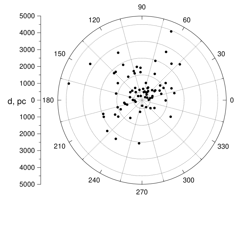
Figure 4: The distribution of the program Cepheids in the galactic plane

The galactocentric distance of the Sun R_G,⊙ = 7.9 kpc was adopted from the recent determination by McNamara et al. (mcnet00 (2000)). Estimated distances and other useful characteristics of our program Cepheids are gathered in Table 3. Because our spectra were obtained with different spectrographs having differing resolving powers, and also because for different stars we have a differing number of spectra (as a rule, one spectrum for Cepheids observed with 6-m telescope), we have assigned for each star a weight in the derivation of the gradient solution. We assigned a weight W = 1 to the following stars: those observed with the 6-m telescope (lower resolution spectra), the two stars observed by Harris & Pilachowski (hp84 (1984)), and the stars with one high resolution spectrum, but a low S/N ratio (VX Pup, CV Mon and MY Pup). For the rest of the program stars a weight W = 3 was used. The weights are given in the last column of Table 3. The distribution of the analyzed Cepheids in the galactic plane is shown in Fig. 4.

Table 3: Some physical and positional characteristics of program Cepheids

Star	P, d	$<$B-V$>$	E(B-V)	Mv	d, pc	l	b	RG, kpc	$<$[Fe/H]$>$	W
V473 Lyr (s)	2.6600	0.632	0.026	–2.47	517.2	60.56	7.44	7.66	–0.06	3
SU Cas (s)	2.7070	0.703	0.287	–2.49	322.7	133.47	8.52	8.12	–0.01	3
EU Tau (s)	2.9200	0.664	0.172	–2.58	1058.2	188.80	–5.32	8.94	–0.06	3
IR Cep (s)	2.9360	0.870	0.411	–2.59	624.4	103.40	4.91	8.07	–0.01	1
TU Cas	2.1393	0.582	0.115	–2.21	821.4	118.93	–11.40	8.32	+0.03	3
DT Cyg (s)	3.4720	0.538	0.039	–2.79	487.4	76.55	–10.78	7.80	+0.11	3
V526 Mon (s)	3.7150	0.593	0.093	–2.87	1716.6	215.13	1.81	9.36	–0.13	1
V351 Cep (s)	3.8970	0.940	0.400	–2.93	1640.5	105.20	–0.72	8.48	+0.03	1
VX Pup	3.0109	0.610	0.136	–2.62	1265.5	237.02	–1.30	8.65	–0.13	1
SZ Tau (s)	4.3730	0.844	0.294	–3.07	536.5	179.48	–18.74	8.41	+0.08	3
V1334 Cyg(s)	4.6290	0.504	0.000	–3.14	633.2	83.60	–7.95	7.85	–0.04	3
BG Cru (s)	4.6430	0.606	0.053	–3.14	491.2	300.42	3.35	7.66	–0.02	3
BD Cas (s)	3.6510	–	0.734	–3.25	2371.5	118.00	–0.96	9.25	–0.07	1
RT Aur	3.7282	0.595	0.051	–2.88	428.2	183.15	8.92	8.32	+0.06	3
DF Cas	3.8328	1.181	0.599	–2.91	2297.9	136.00	1.53	9.68	+0.13	1
SU Cyg	3.8455	0.575	0.096	–2.91	781.5	64.76	2.50	7.60	–0.00	3
ST Tau	4.0343	0.847	0.355	–2.97	1020.7	193.12	–8.05	8.89	–0.05	3
V1726 Cyg(s)	5.8830	0.885	0.312	–3.43	1916.2	92.50	–1.61	8.21	–0.02	1
BQ Ser	4.2709	1.399	0.841	–3.04	911.7	35.13	5.37	7.18	–0.04	3
Y Lac	4.3238	0.731	0.217	–3.05	1996.6	98.72	–4.03	8.43	–0.09	3
T Vul	4.4355	0.635	0.064	–3.09	532.7	72.13	–10.15	7.76	+0.01	3
FF Aql (s)	6.2100	0.756	0.224	–3.49	424.4	49.20	6.36	7.63	+0.02	3
CF Cas	4.8752	1.174	0.566	–3.20	3145.2	116.58	–0.99	9.72	–0.01	3
TV Cam	5.2950	1.198	0.644	–3.30	3739.1	145.02	6.15	11.15	–0.06	1
BG Lac	5.3319	0.949	0.336	–3.31	1656.6	92.97	–9.26	8.15	–0.01	3
Del Cep	5.3663	0.657	0.092	–3.31	247.9	105.19	0.53	7.97	+0.06	3
V1162 Aql(s)	7.4670	0.900	0.205	–3.71	1470.2	29.40	–18.60	6.72	+0.01	3
CV Mon	5.3789	1.297	0.714	–3.32	1809.1	208.57	–1.79	9.53	–0.03	1
V Cen	5.4939	0.875	0.289	–3.34	702.3	316.40	3.31	7.41	+0.04	3
V924 Cyg	5.5710	0.847	0.258	–3.36	4428.4	66.90	5.33	7.38	–0.09	1
MY Pup (s)	7.9100	0.631	0.064	–3.78	708.4	261.31	–12.86	8.03	–0.12	1
Y Sgr	5.7734	0.856	0.205	–3.40	496.1	12.79	–2.13	7.42	+0.06	3
EW Sct	5.8233	1.725	1.128	–3.41	345.0	25.34	–0.09	7.59	+0.04	3
FM Aql	6.1142	1.277	0.646	–3.47	842.3	44.34	0.89	7.32	+0.08	3
TX Del	6.1660	0.766	0.132	–3.48	2782.5	50.96	–24.26	6.60	+0.24	3
V367 Sct	6.2931	1.769	1.130	–3.51	1887.7	21.63	–0.83	6.18	–0.01	3
X Vul	6.3195	1.389	0.848	–3.51	831.6	63.86	–1.28	7.57	+0.08	3
AW Per	6.4636	1.055	0.534	–3.54	724.9	166.62	–5.39	8.60	+0.01	3
U Sgr	6.7452	1.087	0.403	–3.59	620.5	13.71	–4.46	7.30	+0.04	3
V496 Aql (s)	9.4540	1.146	0.413	–4.00	1195.1	28.20	–7.13	6.88	+0.05	3
Eta Aql	7.1767	0.789	0.149	–3.66	260.1	40.94	–13.07	7.71	+0.05	3
BB Her	7.5080	1.100	0.414	–3.72	3091.7	43.30	6.81	6.04	+0.15	3
RS Ori	7.5669	0.945	0.389	–3.73	1498.9	196.58	0.35	9.35	–0.10	3
V440 Per (s)	10.5140	0.873	0.273	–4.12	801.1	135.87	–5.17	8.49	–0.05	3
W Sgr	7.5949	0.746	0.111	–3.73	405.4	1.58	–3.98	7.50	–0.01	3
RX Cam	7.9120	1.193	0.569	–3.78	833.4	145.90	4.70	8.60	+0.03	3
W Gem	7.9138	0.889	0.283	–3.78	916.9	197.43	3.38	8.78	–0.04	3
U Vul	7.9906	1.275	0.654	–3.79	570.9	56.07	–0.29	7.60	+0.05	3
DL Cas	8.0007	1.154	0.533	–3.79	1602.1	120.27	–2.55	8.82	–0.01	3
AC Mon	8.0143	1.165	0.508	–3.80	2754.8	221.80	–1.86	10.12	–0.07	1
V636 Cas (s)	11.6350	1.391	0.786	–4.25	592.2	127.50	1.09	8.27	+0.06	3
S Sge	8.3821	0.805	0.127	–3.85	648.1	55.17	–6.12	7.55	+0.10	3
GQ Ori	8.6161	0.976	0.279	–3.88	2437.6	199.77	–4.42	10.22	–0.03	1
V500 Sco	9.3168	1.276	0.599	–3.98	1406.1	359.02	–1.35	6.49	–0.02	3
FN Aql	9.4816	1.214	0.510	–4.00	1383.2	38.54	–3.11	6.87	–0.02	3
YZ Sgr	9.5536	1.032	0.292	–4.01	1205.4	17.75	–7.12	6.77	+0.05	3
S Nor	9.7542	0.941	0.215	–4.03	879.6	327.80	–5.39	7.17	+0.05	3
Beta Dor	9.8424	0.807	0.044	–4.04	335.8	271.73	–32.78	7.90	–0.01	3
Zeta Gem	10.1507	0.798	0.018	–4.08	387.2	195.75	11.90	8.27	+0.04	3
Z Lac	10.8856	1.095	0.404	–4.17	1782.4	105.76	–1.62	8.56	+0.01	3
VX Per	10.8890	1.158	0.515	–4.17	2283.5	132.80	–2.96	9.60	–0.05	3
V340 Nor(s:)	11.2870	1.149	0.332	–4.21	1976.1	329.80	–2.23	6.27	+0.00	3
RX Aur	11.6235	1.009	0.276	–4.24	1579.0	165.77	–1.28	9.44	–0.07	3
TT Aql	13.7547	1.292	0.495	–4.45	976.1	36.00	–3.14	7.13	+0.11	3
SV Mon	15.2328	1.048	0.249	–4.57	2472.3	203.74	–3.67	10.21	–0.03	3
X Cyg	16.3863	1.130	0.288	–4.66	1043.5	76.87	–4.26	7.73	+0.12	3
RW Cam	16.4148	1.351	0.649	–4.66	1748.4	144.85	3.80	9.38	+0.04	3
CD Cyg	17.0740	1.266	0.514	–4.71	2462.1	71.07	1.43	7.47	+0.07	3
Y Oph (s)	23.7880	1.377	0.655	–5.11	664.9	20.60	10.12	7.29	+0.05	3
SZ Aql	17.1408	1.389	0.641	–4.71	1731.0	35.60	–2.34	6.57	+0.15	3
YZ Aur	18.1932	1.375	0.565	–4.78	4444.7	167.28	0.94	12.27	–0.05	1
WZ Sgr	21.8498	1.392	0.467	–5.00	1967.5	12.11	–1.32	5.99	+0.17	3
SW Vel	23.4410	1.162	0.349	–5.09	2572.4	266.20	–3.00	8.47	+0.01	3
X Pup	25.9610	1.127	0.443	–5.21	2776.6	236.14	–0.78	9.72	–0.03	3
T Mon	27.0246	1.166	0.209	–5.26	1369.7	203.63	–2.55	9.17	+0.13	3
SV Vul	44.9948	1.442	0.570	–5.87	1729.5	63.95	0.32	7.31	+0.03	3
S Vul	68.4640	1.892	0.827	–6.38	3199.7	63.45	0.83	7.07	–0.02	3

6 Results and discussion

6.1 The radial distribution of elemental abundances: general picture and remarks on some elements

Using our calculated galactocentric distances and average abundances we can determine the galactic metallicity gradient from a number of species. Plots for several chemical elements and results of a linear fit are given in Fig. 5 (iron) and Figs. 6-9 (other elements). Note that, in the plots for Si and Cr, TX Del is not included. This star shows rather strong excess in the abundances of these elements which could be connected with its peculiar nature (in Harris & Welch hw89 (1989) TX Del is reported as a spectroscopic binary. It has also been labeled a Type II Cepheid at times). In the plot for carbon we did not include the data for FN Aql and SV Mon, both of which have an extremely low carbon abundances. These two unusual Cepheids will be discussed in detail in a separate paper.

The information in the plots and also in Fig. 10 enables one to put together several important conclusions. Most radial distributions of the elements studied indicate a negative gradient ranging from about $-0.02$ dex kpc^-1 to $-0.06$ dex kpc^-1, with an average of $-0.03$ dex kpc^-1 for the elements in Figs. 5-8. The most reliable value comes from iron (typically the number of iron lines for each star is about 200-300). The gradient in iron is $-0.029$ dex kpc^-1, which is close to the typical gradient value produced by other iron-group elements. Examination of Fig. 5 might lead one to suspect that the iron gradient is being controlled by the cluster of stars at R $\approx 6.5$ with [Fe/H] $\approx 0.2$. If one deletes these stars from the solution the gradient falls to approximately $-0.02$ dex kpc^-1. This latter value differs from the value determined using all the data by about twice the formal uncertainty in either slope. However, we do not favour the neglect these points as there is no reason to suspect these abundances relative to the bulk of the objects. Indeed, in a subsequent paper, we shall present results for Cepheids which lie closer to the galactic center and which have abundances above those of this study, which may imply a steepening of the gradient towards the galactic center.

Unweighted iron abundances give a gradient of $-0.028$ dex kpc^-1. Both weighted and unweighted iron gradients are not significantly changed if we remove two Cepheids at galactocentric distances greater than 11 kpc (gradient is $-0.031$ dex kpc^-1). Thus, the average slope of about $-0.03$ dex kpc^-1 probably applies to the range $6\leq$ R_G (kpc) $\leq 10$. Notice that in all cases the correlation coefficient is relatively low, r $\approx 0.47$.

Carbon shows a surprisingly clear dependence upon galactocentric distance (Fig. 6a): the slope of the relation is among the largest from examined elements. We have included in the present study elements such as carbon and sodium, although the gradients based on their abundances determined from Cepheids may not be conclusive. In fact, it is quite likely that the surface abundances of these elements have been altered in these intermediate mass stars during their evolution from the main sequence to the Cepheid stage. For example, the surface abundance of carbon should be decreased after the global mixing which brings the CNO-processed material into the stellar atmosphere (turbulent diffusion in the progenitor B main sequence star, or the first dredge-up in the red giant phase). Some decrease in the surface abundance of oxygen is also expected for supergiant stars, but at a significantly lower level than for carbon (Schaller et al. schallet92 (1992)).

It is also well known that galactic supergiants (Cepheids, in particular) show an increased sodium abundance which is usually interpreted as a result of dredge-up of material processed in the Ne–Na cycle (and therefore enriched in sodium) to the stellar surface (Sasselov sass86 (1986), Luck luck94 (1994), Denissenkov 1993a , 1993b , denis94 (1994)). Such a contamination of the Cepheids’ atmospheres with additional sodium may result in a bias of the [Na/H] gradient value derived from Cepheids in relation to the true gradient. It can be seen that our results in Fig. 6a,c are consistent with these considerations on C and Na, respectively. It is not clear how these effects should affect stars at different galactocentric distances (with different metallicities), but it is likely that they contribute to increase the dispersion in the abundances, thus producing a flatter gradient.

There are some indications (Andrievsky & Kovtyukh ankov96 (1996)) that surface Mg and Al abundances in yellow supergiants can be altered to some extent due to mixing of the material processed in the Mg–Al cycle with atmospheric gas. This supposition seems to gain some additional support from our present data (see Fig.11) where one can see that the Mg and Al abundances are correlated.

As surface abundance modifications depend upon the number of visits to the red giant region (i.e. the number of dredge-up events) as well as other factors (pre dredge-up events, depth of mixing events, mass), it is possible that the program Cepheids could show differential evolutionary effects in their abundances. Because of the high probability of such effects impacting the observed carbon and sodium (and perhaps, oxygen, magnesium, and aluminum) abundances in these Cepheids, we recommend that our gradient values for carbon and sodium to be viewed with extreme caution, while the gradients of oxygen, magnesium and aluminum abundances could be used, but also with some caution.

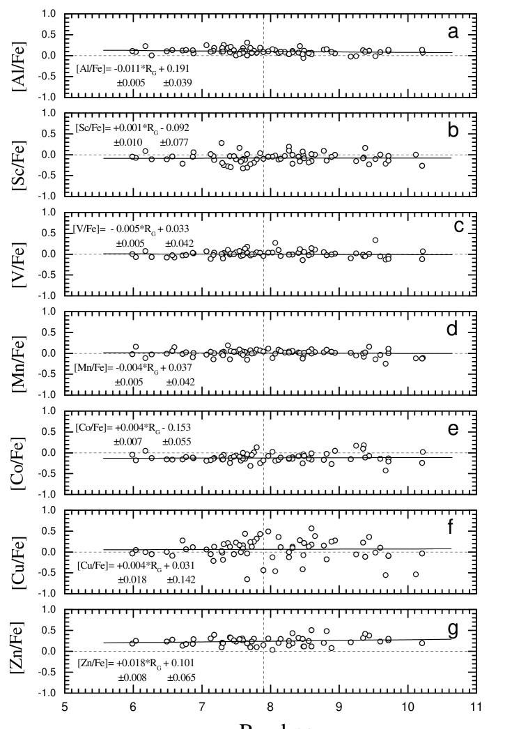
Figure 12: Gradients for some abundance ratios

The difference in metallicity between the stars of our sample (say, at 6 kpc and 10 kpc) is about 0.25 dex. This is a rather small value to detect/investigate the so-called ”odd-even” effect, that is the metallicity dependent yield for some elements which should be imprinted on the trends of abundance ratios for [El_odd/El_even] versus galactocentric distance, see for details Hou, Prantzos & Boissier (hpb00 (2000)). Such elements as, for example, aluminum, scandium, vanadium and manganese should show progressively decreasing abundances with overall metal decrease. This should manifest itself as a gradient in [El_odd/Fe]. We have plotted the abundance ratios for some ”odd” elements (normalized to iron abundance) versus R_G in Fig.12. As one can see, none of the abundance ratios plotted versus galactocentric distance shows a clear dependence upon R_G. This could mean that the ”odd-even” effect may be overestimated if only the yields from massive stars are taken into account ignoring other possible sources, or that the effect is not sufficiently large to be seen over the current distance and metallicity baseline.

6.2 Metallicity dispersion and the metallicity in the solar vicinity

There is a spread in the metallicity at each given galactocentric distance (larger than the standard error of the abundance analysis) which is most likely connected with local inhomogeneities in the galactic disc. As an example, in Fig. 13, we show the derived iron abundance vs. galactic longitude for the stars of our sample (a few Cepheids with heliocentric distances large than 3000 pc were excluded). The distribution gives only a small hint about a local increase of the metallicity in the solar vicinity towards the direction l$\approx 30^{\degr}$ and $150^{\degr}$.

It is important to note that at the solar galactocentric distance those elements, whose abundance is not supposed to be changed in supergiants during their evolution, show on average the solar abundance in Cepheids. Relative to the solar region, the stars within our sample which are within 500 pc of the Sun have a mean [Fe/H] of $\approx+0.01$ (n = 14, $\sigma=0.06$). If we consider all program stars at a galactocentric radius of 7.4–8.4 kpc, i.e. those in a 1 kpc wide annulus centered at the solar radius, we find a mean [Fe/H] of approximately +0.03 (n = 29, $\sigma=0.05$).

This result again stresses the importance of the problem connected with subsolar metallicities reported for the hot stars from the solar vicinity (see, e.g. Gies & Lambert gila92 (1992), Cunha & Lambert cunla94 (1994), Kilian kil92 (1992), Kilian, Montenbruck & Nissen kmn94 (1994), Daflon, Cunha & Becker dafcube99 (1999), Andrievsky et al. anet99 (1999)). This also follows from the plots provided by Gummersbach et al. (guet98 (1998)) for several elements.

This problem was discussed, for instance, by Luck et al. (lucket00 (2000)). The authors compared the elemental abundances of B stars from the open cluster M25 with those of the Cepheid U Sgr and two cool supergiants which are also members of the cluster, and found disagreement in the abundances of the B stars and supergiants; e.g., while the supergiants of M25 show nearly solar abundances, the sample of B stars demonstrate a variety of patterns from under- to over-abundances. This should not be observed if we assume that all stars in the cluster were born from the same parental nebula. Obviously, the problem of some disagreement between abundance results from young supergiants and main-sequence stars requires further investigation.

6.3 Flattening of the elemental distribution in the solar neighbourhood

All previous studies of the radial abundance distribution in the galactic disc have considered only chemical elements from carbon to iron, and all derived gradients have shown a progressive decrease in abundance with increasing galactocentric distance. For the elements from carbon to yttrium in this study our gradient values also have negative signs, while for the heavier species (from zirconium to gadolinium) we obtained (within the error bars) near-to-zero gradients (see Fig. 10). Two obvious features which are inherent to derived C-Gd abundance distributions have to be interpreted: a rather flat character of the distribution for light/iron-group elements, and an apparent absence of a clear gradient for heavy species.

The flattening of the abundance distribution can be caused by radial flows in the disc which may lead to a homogenization of ISM. Among the possible sources forcing gas of ISM to flow in the radial direction, and therefore producing a net mixing effect there could be a gas viscosity in the disc, gas infall from the halo, gravitational interaction between gas and spiral waves or a central bar (see e.g., Lacey & Fall lf85 (1985) and Portinari & Chiosi pch00 (2000)).

The mechanism of the angular momentum re-distribution in the disc based on the gas infall from the halo is dependent upon the infall rate, and therefore it should have been important at the earlier stages of the Galaxy evolution, while other sources of the radial flows should effectively operate at present.

Gravitational interaction between the gas and density waves produces the radial flows with velocity (Lacey & Fall lf85 (1985)):

$$v_{\rm r}\sim(\Omega_{\rm p}-\Omega_{\rm c})^{-1},$$ (4)

where $\Omega_{\rm p}$ and $\Omega_{\rm c}$ are the angular velocities of the spiral wave and the disc rotation respectively. According to Amaral & Lépine (amle97 (1997)) and Mishurov et al. (miet97 (1997)) among others, based on several different arguments, the galactic co-rotation resonance is located close to the solar galactic orbit. The co-rotation radius is the radius at which the galactic rotation velocity coincides with the rotation velocity of the spiral pattern. Together with Eq. (4) this means that, inside the co-rotation circle, gas flows towards the galactic center ($\Omega_{\rm c}>\Omega_{\rm p}$ and v${}_{\rm r}<0$), while outside it flows outwards. This mechanism can produce some ”cleaning” effect in the solar vicinity, and thus can lead to some flattening of the abundance distribution. In addition, it could explain the similarity in the solar abundances and mean abundances in the five billion years younger Cepheids located at the solar galactocentric annulus (see Fig. 5), although one might expect that the Cepheids from this region should be more abundant in metals than our Sun.

There is a clear evidence that the bars of spiral galaxies have also a great impact on chemical homogenization in the discs (Edmunds & Roy er93 (1993); Martin & Roy mr94 (1994), Gadotti & Dos Anjos gda01 (2001)). It has been shown that a flatter abundance gradient is inherent to galaxies which have a bar structure. This could imply that a rotating bar is capable of producing significant homogenization of the interstellar medium, while such homogenization is not efficient in unbarred spiral galaxies.

The direct detection of a bar at the center of our galaxy using $COBE$ maps was reported by Blitz & Spergel (bs91 (1991)). Kuijken (kui96 (1996)), Gerhard (ger96 (1996)), Gerhard, Binney & Zhao (geret98 (1998)), Raboud et al. (rabet98 (1998)) also suggest that the Milky Way is a barred galaxy. The most recent evidence for a long thin galactic bar was reported by López-Corredoira et al. (lcet01 (2001)) from the DENIS survey. These authors conclude that our Galaxy is a typical barred spiral. If so, then the Milky Way should obey the relation between the slope of metallicity distribution and the bar strength (specifically, the axial ratio), which is based on the data obtained from other galaxies.

According the above mentioned authors the galactic bar is triaxial and has an axial ratio (b/a) of about $1/3-1/2$ (see also Fux fux97 (1997), fux99 (1999)). With such axial ratio an ellipticity E_B = 10 (1-b/a) $\approx 5-7$. Lépine & Leroy (ll00 (2000)) presented a model which reproduces a near-infrared brightness distribution in the Galaxy. Their estimate of the galactic bar characteristics supposes that the total length of the bar should be about 4.6 kpc, while its width about 0.5 kpc. In this case an ellipticity could be even larger than 7. For such ellipticities the observational calibration of Martin & Roy (mr94 (1994)) for barred galaxies predicts a metallicity slope of about $-0.03$ to $\approx 0$ dex kpc^-1 for oxygen. Our results on abundance gradients in the solar neighbourhood for iron-group elements and light species (such as Si, Ca, and even oxygen) appear to be in good agreement with expected gradient value which is estimated for the galactic disc solely from bar characteristics.

Martinet & Friedli (mf97 (1997)) investigated secular chemical evolution in barred systems and found that a strong bar is capable of producing significant flattening of the initial gradient across the disc. Using numerical results of that paper one can trace the (O/H) abundance evolution in barred systems. With our abundance gradients for such elements as oxygen, silicon, calcium and iron-group elements one can conclude that an expected age of the galactic bar is approximately 1 Gyr, or less. Another important result obtained by Martinet & Friedli (mf97 (1997)) is that the bar of such an age should produce not only significant flattening across almost the whole disc, but also steepening of the abundance distribution in the inner parts (our observational results for this region will be discussed in the next paper from this series).

An additional mechanism which may cause some local flattening (or even a shallow local minimum in the elemental abundances) should operate near the galactocentric solar radius where the relative rotational velocity of the disc and spiral pattern is small. The shocks that arise when the gas orbiting in the disc penetrates the spiral potential perturbation, and which are responsible for triggering star formation in spiral arms, pass through a minimum strength at this galactic radius, due to almost zero relative velocity. Furthermore, simulations performed by Lépine, Mishurov & Dedikov (lmd01 (2001)) show that there is also a gas depletion at the co-rotation radius. Both reasons point towards a minimum of star formation rate at the co-rotation radius. This lower star formation rate manifests itself in the models as a minimum in elemental abundances. One can expect that after a few billion years, a galactic radius with minimum star formation rate should correspond to a local minimum in metallicity. The flat local minimum in metal abundance should be observable, unless the mechanisms that produce radial transport or radial mixing of the gas in the disc are important, or if the co-rotation radius varied appreciably in a few billion years. Note that the star-formation rate also depends on the gas density, which decreases towards large galactic radii. The combined effect of gas density and co-rotation could produce a slightly displaced minimum.

At first glance, the abundance data presented in Figs. 5-9 show little indication of a local abundance minimum (or discontinuity) at the solar galactocentric radius. Nevertheless, the parabolic fit of the iron abundance distribution rather well represents observed data, and shows that a small increase in the metallicity at galactic radii larger than the co-rotation radius may not be excluded (Fig. 14).

Comparing gradients from iron-group elements (small and negative) with those from the heaviest species (near to zero) one could propose the following preliminary explanation of the observed difference. The known contributors of the O-to-Fe-peak nuclei to ISM are massive stars exploding as SNe II (short-lived) and SNe I (long-lived), while s-process elements (past iron-peak) are created only in the low-mass AGB stars (1-4 M_⊙, Travaglio et al. travet99 (1999)). The extremely flat distribution in the disc seen for s-process elements implies that there should exist some mechanism(s) effectively mixing ISM at time-scales less than the life times of the stars with masses 1-4 M_⊙ ($\tau\approx 0.3-10$ Gyr). At the same time such a mechanism may not be able to completely erase the O-Fe gradients related to the ISM, and imprinted on the young stars. If the characteristic time of the mixing (even being possibly comparable to the SNe I life time) exceeds a nuclear evolution of the SNe II O-Fe contributors, then these are the high-mass stars that could be responsible for the resulting small negative gradients from O-Fe elements in the disc.

If one adopts the velocity of the radial flows, say, 4 km s^-1 (see discussion in Lacey & Fall lf85 (1985) and Stark & Brand stbr89 (1989)), then the necessary time to mix the gas within about 4 kpc (baseline covered by our data) should be likely less than 1 Gyr, that is below the life-time intervals for AGB progenitors with 1-2 M_⊙. However, this $ad\leavevmode\nobreak\ hoc$ supposition meets a problem with the observed Eu gradient. This element is believed to be produced mainly through the r-process in lower-mass SNe II (e.g., Travaglio et al. travet99 (1999)), and therefore should probably behave similar to, for example, iron, but its radial abundance distribution appears to be quite similar to that of the s-process elements, like Zr, La, Ce, Nd (see Fig. 10).

Figure 1: Program Cepheid gravities vs. their pulsational periods

Figure 2: Relative-to-solar Ce and Eu abundance and spectroscopic gravity of U Sgr vs. its pulsational phases

Figure 3: Same as Fig. 2 but for SV Vul

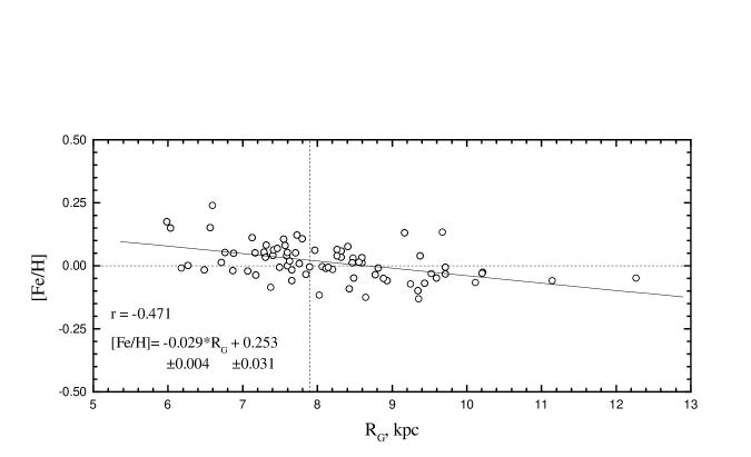
Figure 5: Iron abundance gradient and its linear approximation. The position of the Sun is at the intersection of the dashed lines

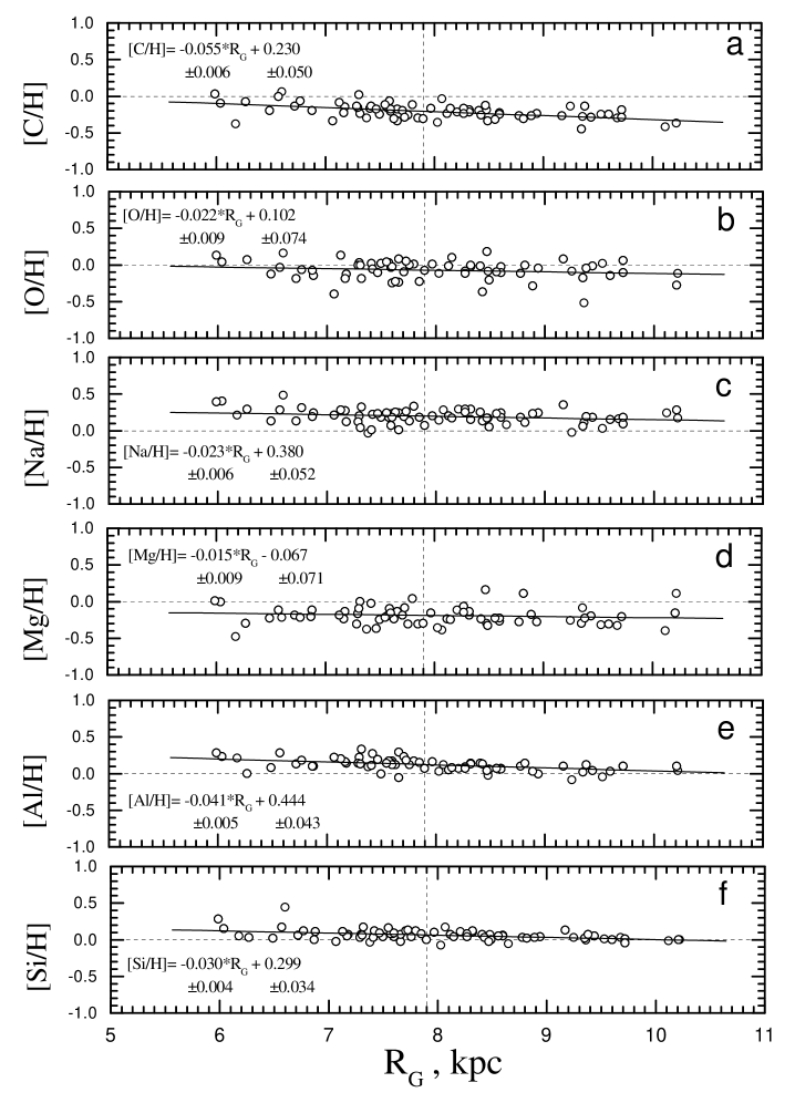
Figure 6: Abundance gradients for other investigated elements: C–Si

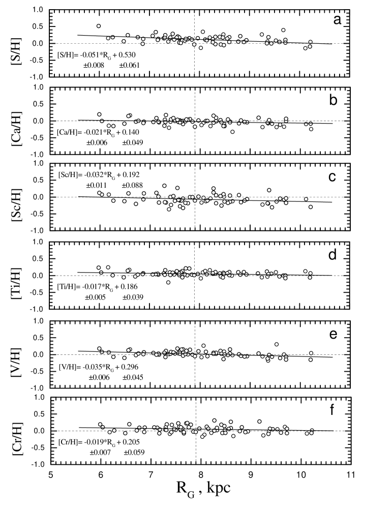
Figure 7: Same as Fig.6, but for S–Cr

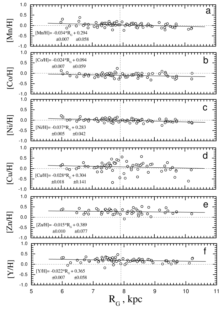
Figure 8: Same as Fig.6, but for Mn–Y

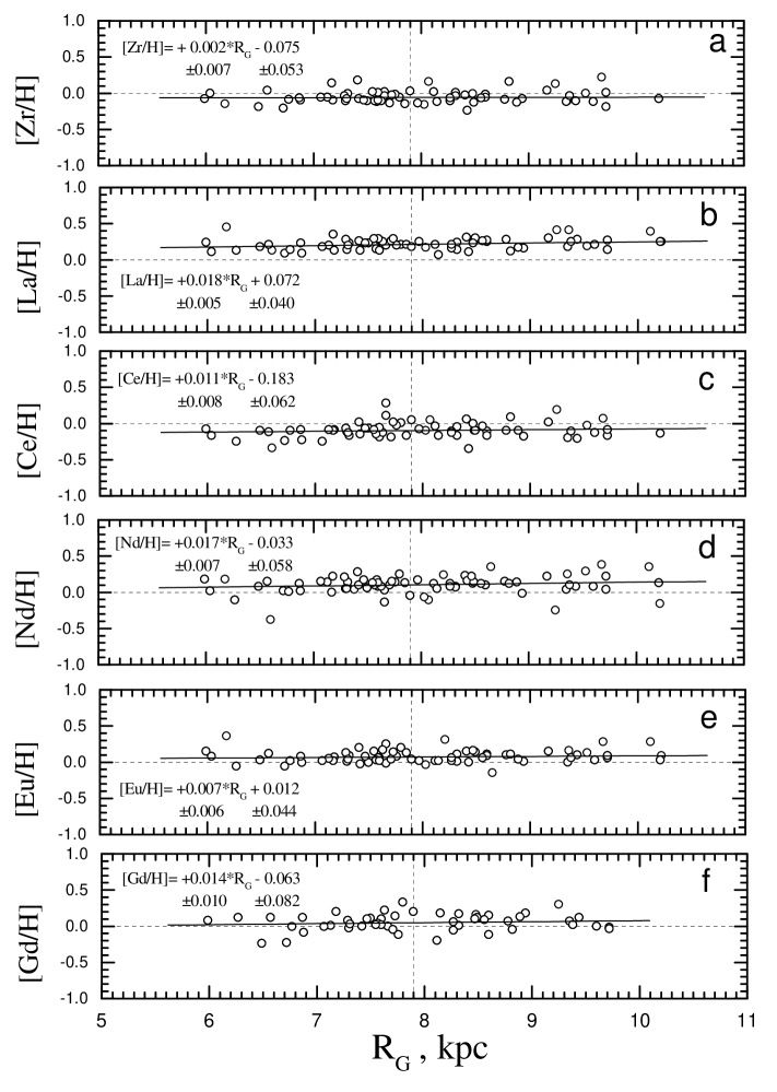
Figure 9: Same as Fig.6, but for Zr–Gd

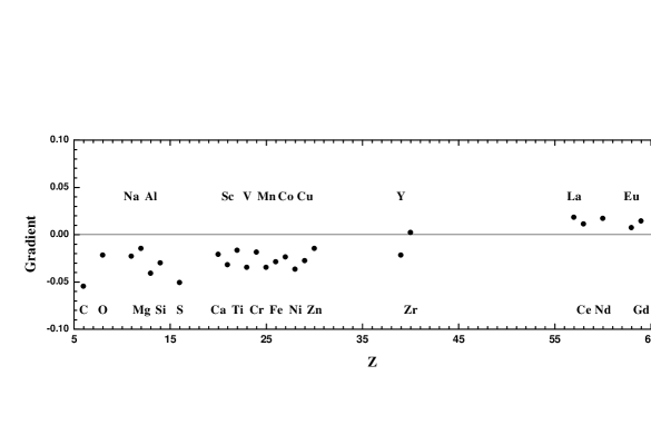
Figure 10: Derived gradients versus atomic number

Figure 11: [Al/H] vs. [Mg/H] for program Cepheids

Figure 13: Iron abundance vs. galactic longitude

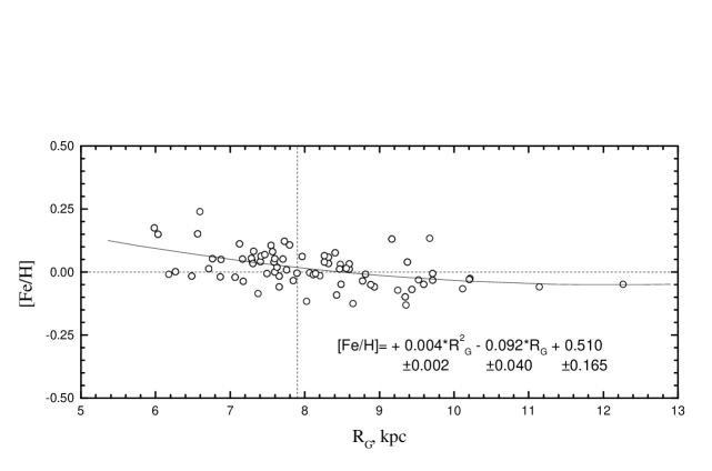
Figure 14: Iron abundance profile with a parabolic approximation

- (1) Afflerbach A., Churchwell E., Werner M.W., 1997, ApJ 478, 190
- (2) Amaral L.H., Lépine J.R.D., 1997, MNRAS 286, 885
- (3) Andrievsky S.M., Kovtyukh V.V., 1996, Ap&SS 245, 61
- (4) Andrievsky S.M., Kovtyukh V.V., Bersier D., Luck R.E., Gopka V.F., Yushchenko A.V., Usenko I.A., 1998, A&A 329, 599
- (5) Andrievsky S.M., Korotin S.A., Luck, R. E., Kostynchuk, L.Yu., 1999, A&A 342, 756
- (6) Andrievsky S.M., Kovtyukh V.V., Korotin S.A., Spite M., Spite F., 2001, A&A 367, 605
- (7) Barklem P. S., Piskunov N., O’Mara B. J., 2000, A&A 142, 467
- (8) Blitz L., Spergel D.N., 1991, ApJ 379, 631
- (9) Cameron L.M., 1985, A&A 147, 47
- (10) Carraro G., Ng Yu.K., Portinari L., 1998, MNRAS 296, 1045
- (11) Castelli F., 1996, ASP Conf. Ser. 108, Model atmospheres and stellar spectra, S.J. Adelman, F. Kupka, W.W. Weiss (Eds.), San Francisco, 85
- (12) Christensen-Dalsgaard , Petersen J.O., 1995, A&A 299, L17
- (13) Cunha K., Lambert D.L., 1994, ApJ 426, 170
- (14) Daflon S., Cunha K., Becker S.R., 1999, ApJ 522, 950
- (15) Deharveng L., Peña M., Caplan J., Costero R., 2000, MNRAS 311, 329
- (16) Dennisenkov P. A., 1993a, SSR 66, 405
- (17) Dennisenkov P. A., 1993b, SSR 74, 363
- (18) Dennisenkov P. A., 1994, A&A 287, 113
- (19) Edmunds M.G., Roy J.-R., 1993, MNRAS 261, L17
- (20) Evans N.R., Teays T.J., 1996, AJ 112, 761
- (21) Fernie J.D., Evans N.R., Beattie B., Seager S., 1995, IBVS 4148, 1
- (22) Fernley J.A., Skillen I., Jameson R.F., 1989, MNRAS 237, 947
- (23) Fich M., Silkey M., 1991, ApJ 366, 607
- (24) Fitzsimmons A., Brown P.J.F., Dufton P.L., Lennon D.J., 1990, A&A 232, 437
- (25) Fitzsimmons A., Dufton P.L., Rolleston W.R.J., 1992, MNRAS, 259, 489
- (26) Friel E.D., 1995, ARA&A 33, 381
- (27) Friel E.D., 1999, Ap&SS 265, 271
- (28) Friel E.D., Janes K.A., 1993, A&A 267, 75
- (29) Fry A.M., Carney B.W., 1997, AJ 113, 1073
- (30) Fux R., 1997, A&A 327, 983
- (31) Fux R., 1999, A&A 345, 787
- (32) Gadotti D.A., Dos Anjos S., 2001, ApJ, in press
- (33) Gehren T., Nissen P.E., Kudritzki R.P., Butler K., 1985, Proc. ESO Workshop on production and distribution of CNO elements, Eds. I.J. Danziger, F. Matteucci, K. Kjaer, Garching, ESO, 171
- (34) Geisler D., Clariá J.J., Minniti D., 1992, AJ 104, 1892
- (35) Gerhard O.E., 1996, Unresolved problems of the Milky Way, Blitz L., Teuben P. (Eds.), Kluwer, Dordrecht, 79
- (36) Gerhard O.E., Binney J.J., Zhao H., 1998, Highlights of Astronomy, Andersen J. (Ed.), Kluwer, Dordrecht, 628
- (37) Gieren W.P., Fouqué P., Gómez M., 1998, ApJ 496, 17
- (38) Gies D.R., Lambert D.L., 1992, ApJ 387, 673
- (39) Gough D.O., Ostriker J.P., Stobie R.S., 1965, ApJ 142, 1649
- (40) Grevesse N., Noels A., Sauval J., 1996, ASP Conf. Ser. 99, 117
- (41) Gummersbach C.A., Kaufer D.R., Schäfer D.R., Szeifert T., Wolf B., 1998, A&A 338, 881
- (42) Harris H.C., 1981, AJ 86, 707
- (43) Harris H.C., Pilachowski C.A., 1984, ApJ 282, 655
- (44) Harris H.C., Welch D.L., 1989, AJ 98, 981
- (45) Hill V., Andrievsky S.M., Spite M., 1995, A&A 293, 347
- (46) Hou J.L., Prantzos N., Boissier S., 2000, A&A 362, 921
- (47) Janes K.A., 1979, ApJS 39, 135
- (48) Kaufer A., Szeifert T., Krenzin R., Baschek B., Wolf B., 1994, A&A 289, 740
- (49) Kilian J., 1992, A&A 262, 171
- (50) Kilian J., Montenbruck O., Nissen P.E., 1994, A&A 284, 437
- (51) Kilian-Montenbruck J., Gehren T., Nissen P.E., 1994, A&A 291, 757
- (52) Kiss L.L., 1998, MNRAS 297, 825
- (53) Kovtyukh V.V., Andrievsky S.M., 1999, A&A 351, 597
- (54) Kovtyukh V.V., Gorlova N.I., 2000, A&A 358, 587
- (55) Kuijken K., 1996, Barred galaxies, Buta R., Crocker D.A., Elmegreen B.G. (Eds.), ASP, San Francisco, 504
- (56) Kurucz R.L. 1992, The Stellar Populations of Galaxies, Eds. B. Barbuy, A. Renzini, IAU Symp. 149, 225
- (57) Kurucz R.L., Furenlid I., Brault I., Testerman L., 1984, The solar flux atlas from 296 nm to 1300 nm, NSO
- (58) Lacey C.G., Fall M., 1985, ApJ 290, 154
- (59) Laney C.D., Stobie R.S., 1993, MNRAS 263, 291
- (60) Lépine J.R.D., Leroy P., 2000, MNRAS 313, 263
- (61) Lépine J.R.D., Mishurov Yu.N., Dedikov S.Yu., 2001, ApJ 546, 234
- (62) López-Corredoira M., Hammersley P.L., Garzón F., Cabrera-Lavers A., Castro-Rodriguez N., Schultheis M., Mahoney T.J., 2001, A&A 373, 139
- (63) Luck R.E., 1982, ApJ 256, 177
- (64) Luck R.E., 1994, ApJS 91, 309
- (65) Luck R.E., Andrievsky S.M., Kovtyukh V.V., Korotin S.A., Beletsky Yu.V., 2000, A&A 361, 189
- (66) Maciel W.J., Köppen J., 1994, A&A 282, 436
- (67) Maciel W.J., Quireza C., 1999, A&A 345, 629
- (68) Martin P., Roy J.-R., 1994, ApJ 424, 599
- (69) Martinet L., Friedli D., 1997, A&A 323, 363
- (70) McNamara D.H., Madsen J.B., Barnes J., Ericksen B.F., 2000, PASP 112, 202
- (71) Mishurov Yu.N., Zenina I.A., Dambis A.K., Mel’nik A.M., Rastorguev A.S., 1997, A&A 323, 775
- (72) Neese C.L., Yoss K.M., 1988, AJ 95, 463
- (73) Panagia N., Tosi M., 1981, A&A 96, 306
- (74) Pasquali A., Perinotto M., 1993, A&A 280, 581
- (75) Peña M., Deharveng L., Caplan J., Costero R., 2000, RevMexAA 9, 184
- (76) Phelps R., 2000, Chemical evolution of the Milky Way, F. Matteucci, F. Giovannelli (Eds.), Kluwer Dordrecht, 239
- (77) Portinari L., Chiosi C., 2000, A&A 355, 929
- (78) Raboud D., Grenon M., Martinet L., Fux R., Udry S., 1998, A&A 335, L61
- (79) Rodriguez M., 1999, A&A 351, 1075
- (80) Rolleston W.R.J., Smartt S.J., Dufton P.L., Ryans R.S.I., 2000, A&A 363, 537
- (81) Rudolph A.L., Simpson J.P., Haas M.R., Erickson E.F., Fich M., 1997, ApJ 489, 94
- (82) Sasselov D.D., 1986, PASP 98, 561
- (83) Schaller G., Shaerer D., Meynet G., Maeder A., 1992, A&AS 96, 269
- (84) Shaver P.A., McGee R.X., Newton L.M., Danks A.C., Pottasch S.R., 1983, MNRAS 204, 53
- (85) Simpson J.P., Rubin R.H., 1990, ApJ 354, 165
- (86) Simpson J.P., Colgan S.W.J., Rubin R.H., Erickson E.F., Haas M.R., 1995, ApJ 444, 721
- (87) Smartt S.J., Rolleston W.R.J., 1997, ApJ 481, L47
- (88) Stark A.A., Brand J., 1989, ApJ 339, 763
- (89) Thogersen E.N., Friel E.D., Fallon B.V., 1993, PASP 105, 1253
- (90) Travaglio C., Galli D., Gallino R., Busso M., Ferrini F., Straniero O., 1999, ApJ 521, 691
- (91) Turner D.G., 1996, JRASC 90, 82
- (92) Vilchez J.M., Esteban C., 1996, MNRAS 280, 720