Using Cepheids to determine the galactic abundance gradient.II. Towards the galactic center

Based on spectra obtained at the Anglo-Australian Observatory, we present a discussion of the metallicity of the galactic disc derived using Cepheids at galactocentric distances 4-6 kpc. Our new results together with previous gradient determination (Paper I) show that the overall abundance distribution within the galactocentric distances 4–11 kpc cannot by represented by a single gradient value. The distribution is more likely bimodal: it is flatter in the solar neighbourhood with a small gradient, and steepens towards the galactic center. The steepening begins at a distance of about 6.6 kpc.

1 Introduction

In our previous work (Andrievsky et al. 2002, hereafter Paper I) results on elemental abundance distributions in the galactic disc based on 236 high-resolution spectra of 77 classical Cepheids in the solar neighborhood (galactocentric distances from 6 kpc to approximately 10.5 kpc) were reported. We found that among the 25 studied chemical elements, those from carbon to yttrium show small negative gradients, while heavier species produce near-to-zero gradients. Typical gradient values for iron-group elements were found to be equal to $\approx-0.03$ dex kpc^-1.

In order to extend our previous study and to check the behavior of the elemental distribution towards the galactic center we have observed several Cepheids with galactocentric distances between 4-6 kpc. In this work we present the results from these stars and discuss them together with the data from Paper I.

2 Observations

The spectra of the program stars (see Table 1) have been obtained on June 2nd 2001 at the Anglo-Australian Telescope with the University College of London Echelle Spectrograph (UCLES). The detector is an MIT/Lincoln Lab CCD with 15 micron pixels (2048 x 4096 pixels). With a 31 line mm^-1 grating, the resolving power is approximately 80000. The signal-to-noise ratio for all spectra is greater than 100, and the total coverage is 5000-9000 Å. The spectra were processed with the help of the DECH20 package (Galazutdinov, 1992).

Table 1: Program stars and details of the observations

Star	V	UT	Exp. (s)	JD 2452063.	$\phi$
VY Sgr	11.51	14:43:52	1800	.1242	0.394
UZ Sct	11.31	15:15:51	1800	.1464	0.455
AV Sgr	11.39	14:11:58	1800	.1021	0.982
V340 Ara	10.16	13:43:09	900	.0768	0.167
KQ Sco	9.81	13:59:43	600	.0866	0.940

3 Parameters of program stars and elemental abundances

The methods applied for the determination of the atmosphere parameters and elemental abundances are the same as described in detail in Paper I, and will not be repeated here. In Tables 2 and 3 the derived parameters of the program stars and their elemental abundances are given. Note that in particular, for the iron abundance, the standard deviation of the abundances is about 0.1. Given the number of iron lines utilized (44 - 102) the standard error of the mean is about 0.01. Following the scheme adopted in Paper I, in the gradient plots we have assigned weight 3 for all the program stars except KQ Sco. The lines in the spectrum of this star show some asymmetry. This factor limits the number of possible equivalent width measurements and may produce larger errors in the analysis. A weight of 1 was assigned for this star.

Table 2: Atmosphere parameters for program stars

Star	$\phi$	Teff, K	$\log g$	Vt,  km s-1
VY Sgr	0.394	5144	1.25	3.30
UZ Sct	0.455	5127	1.50	3.30
AV Sgr	0.982	5875	1.75	4.90
V340 Ara	0.167	5472	1.50	4.00
KQ Sco	0.940	5058	1.10	5.70

Table 3: Elemental abundances

	VY Sgr			UZ Sct			AV Sgr			V340 Ara			KQ Sco
Ion	[M/H]	$\sigma$	N	[M/H]	$\sigma$	N	[M/H]	$\sigma$	N	[M/H]	$\sigma$	N	[M/H]	$\sigma$	N
C I	0.01	0.23	3	0.04	0.15	3	0.21	0.13	14	0.20	0.11	8	–0.02	–	1
N I	0.50	–	1	0.70	–	1	0.82	0.11	2	1.00	0.12	2	–	–	–
O I	0.18	0.19	2	0.49	0.21	5	0.36	0.05	2	0.07	0.20	2	0.21	–	1
Na I	0.66	–	1	0.76	–	1	0.58	0.06	2	0.56	–	1	–	–	–
Mg I	–	–	–	–	–	–	–0.12	–	1	–	–	–	–	–	–
Al I	0.42	0.05	2	0.44	–	1	0.68	–	1	0.35	0.07	2	0.42	–	1
Si I	0.30	0.07	13	0.33	0.13	14	0.35	0.07	13	0.35	0.10	18	0.21	0.08	6
S I	0.56	0.15	3	0.63	0.16	2	0.39	0.02	3	0.51	0.28	4	0.33	0.19	3
Ca I	0.23	0.13	3	0.35	0.21	3	0.13	0.01	2	0.21	0.23	3	0.39	0.16	2
Sc I	0.31	–	1	0.36	–	1	–	–	–	–	–	–	–	–	–
Sc II	–	–	–	–	–	–	0.32	–	1	0.33	–	1	–	–	–
Ti I	0.22	0.11	14	0.24	0.09	12	0.40	0.16	7	0.28	0.20	13	0.22	0.11	4
Ti II	0.51	–	1	0.41	–	1	0.22	–	1	0.49	–	1	0.12	–	1
V I	0.20	0.09	12	0.24	0.04	7	0.40	0.08	9	0.21	0.12	10	0.21	0.12	6
V II	–	–	–	0.17	–	1	0.26	0.05	2	0.22	0.12	3	0.05	–	1
Cr I	0.22	0.18	9	0.25	0.20	5	0.22	0.10	3	0.09	–	1	0.18	0.11	3
Cr II	–	–	–	0.22	–	1	0.49	–	1	–	–	–	0.60	–	1
Mn I	0.22	0.00	2	0.11	0.15	2	0.12	0.21	3	0.25	0.35	2	–0.09	–	1
Fe I	0.26	0.08	102	0.33	0.09	95	0.34	0.12	83	0.31	0.08	85	0.16	0.07	44
Fe II	0.27	0.11	12	0.33	0.14	16	0.35	0.09	18	0.34	0.06	14	0.15	0.04	4
Co I	0.24	0.13	12	0.19	0.12	11	0.11	–	1	0.15	0.13	3	0.12	0.19	6
Ni I	0.33	0.10	34	0.31	0.08	15	0.38	0.12	20	0.39	0.09	25	0.13	0.06	14
Cu I	0.24	–	1	0.43	–	1	0.41	–	1	0.29	–	1	–0.06	–	1
Zn I	0.78	–	1	0.78	–	1	0.61	–	1	0.46	–	1	–	–	–
Sr I	0.24	–	1	–	–	–	–	–	–	–	–	–	–	–	–
Y II	–	–	–	0.43	0.20	2	0.13	–	1	0.34	0.05	2	–	–	–
Zr II	–0.04	–	1	0.05	–	1	0.14	–	1	0.20	–	1	–	–	–
La II	0.25	–	1	0.29	–	1	0.21	–	1	0.19	–	1	0.05	–	1
Ce II	–0.01	0.13	3	0.09	0.21	2	0.00	–	1	–0.01	0.24	3	–0.31	–	1
Nd II	–0.07	0.13	3	–0.01	0.12	5	0.10	0.36	2	0.05	0.28	4	0.13	0.37	2
Eu II	0.20	0.20	2	0.25	0.18	2	0.39	–	1	0.29	–	1	0.02	–	1
Gd II	0.18	–	1	0.38	–	1	0.35	–	1	0.21	–	1	–	–	–

4 Galactocentric distances

Galactocentric distances for program Cepheids were calculated using the same procedure as described in Paper I. Photometric data were taken from the catalogue of Fernie et al. (1995). Results are given in Table 4 together with other useful data.

Table 4: Some physical and positional characteristics of program Cepheids

Star	P, d	$<$B-V$>$	E(B-V)	Mv	d, pc	l	b	RG, kpc	$<$[Fe/H]$>$
VY Sgr	13.5572	1.941	1.283	–4.43	2187	10.13	–1.08	5.76	+0.26
UZ Sct	14.7442	1.784	1.071	–4.53	2867	19.13	–1.50	5.28	+0.33
AV Sgr	15.415	1.999	1.267	–4.58	2250	7.53	–0.59	5.68	+0.34
V340 Ara	20.809	1.539	0.574	–4.94	4321	335.19	–3.75	4.38	+0.31
KQ Sco	28.6896	1.934	0.896	–5.33	2623	340.39	–0.75	5.50	+0.16

5 Discussion

In order to cover galactocentric distances from 4 kpc to 11 kpc we combined the data from the present study with those obtained in Paper I. The results are shown in Figs. 1-5 . An obvious increase of the abundances towards the galactic center is seen for many elements. For all elements except possibly the heaviest ones shown in Fig. 5, a rather flat distribution in the solar neighborhood begins to steepen at approximately 6.6 kpc. This is particularly seen for iron, our most reliable abundance. From our data the overall distribution (e.g., d[Fe/H]/dR) over the baseline considered is difficult to represent with a single gradient value. More likely the distribution is bimodal, as shown in Fig. 6, which contains the same data as Fig. 1, but where we formally considered two possible zones separated by a boundary at approximately 6.6 kpc. Formally, this could be represented by a [Fe/H] gradient of $-0.14$ dex kpc^-1 for $4<$ R_G(kpc)$<6.6$ and of $-0.02$ dex kpc^-1 $6.6<$ R_G(kpc)$<12$.

The steepening can be also visually traced in Figs. 2-4 for some other chemical elements. However, this is not the case for heavy species (Fig. 5) for which in Paper I we found near-to-zero gradients. The present results confirm that finding.

We do not believe that a simple extrapolation of our results into the inner zone nearer the center of the Galaxy (R${}_{\rm G}<<4$ kpc) is warranted. It is possible that the chemical evolution of the central galactic region differs from the rest of the galactic disc, and that close to the galactic center the abundance distribution may become flatter. There are some indications from the recent studies of Ramírez et al. (ret00 (2000)) and Carr, Sellgren & Balachandran (caret00 (2000)) that some relatively young M supergiant stars at the very galactic center possess solar metallicities.

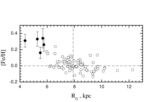
Figure 1: The radial distribution of the iron abundance. $Open\leavevmode\nobreak\ circles$ - data from Paper I, $black\leavevmode\nobreak\ circles$ - present results. 2-$\sigma$ interval is indicated for the stars from present study.

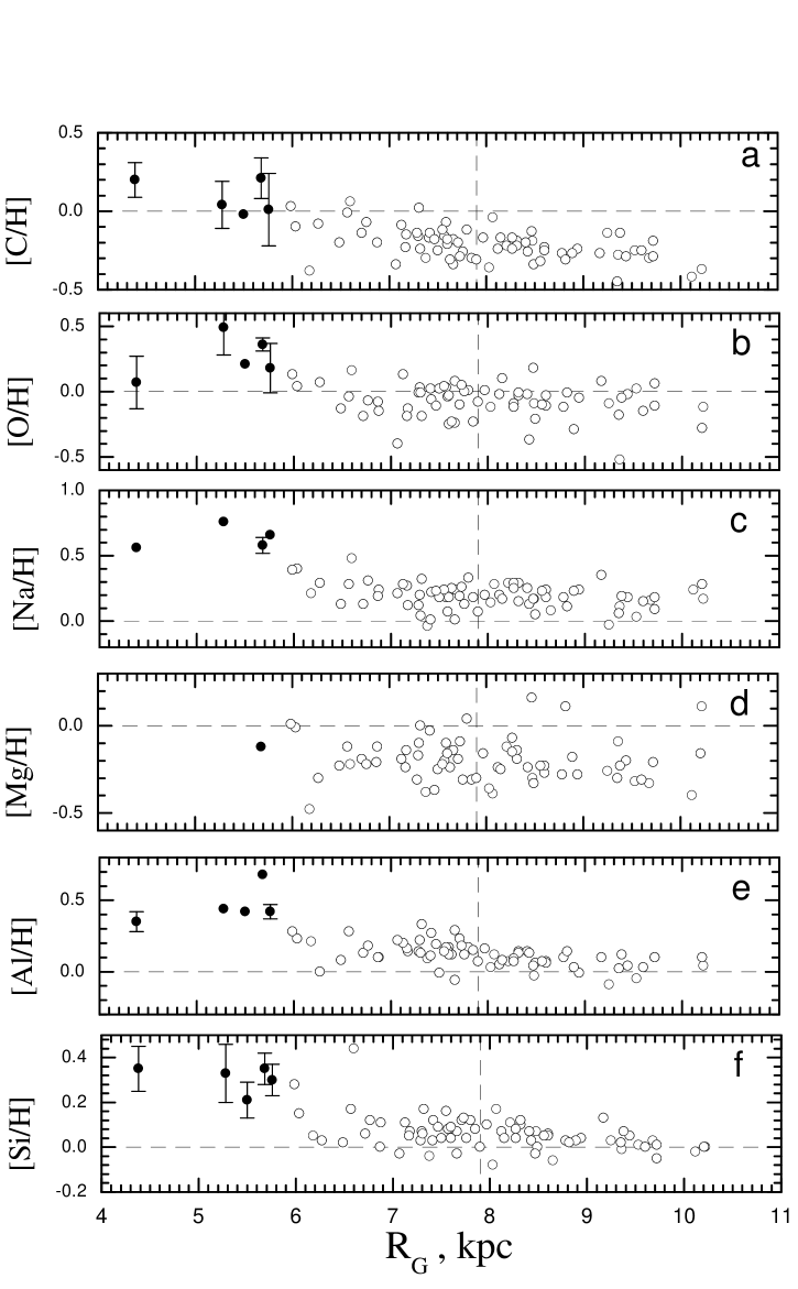
Figure 2: Same as Fig. 1, but for elements C–Si

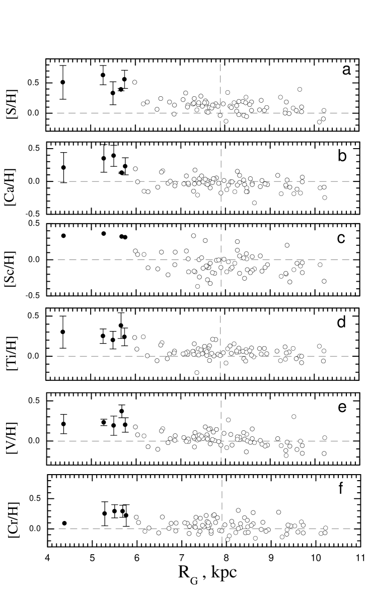
Figure 3: Same as Fig. 1, but for elements S–Cr

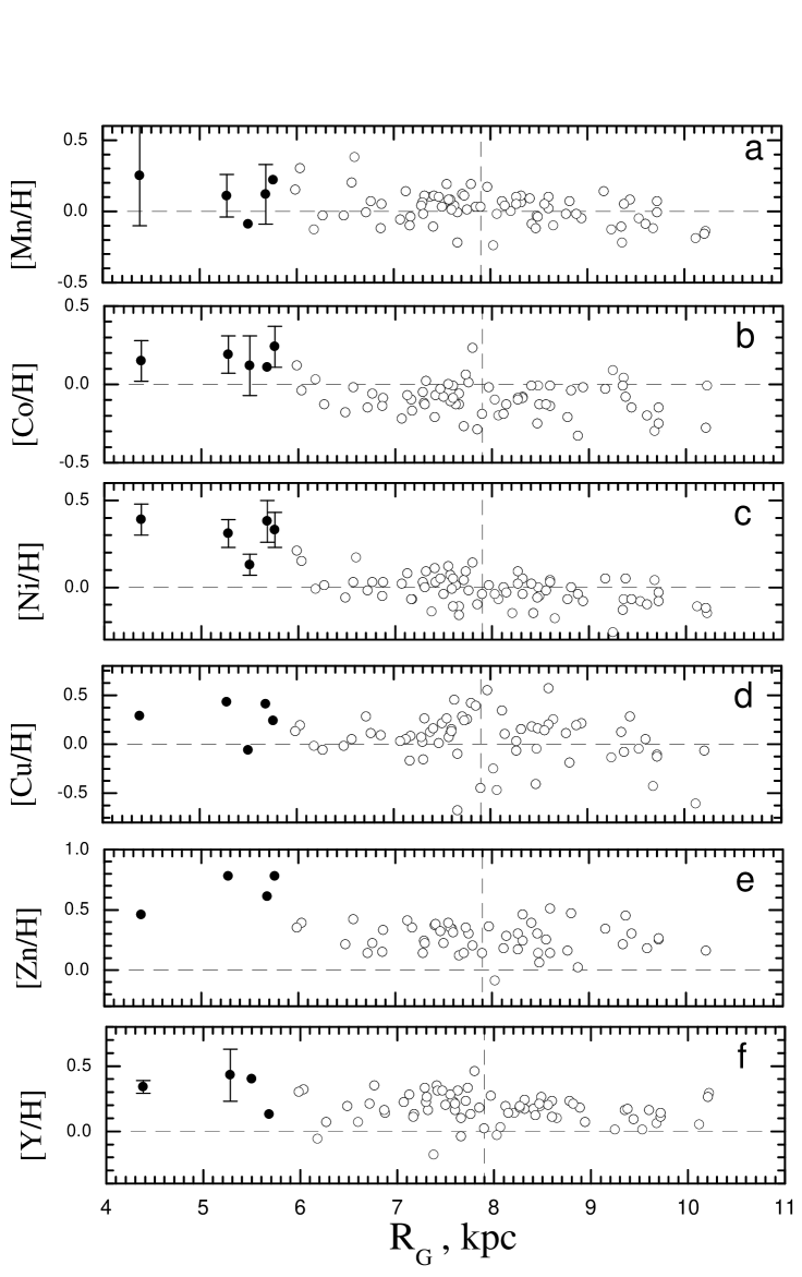
Figure 4: Same as Fig. 1, but for elements Mn–Y

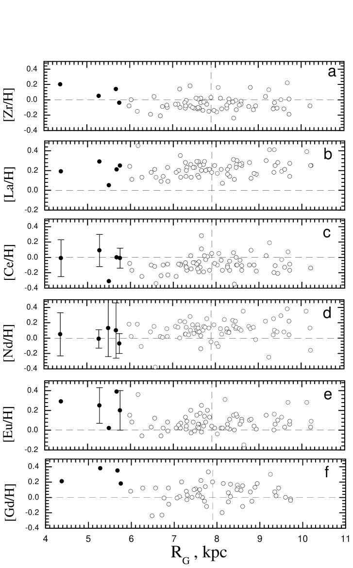
Figure 5: Same as Fig. 1, but for elements Zr–Gd

Below we briefly discuss a comparison between the metallicity distribution in the inner and middle part of galactic disc obtained from Cepheids with the most recent observational and theoretical results.

Recent determinations of the [Fe/H] gradient in the galactic disc have been on the basis of open cluster stars (see Friel 1995, 1999, Phelps 2000). Although these objects may have a wider age span than Cepheids, it is interesting to compare those gradients with our results, especially in view of the supposition that abundance gradients have not varied significantly in the last few Gyrs (Maciel & Quireza 1999, Maciel & Costa 2002). The review by Friel (1995) indicates a gradient of $-0.091$ dex kpc^-1, while a more recent presentation of data by the same group indicates a flatter value of $-0.06$ dex kpc^-1 (Friel 1999, Phelps 2000). Gradients similar to the steeper value above were also suggested by Carraro, Ng, Portinari (1998) and Bragaglia et al. (2000), and the results reported by Twarog, Ashman & Antony-Twarog (1997) also show some slope variation at about 10 kpc from the galactic center.

It can be seen that the above gradient results are intermediate between our steeper ”inner” gradient and the flatter ”outer” gradient shown in Fig. 6. In fact, if we roughly take an average of both regions we get d[Fe/H]/dR around $-0.08$ dex kpc^-1, which is close to the average gradient value for open clusters.

In Paper I we discussed the connection between the character of the elemental distribution in the solar neigbourhood and galactic bar which may induce the radial flows in the disc, and thus may produce a significant homogenization. Another observable phenomenon, which should be also caused by the bar, is a metallicity increase in the inner part of the disc. As was shown by Martinet & Fridli (1997), a rather young and strong bar produces two distinct gradients in the disc, one steep in the inner part, and another shallow in the outer region.

According to the model of Portinari & Chiosi (pch00 (2000)), a rotating bar sweeps the gas out from its co-rotation radius to the outer Lindblad resonance (located at approximately 5 kpc from the center), so that some local increase in the metallicity is expected in this region (see Fig. 14 for oxygen distribution from above mentioned paper). Qualitatively, this is confirmed by our observational results, but the detected oxygen overabundance at 4–6 kpc is higher than that predicted by the model. It should be noted that Portinari & Chiosi (pch00 (2000)) presumed in their model that bar has negligible influence on the disc beyond the outer Linblad resonance. They also used in the numerical simulation the velocity of the gas flows of about 0.1-1.0 km s^-1, although according to Stark (1984) and Stark & Brand (1989) the radial flows in the solar neighbourhood have a velocity of about 4 km s^-1.

Chiappini, Matteucci & Romano (cmr01 (2001)) presented a chemical evolution model assuming two accretion episodes in the Galaxy formation, but no radial flows. We overlay their ”model A” gradient on our data in Fig. 6. In the region from 4–6 kpc their model fits the data adequately but outward of 6 kpc the model predicts abundances significantly in excess of our observed values. If one rescales their gradient to [Fe/H] = 0 at the solar radius, then the predicted abundances in the inner region are significantly lower than the observed values. Note that as their model does not consider the possibility of homogenization in the disc from the radial flows triggered by a galactic bar, this factor might be responsible for some vertical shift between our observational data and the model prediction for the solar vicinity.

Summarizing, both an accretion-based galactic evolution model without the radial flows, and a model including the radial flows in the disc, produce a local increase of the abundance distribution at galactocentric distances of about 4–6 kpc. Such an increase was also detected in our observational study. Nevertheless, disagreement exists in the absolute abundances predicted by the models and those found from our observations. This disagreements may arise either from ignoring the radial flows, or from inadequate characteristics of the flows adopted in the model.

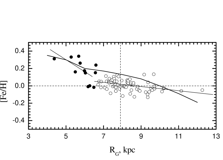
Figure 6: The radial distribution of the iron abundance for two zones. $Open\leavevmode\nobreak\ circles$ and $black\leavevmode\nobreak\ circles$ represent the Cepheids separated at 6.6 kpc. Theoretical prediction of ”inside-out” model A (Chiappini, Matteucci & Romano (cmr01 (2001)) - $thick\leavevmode\nobreak\ line$.

6 Conclusion

We supplemented our previous data on elemental abundance distributions in the solar neighborhood (Paper I) with new determinations based on Cepheids at distances of 4-6 kpc. Our new results together with previous gradient determinations (Paper I) show that the abundance distribution over the galactocentric distances 4–11 kpc cannot by represented by a single gradient value. More likely, the distribution is bimodal: it is flatter in the solar neighborhood with a small gradient, and becomes steeper towards the galactic center. The steepening begins at the distance about 6.5 kpc.

- (1) Andrievsky S.M., Kovtyukh V.V., Luck R.E., Barbuy B., Lépine J.R.D., Bersier D., Maciel W.J., Klochkova V.G., Panchuk V.E., Karpischek R.U., 2002, A&A 381, 32
- (2) Bragaglia A., Tosi M., Marconi G., Carretta E., 2000, Chemical evolution of the Milky Way, Eds. F. Matteucci, F. Giovannelli, Kluwer, 281
- (3) Carr J.S., Sellgren K., Balachandran S.C., 2000, ApJ 530, 307
- (4) Carraro G., Ng Y.K., Portinari L., 1998, MNRAS 296, 1045
- (5) Chiappini C., Matteucci F., Romano D., 2001, ApJ 554, 1044
- (6) Fernie J.D., Evans N.R., Beattie B., Seager S., 1995, IBVS 4148, 1
- (7) Friel E.D., 1995, ARA&A 33, 381
- (8) Friel E.D., 1999, Ap&SS 265, 271
- (9) Galazutdinov G.A., 1992, SAO RAS Prepr. No.92
- (10) Maciel W.J., Quireza C., 1999, A&A 345, 629
- (11) Maciel W.J., Costa, R.D.D., 2002, IAU Symp. 209, in press
- (12) Martinet L., Friedli D., 1997, A&A 323, 363
- (13) Phelps R., 2000, Chemical evolution of the Milky Way, Eds. F. Matteucci, F. Giovannelli, Kluwer, 239
- (14) Portinari L., Chiosi C., 2000, A&A 355, 929
- (15) Ramírez S.V., Sellgren K., Carr J.S., Balachandran S.C., Blum R., 2000, ApJ 537, 205
- (16) Stark A.A., 1984, ApJ 281, 624
- (17) Stark A.A., Brand J., 1989, ApJ 339, 763
- (18) Twarog B.A., Ashman K.M., Antony-Twarog B.J., 1997, AJ 114, 2556