Effects of the magnetic fields on the helium white dwarfs structure.

Abstract

In this paper the effect of the magnetic field on the form of the equation of state and helium white dwarfs structure are discussed. The influence of the temperature and magnetic field on white dwarfs parameters have been investigated. The mass-radius relations for different parameters were obtained. The occurrence of unstable branches in the mass-radius relation are presented for the temperature equals $T=3$ $10^{8}$ $K$ and for different values of the strength of magnetic field. Theoretical model of the star with two Landau levels is obtained.

Department of Astrophysics and Cosmology, Institute of Physics, University of Silesia, Uniwersytecka 4, 40-007 Katowice, Poland.

PACS numbers 64, 65, 97

1 Introduction

Properties of matter in strong magnetic field has been the subject of investigations in astrophysics of white dwarfs and neutron stars. It is motivated by the fact that magnetic fields of the order of $10^{8}$ $Tesla$ - $10^{9}$ $Tesla$ are known to exist in many cases of white dwarfs and neutron stars. White dwarfs are compact objects with masses comparable to that of the Sun, radii of the order of several thousands of kilometers and mean densities about $10^{9}$ $kg$ $m^{-3}$. These stars no longer burn nuclear fuel. They are slowly cooling as they radiate away their residual thermal energy. White dwarfs radii decrease with increasing mass. In accordance with theoretical predictions there is a critical value of white dwarf mass known as $Chadrasekhar$ $mass$ which is predicted to be

$$M_{Ch}=5.8\ Y_{e}^{2}\ M_{\odot}$$

where $Y_{e}$ is the fraction of electrons. This is the pressure of degenerate electrons which supported the star against collapse. The electrons are supposed to be degenerate with arbitrary degree of relativity (in this paper the unit in which $c=\hbar=1$ was used) $x=k_{F}/m_{e}$ and it various with the density. Helium ions provide the mass of the star and their contribution to the pressure is negligible [1, 2, 3].
The ions form a regular lattice which minimizes the energy. Detailed models of white dwarfs were given by Salpeter (1967) who derived conditions for their solidification and determined properties of the lattice.
A number of white dwarfs with strong magnetic fields was discovered (Kemp et al. 1970; Putney 1995; Reimers et al. 1996) [4, 5, 6] and extensively studied (Jordan 1992; Chanmugan 1992)[7, 8].
In about 3-4 $\%$ of all white dwarfs magnetic fields have been detected ranging from $2$ $10^{-1}$ $Tesla$ up to $10^{5}$ $Tesla$. The magnetic white dwarfs where a surface magnetic field on the order of $10$ $Tesla$ $\sim$ $10^{5}$ $Tesla$ and an interior field of $10^{5}$ $Tesla$ $\sim$ $10^{9}$ $Tesla$ are estimated. The magnetic field may causes considerable effects on the structure of white dwarfs. Earlier work of Ostriker and Hartwick (1968) and recent calculations of Such and Mathews (2000) predicted an increase of white dwarf radii in the presence of internal magnetic fields [9, 10]. In this paper the influence of the temperature and magnetic field on white dwarfs parameters have been investigated. The mass-radius relations for different parameters were obtained.
This paper is organized as follows.
In Sect.1 are presented the general properties of white dwarfs. In Sect.2 the employed equation of state (EOS) is obtained in magnetic fields model with different temperatures. Finally the EOS is used to determine the equilibrium configurations of white dwarfs. The interesting fact is the existence of unstable branches on the mass-radius relation for temperature $T=3$ $10^{8}$ $K$ and different values of the strength of magnetic field, which indicate that there are several possible evolutionary tracks. Finally, in Sect.3 the main implications of the results are discussed.

2 The white dwarfs in the magnetic fields model

This paper presents the model of helium white dwarf in which the main contribution to the pressure comes from ultra-relativistic electrons. Corrections from finite temperature and magnetic field are also included. Having made the assumption that the ionised uniform helium plasma forms the interior of such an object one can say that the white dwarf matter consists of electrically neutral plasma which comprises charged ions $(^{4}He)$ and electrons.
The Lagrangian density function in this model can be represented as the sum

$${\mathcal{L}}={\mathcal{L}_{e}}+{\mathcal{L}_{G}}+{\mathcal{L}_{ion}}+{\mathcal{L}_{QED}},$$ (1)

where ${\mathcal{L}_{e}}$, ${\mathcal{L}_{G}}$ describe the electron and gravitational terms, respectively. The ${\mathcal{L}_{ion}}$ determines the ionized helium and ${\mathcal{L}_{QED}}$ is the Lagrangian density function of the QED theory.
The electron part of the Lagrangian is given by

$${\mathcal{L}_{e}}=i\overline{\psi_{e}}\gamma^{\mu}D_{\mu}\psi_{e}-m_{e}\overline{\psi_{e}}\psi_{e},$$

where $D_{\mu}$ is the covariant derivative defining as$\,\,D_{\mu}=\partial_{\mu}-ieA_{\mu}\,$ and $e$ is the electron charge. The Dirac equation for electrons obtained from the Lagrangian function ${\mathcal{L}}$ has the form

$$(i\gamma^{\mu}D_{\mu}-m_{e})\psi_{e}=0.$$

The vector potential is defined as $A_{\mu}=\{A_{0}=0,\,A_{i}\}$ where

$$A_{i}=-\frac{1}{2}\varepsilon_{ilm}x^{l}B_{0}^{m}.$$

The gauge in which uniform magnetic field B lies along the z-axis was chosen

$$B_{0}^{m}=(0,0,B_{z}).$$

The magnetization is given by the contribution of the electrons and depends on the density of particles and antiparticles. Different from zero magnetization generates internal molecular field $B_{z}=\mu\mathcal{M}_{z}\neq 0$. The energy-momentum tensor can be calculated taking the quantum statistical average

$$\bar{T}_{\mu\nu}=<T_{\mu\nu}>,$$

where

$$T_{\mu\nu}=2\frac{\partial{{\mathcal{L}}}}{\partial g^{\mu\nu}}-g_{\mu\nu}{\mathcal{L}}.$$

In general in the presence of finite magnetization the pressure is anisotropic. For the electrically charge particles, different equations of state for directions paraller and perpendicular to the magnetic field can be obtained. Thus the energy-momentum tensor has the form

$$<T_{\mu\nu}>=\left(\begin{array}[]{cccc}\varepsilon=\rho&0&0&0\\ 0&P&0&0\\ 0&0&P&0\\ 0&0&0&P+\mu\mathcal{M}_{z}B_{z}\end{array}\right).$$ (2)

This anisotropy in the pressure leads to a magnetostriction effect in the quantum magnetized gas of charged particles. In the classical case nonzero magnetization produces a flattening effect in white dwarfs and neutron stars models [11] similarly like in the case of rotating stars [12] . Einstein equations (in isotropic case) leads to the standard Tolman-Oppenheimer-Volkov equations [13]. The equations describing masses and radii of white dwarfs are determined by the proper form of the equation of state. The aim of this paper is to calculate the equation of state for helium white dwarfs with the assumptions of finite temperature and in the presence of magnetic field.
The properties of an electron in external magnetic field have been studied, for example by Landau and Lifshitz in 1938 [14]. In this paper the effects of high magnetic field on the equation of state of a relativistic, degenerate electron gas is considered. The motion of free electrons in homogeneous magnetic field of the strength $B$ perpendicular to the field is confined by the oscillatory force determined by the field $B$ and is quantized into Landau levels with the energy $nB$, $n=0,1,\ldots$. In the case of nonrelativistic electrons the energy spectrum is given by the relation

$$E_{n,p_{z}}=n\omega_{c}+\frac{p_{z}^{2}}{2m_{e}}$$

where $n=j+\frac{1}{2}+s_{z}$, the cyclotron energy $\omega_{c}=eB/m_{e}$, $p_{z}$ is the momentum along the magnetic field and can be treated as continuous. For extremly high magnetic field the cyclotron energy is comparably with the electron rest mass energy and this is the case when electrons became relativistic. Introducing the idea of the critical magnetic field strength $B_{c}=m_{e}^{2}/\mid e\mid$ which equals $4.414\times 10^{9}$ $Tesla$, it is easy to distinguish between nonrelativistic and relativistic cases, for $B\geq B_{c}$ the relativistic Dirac equation for electrons have to be used. The obtained dispersion relation now takes the form

$$E_{n,p_{z}}=\sqrt{p_{z}^{2}+m_{e}^{2}+2eB_{z}n}.$$ (3)

Along the field the motion is free, quasi one-dimensional with the modified density of states. The electron density of states in the absence of the magnetic field is replaced by the sum

$$2\int\frac{d^{3}{p}}{(2\pi)^{3}}\rightarrow 2\Sigma_{n=0}^{\infty}[2-\delta_{n0}]\int\frac{eB_{z}}{(2\pi)^{2}}dp_{z},$$

where the symbol $\delta_{n0}$ denotes the Kronecker delta [10] and thus the spin degeneracy equals 1 for the ground ($n=0$) Landau level and 2 for $n\geq 1$. The redefined density of states makes the distinctive difference between the magnetic and non-magnetic cases. The equation (3) implies that for $n=0$, $E_{0}=\sqrt{p_{z}^{2}+m_{e}^{2}}$ whereas for $n\geq 1$ $E_{n}=\sqrt{p_{z}^{2}+m_{e}^{\star 2}}$. These relations indicate that the quantity $m_{e}^{\star}$ defined as $m_{e}^{\star 2}=m_{e}^{2}+2eB_{z}n$ depends on the presence of the magnetic field and can be interpreted as an effective electron mass which is different from electron mass for $n\geq 1$. The number density of electrons at zero temperature is given by

$$n_{e}=\Sigma_{n=0}^{n=n_{max}}[2-\delta_{n0}]eB2p_{e}^{F}.$$

The maximum Landau level is calculated from the condition $(p_{e}^{F})^{2}\geq 0$. One can define the critical magnetic density $\rho_{B}$, which denotes the limiting density

$$\rho_{B}=0.802\ Y_{e}^{-1}\gamma^{3/2}g\ cm^{-3},$$ (4)

for densities lower than $\rho_{B}$ only the ground Landau level is present.
Thermodynamic properties of a free electron gas in the magnetic fields at finite temperature have to be investigated. The temperature affects the electron motion in external magnetic fields. Finite temperature and decreasing value of the strength of magnetic field tend to smear out Landau levels. The number density of electrons in the presence of a magnetic field can be expressed now as

$$n_{e}=\frac{2m_{e}^{3}\gamma}{4\pi^{2}}\Sigma_{n=0}^{\infty}[2-\delta_{n0}](I_{0,0,+}(z/t,1+2\gamma n)-I_{0,0,-}(z/t,1+2\gamma n))$$ (5)

where the Fermi integral

$$I_{\lambda,\eta\pm}(u,\alpha)=\int\frac{(\alpha+x^{2})^{\lambda/2}x^{\eta}dx}{e^{\left(\sqrt{\alpha+x^{2}}\mp u\right)}+1}$$ (6)

was used [15, 16], $z=\mu_{0}/m_{e}$, $t=k_{B}T_{0}/m_{e}$, $u=z/t$ and $\gamma=B_{z}/B_{c}$. Similarly to Fermi temperature which is given by

$$T_{F}=E_{F}/k_{B}=(m_{e}/k_{B})\epsilon_{F}\qquad(\mathrm{for}\leavevmode\nobreak\ \leavevmode\nobreak\ \rho<\rho_{B}),$$ (7)

one can define a magnetic temperature

$$T_{B}={\frac{\Delta E_{B}}{k_{B}}}={\frac{m_{e}}{k_{B}}}\left(\sqrt{1+2n_{\mathrm{max}}\gamma+2\gamma}-\sqrt{1+2n_{\mathrm{max}}\gamma}\right)$$ (8)

where $\Delta E_{B}$ is the energy difference between the $n_{L}=n_{\mathrm{max}}$ level and the $n_{L}=n_{\mathrm{max}}+1$ level. For $\rho=\rho_{B}$ these temperatures equal $T_{F}=T_{B}$. Knowing the value of magnetic temperature $T_{B}$ one can describe how the properties of free electron gas changes at finite temperature and the presence of magnetic field. The influence of magnetic field is most significant for $\rho\leq\rho_{B}$ and $T\leq T_{B}$ when electrons occupy the ground Landau level. In this case one can deal with the strong quantizing gas and magnetic field modifies all parameters of the electron gas. For example, for degenerate, nonrelativistic electrons the pressure is proportional to $\rho^{3}$ and this form of the equation of state one can compare with that for the case B=0 for which $P\sim\rho^{5/3}$. When $\rho>\rho_{B}$ the Fermi temperature is still greater than magnetic temperature $T_{B}$ electrons are degenerate and there are many Landau levels, now the level spacing exceeds $k_{B}T$. The properties of the electron gas are only slightly affected by magnetic field. With increasing temperature, there is the thermal broadening of Landau levels, when $T\geq T_{B}$, the free field results are recovered. For $T\gg T_{B}$ there are many Landau levels and the thermal widths of the Landau levels are higher than the level spacing. The magnetic field does not affects the thermodynamic properties of the gas [16].

The total pressure of the system can be described as the sum of the pressure coming from electrons and ions plus small corrections coming from electromagnetic field

$$P=P_{e}+P_{ion}+P_{QED}.$$

The contributions from the same constituents form the energy density

$$\varepsilon=\varepsilon_{e}+\varepsilon_{ion}+\varepsilon_{QED}.$$

The electron pressure and energy density are defined with the use of Fermi integral

$$P_{e}=\frac{2\gamma m_{e}^{4}}{4\pi^{2}}\Sigma_{n=0}^{\infty}[2-\delta_{n0}](I_{-1,2,+}(z/t,1+2\gamma n)+I_{-1,2,-}(z/t,1+2\gamma n))$$ (9)

$$\varepsilon_{e}=\frac{2\gamma m_{e}^{4}}{4\pi^{2}}\Sigma_{n=0}^{\infty}[2-\delta_{n0}](I_{1,0,+}(z/t,1+2\gamma n)+I_{1,0,-}(z/t,1+2\gamma n)).$$ (10)

The ions are very heavy and treated as classical gas. The influence of magnetic field for ions is very small so we have neglected this correction. The pressure and energy density dependence on the chemical potential $\mu_{0}\,\,$ determines the form of the equation of state, which is calculated in the flat Minkowski space-time. The obtained form of the equation of state is the base for calculating macroscopic properties of the star. In order to construct the mass-radius relation for given form of the equation of state the OTV equations have to be solved

$$\frac{dP(r)}{dr}=-\frac{G}{r^{2}}(\rho(r)+P(r))\frac{(m(r)+4\pi P(r)r^{3})}{(1-\frac{2Gm(r)}{r})}$$ (11)

$$\frac{dm(r)}{dr}=4\pi r^{2}\rho(r).$$ (12)

However, presence of strong gravitational field of the star causes the dependence of the temperature and chemical potential on the gravitational potential. In this paper together with the calculated form of the equation of state for completely ionised pure helium plasma the chosen values of central density $\rho_{c}$ changes from $10^{7}$ $kg$ $m^{-3}$ to $10^{14}$ $kg$ $m^{-3}$. For such parameters the value of magnetic field and temperature were limited to the following ranges $T(0-10^{9})$ $K$, $\gamma(0-1)$, respectively. Having solved OTV equations the pressure $P(r)$, mass $m(r)$ and density $\rho(r)$ were constructed. To obtain the total radius $R$ of the star the fulfillment of the condition $P(r)=0$ is necessary. The results are presented in figures 1-10. Studying the properties of the star in the framework of the general-relativistic Thomas-Fermi model one can made the assumption that the temperature and chemical potential are metric dependent local quantities and the gravitational potential instead of Poisson’s equation satisfies Einstain’s field equations. The metric is static, spherically symmetric and asymptotically flat

$$g_{\mu\nu}=\left(\begin{array}[]{cccc}e^{\nu}&0&0&0\\ 0&-e^{\lambda}&0&0\\ 0&0&-r^{2}&0\\ 0&0&0&-r^{2}sin^{2}\theta\end{array}\right).$$ (13)

Its coefficients can be determined from Einstain equations and written as follows

$$e^{-\lambda}=1-\frac{2Gm(r)}{r}.$$

The energy-momentum conservation

$$T_{;\nu}^{\mu\nu}=0$$

which for spherically symmetric metric (13) can be written as

$$\frac{d\nu}{dr}=-\frac{2}{P+\rho}\frac{dP}{dr}$$ (14)

together with the Gibbs-Duhem relation and with the assumption that the heat flow and diffusion vanishes [17] give the condition

$$\frac{\mu}{T}=\mathrm{const}.$$ (15)

This implies that the temperature and chemical potential be come local metric functions

$$T(r) = e^{-\nu(r)/2}T_{0}$$ (16)

$$\mu(r) = e^{-\nu(r)/2}\mu_{0}$$ (17)

where $T_{0}$ and $\mu_{0}$ are constants equal to the temperature and chemical potential at infinity. The temperature $T_{0}$ may be chosen arbitrarily as the temperature of the heat-bath. First equation in (16) is the well known Tolman condition for thermal equilibrium in a gravitational field [18]. For given values $\mu_{0}$ and $T_{0}$ one can obtain self-consistency equations defining general-relativistic Thomas-Fermi equation. Now, the Fermi-Dirac distributions are defined as [19]

$$\frac{1}{e^{\left(\sqrt{1+x^{2}+2\gamma n}-z_{0}\right)/t_{0}}+1}\rightarrow\frac{1}{e^{\left(e^{\nu(r)/2}\sqrt{1+x^{2}+2\gamma n}-z_{0}\right)/t_{0}}+1}$$

$$=\frac{1}{e^{\left(\sqrt{1+x^{2}+2\gamma n}-z(r)\right)/t(r)}+1}.$$

In the result instead of the OTV equilibrium equations together with the equation of state which was calculated in the flat space-time one can derived three self-consistency equations (11,12,14) together with local form of the equation of state being now the function of $r$. This is of particular importance in the case of the strong gravitational fields.

3 Discussion

In order to construct the mass-radius relation for white dwarfs the proper form of the equation of state have to be enumerated. For our needs we have chosen the pure helium plasma as the main constituent of the white dwarf interior. All calculations were performed at finite temperature and different from zero magnetic field and compared with those of zero temperature and without magnetic field. In Figure 1 the applied form of the equation of state for magnetic and non-magnetic white dwarfs were presented. The zero temperature case is compared with the one obtained for temperature $6\times 10^{8}$ $K$. For temperature equals zero there are clearly visible Landau levels which are smeared out when the temperature is different from zero and the strength of magnetic field is decreased. The density profile for helium magnetic and non-magnetic white dwarfs for different values of temperatures and central density $\rho_{c}$ equals $10^{10}$ $kg$ $m^{-3}$ was shown in Figure 2. As in the case of the EOS one can distinguish Landau levels for zero temperature case. The Fermi temperature for non-magnetic white dwarfs with the fixed value of the central density $\rho_{c}=10^{10}$ $kg$ $m^{-3}$ is calculated and equals $T_{F}=1.023\times 10^{10}$ $K$. The estimated value of the magnetic field temperature for white dwarfs with the strength of magnetic field $\gamma=1$ $(\rho_{c}=10^{10}\ kg\ m^{-3})$ is $T_{B}=1.27\times 10^{9}$ $K$. Theoretical model of helium white dwarf with different electron masses which correspond to the ground Landau level $(n=0)$ and the one for $n=1$ is presented in Figure 2. The change of mass can be interpreted as the appearance two shells with distinctively different value of densities. For the presented form of the EOS the mass-radius relations were constructed. These relations are presented in Figure 3. Of special interest is the case when the temperature equals $10^{8}$ $K$ because the appearance of unstable areas. The same is visible on the relation mass-central density (Figure 4). There are marked points $A$, $B$, $C$ on mass-radius and mass-central density relations. These points represents the stable configurations ($A$ and $C$) whereas point $B$ refers to the unstable one. Figures 5 and 6 present sequences on the mass-radius relations for fixed value of temperature. In Figure 5 the chosen value of the temperature equals $T=6\times 10^{8}$ $K$ whereas in Figure 6 the temperature equals $T=3\times 10^{8}$ $K$ . In both figures the strength of magnetic field changes from $\gamma=0$ to $\gamma=1$. For comparison the zero temperature mass-radius relation obtained was presented. For increasing value of the magnetic field white dwarfs increase their mass. However, the asymptotic value of $Chadrasekhar$ $mass$ is not exceeded. In the range of low densities together with increasing value of the temperature the radii of these objects decrease. The mass-central density relations for helium white dwarfs are presented in Figures 7 and 8. Thick full curves stable branches, whereas thin full curves depict the unstable branches (Figure 8). The minimum and maximum of helium white dwarf star masses are represented by the extrema of $M$. These are point where the stable and dynamically unstable branches merge. Stable branches are those with $\frac{dM}{d\rho_{c}}>0$. The existence of unstable branches enables different evolution tracks. The temperature profile is presented in the Figure 9 for the fixed value of the central density $\rho_{c}$. The temperature is changed slightly with the radius in agreement with the value of gravitational potential which is much smaller in comparison with neutron stars. White dwarfs with known values of masses and radii which collected in Table 1 are marked on the obtained mass-radius relations in Figure 10. In Figure 10 the theoretical point $m$ is marked. It represents the model of a star formed with one-dimensional electron gas. The changes of electron mass depend on the value of the Landau level $n$. The constructed configuration has distinctive shells with different values of the electron mass which is directly connected with the population of Landau levels. For $n=0$ (only the ground Landau level is populated) the electron mass is unchanged whereas for $n=1$, one can deal with the modified by the magnetic field electron mass.

4 Figure captions.

Figure 1
The equation of state for different temperature and strength of magnetic field cases.
Figure 2
The density profile for helium magnetic white dwarf and for non-magnetic white dwarf for different temperatures and $\rho_{c}=10^{10}$ $kg/m^{-3}$.
Figure 3
The mass-radius relation for white dwarf with different temperature cases.
Figure 4
The mass $M$ dependence on the central density $\rho_{c}$ for different temperature values.
Figure 5
The mass-radius diagram for helium white dwarfs for temperature $T=6$ $10^{8}$ $K$ and the strength of magnetic field $\gamma=0.1-1$. The solid line denotes the mass-radius relation for $T=0K$.
Figure 6
The mass-radius diagram for helium white dwarfs for temperature $T=3$ $10^{8}$ $K$ and the strength of magnetic field $\gamma=0.1-1$.
Figure 7
The mass $M$ dependence on the central density $\rho_{c}$ for temperatures $T=0K$ and $T=6$ $10^{8}$ $K$.
Figure 8
The mass $M$ dependence on the central density $\rho_{c}$ for temperatures $T=0K$ and $T=3$ $10^{8}$ $K$.
Figure 9
The temperature profile for different central density.

Figure 10
The mass-radius relation for white dwarf with different values of temperature with marked observational white dwarfs. The point $m$ denotes the theoretical model of the star with Landau levels $n_{L}=0$, $n_{L}=1$ which are clearly visible in the Figure 2. The mass and radius for this configuration is calculated $R=0.92$ $(100R/R_{\odot})$, $M=1.18$ $M_{\odot}$.

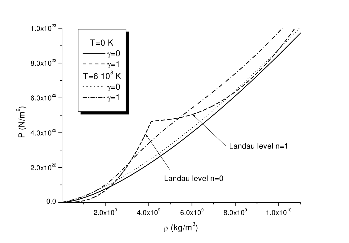
Figure 1:

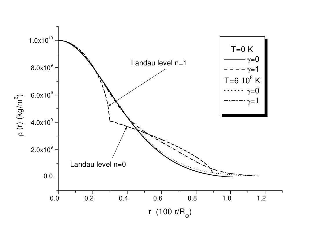
Figure 2:

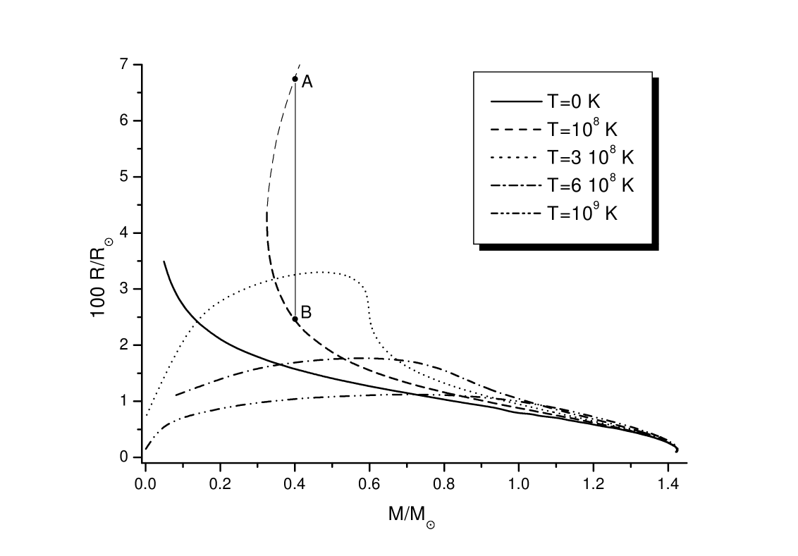
Figure 3:

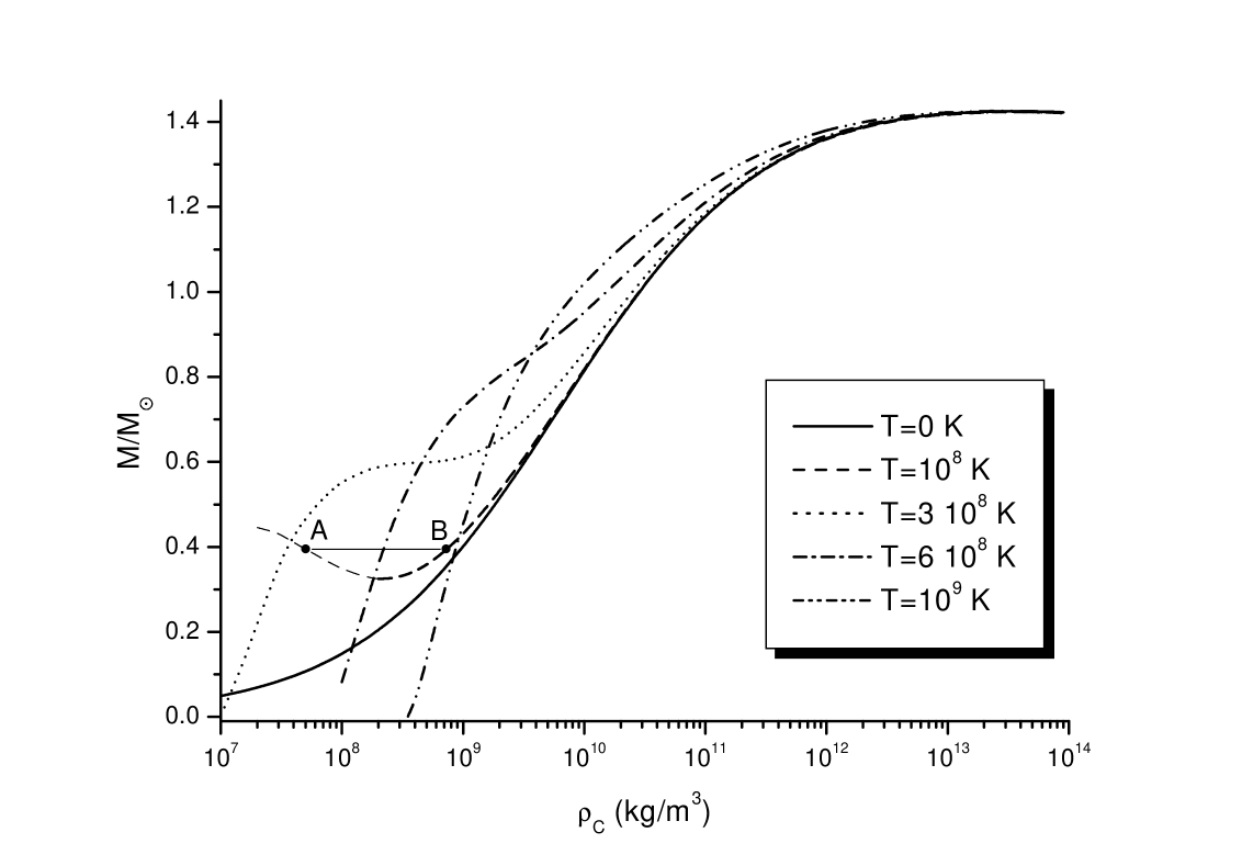
Figure 4:

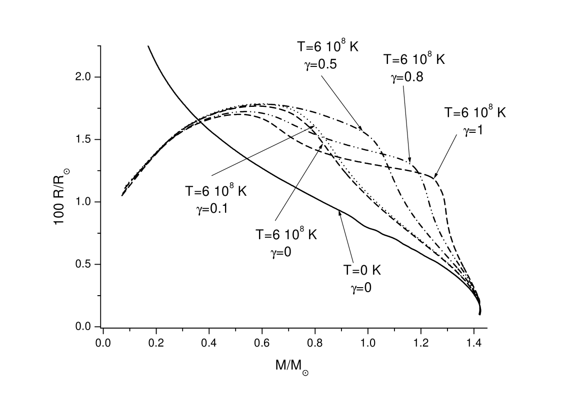
Figure 5:

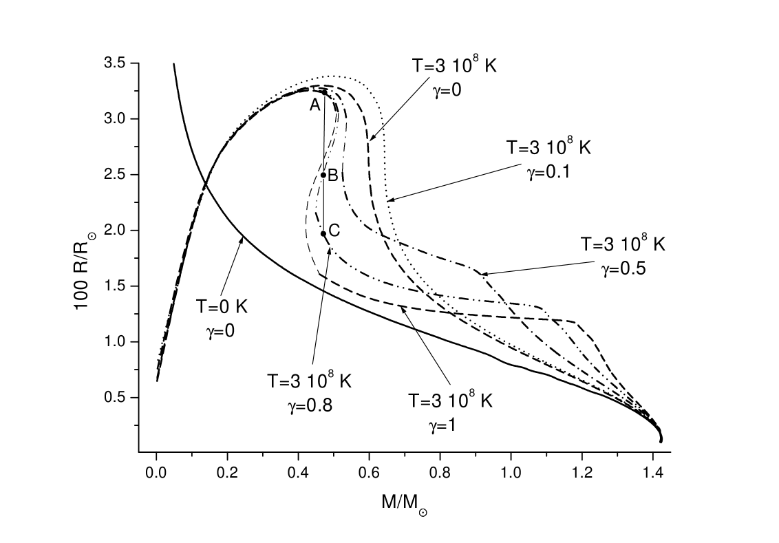
Figure 6:

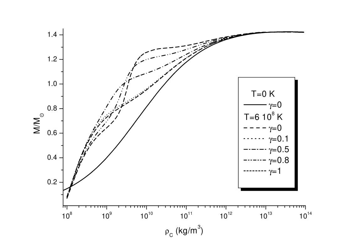
Figure 7:

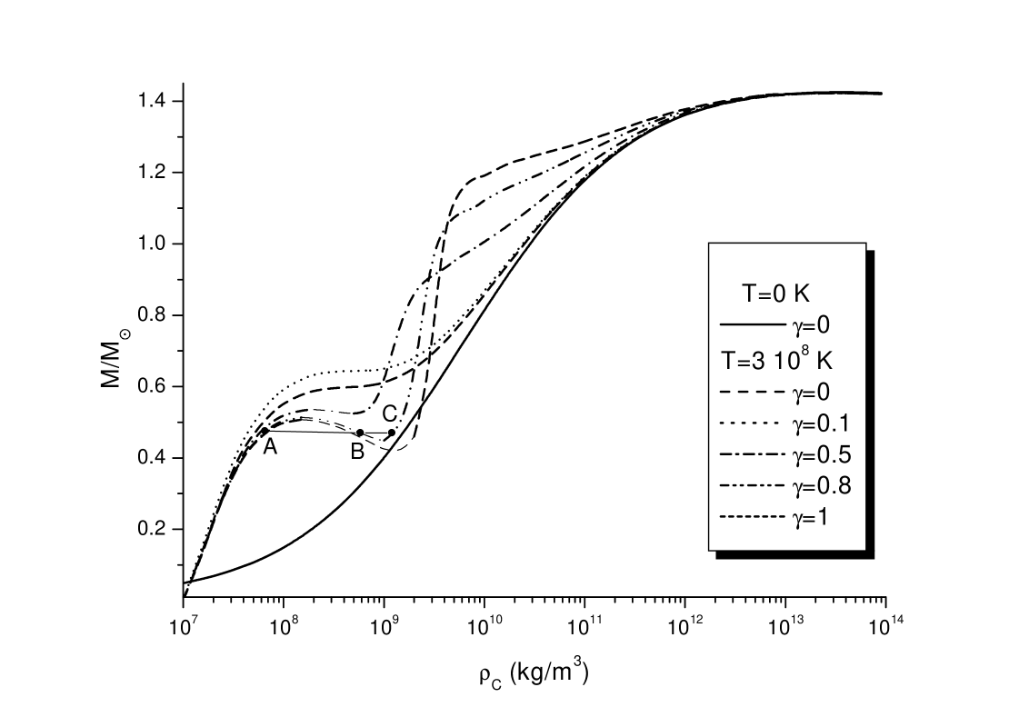
Figure 8:

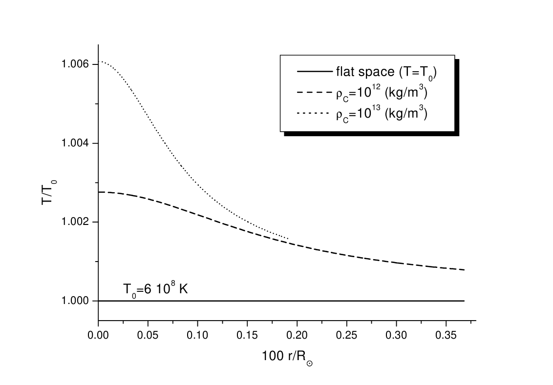
Figure 9:

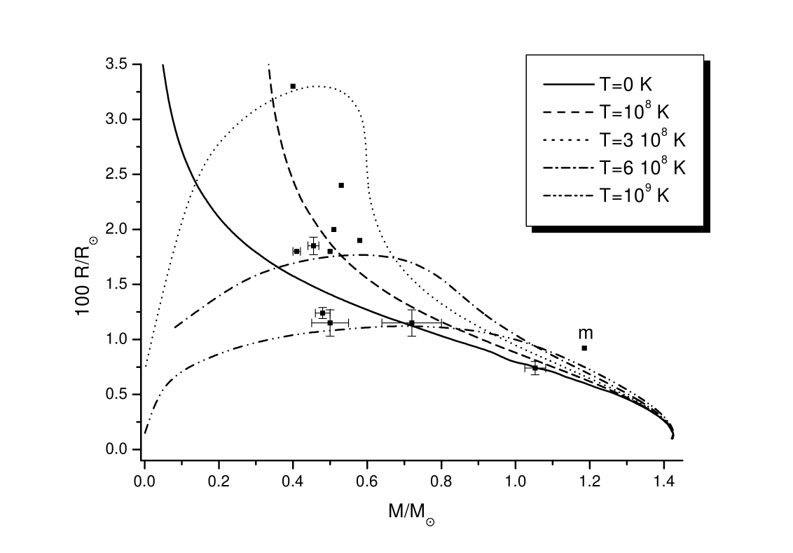
Figure 10:

$Object$	$M\,[\,M_{\odot}\,]$	$R\,[\,\frac{100R}{R_{\odot}}\,]$	$Ref.$
$Syriusz$B	$1.053\pm 0.028$	$0.74\pm 0.06$	[1]
40 Eri B	$0.48\pm 0.02$	$1.24\pm 0.05$	[1]
Stein 2051	$0.50\pm 0.05$ $or$ $0.72\pm 0.08$	$1.15\pm 0.12$	[1]
DA	$0.45\pm 0.015$	$1.85\pm 0.08$	[20]
GD448	$0.41\pm 0.01$	$1.8$	[21]
GD191-B2B	$0.51$	$2.0$	[22]
Feige	$0.50$	$1.8$	[22]
WD2218+706	$0.40$	$3.3$	[22]
REJ0558+165	$0.58$	$1.9$	[22]
REJ1738+665	$0.53$	$2.4$	[22]

Table 1: The masses and radii for some typical white dwarfs.

References

- [1] Shapiro S L and Teukolsky S A, 1983 Black hols, white dwarfs and neutron stars New Yor
- [2] Balberg S and Shapiro S L, The properties of matter in white dwarfs and neutron stars Preprint astro-ph/0004317
- [3] Glendenning N K, 2000, Compact stars. Nuclear Physics, Particle Physics, and General Relativity, Springer
- [4] Kemp J C, Swedlund J B, Landstreet J D, Angel J R P, 1970 ApJ L77 161
- [5] Putney A, 1995 ApJ L67 451
- [6] Reimers D, Jordan S, Koester D, Bade N, Köhler Th, Wisotzki L, 1996 A & A 311 572
- [7] Chanmugan G, 1992 ARA & A 30 143
- [8] Jordan S 1992 A & A 265 570
- [9] Ostriker J P, Hartwick F D A, 1968 ApJ 153 797
- [10] Suh In-Seang, Mathews G J, 2000 ApJ 530 949
- [11] Chaichian M, Masood S S, Montonen C, Martinez Perez A, Rojas Perez H, Quantum magnetic collapse Preprint hep-ph/9911218 v 2
- [12] Konno K, Obata T and Kojima Y, 1999, Deformation of relativistic magnetized stars, A & A 352 211-216
- [13] Mańka R, Zastawny-Kubica M, Brzezina A and Bednarek I, 2001 Protoneutron star in the relativistic mean-field theory J. Phys. G: Nucl. Part. Phys. 27 1917-1938
- [14] Landau L D, Lifshitz E M, 1938 Statistical Mechanics Claredon, Oxford
- [15] Bisnovatyi-Kagan G S, 2000, Stellar Physics Springer, Berlin
- [16] Lai D, Matter in strong magnetic fields Preprint astro-ph/0009333 v 2
- [17] Israel W,1976 Ann. Phys. 100 310
- [18] Tolman R C, 1934 Relativity Thermodynamics and Cosmology Clarendon, Oxford 312-317
- [19] Bilić N, Viollier R D, 1999 Gen.Rel.Grav. 31 1105-1113
- [20] Benedict G F, McArthur B E et al, Interferometric astrometry of the detected white dwarf-M dwarf binary Feige 24 using HST fine guidance sensor 3: white dwarf radius and component estimates Preprint astro-ph/0001387
- [21] Maxted P F L, Marsh T R et al, 2001 The mass-radius of the M dwarf companion to GD 448 Mon. Not. R. Astron. Soc. 000 1-8 (1999)
- [22] Bannister N P, Barstow M A et al, STIS observations of five hot DA white dwarfs Preprint astro-ph/0010313