Optical SETI: A Spectroscopic Search for Laser Emission
from Nearby Stars$~{}^{1}$

Abstract

We have searched for nonastrophysical emission lines in the optical spectra of 577 nearby F, G, K, and M main–sequence stars. Emission lines of astrophysical origin would also have been detected, such as from a time–variable chromosphere or infalling comets. We examined $\sim$20 spectra per star obtained during four years with the Keck/HIRES spectrometer at a resolution of 5 km s${}^{-1}~{}$, with a detection threshold 3% of the continuum flux level. We searched each spectrum from 4000 Å – 5000 Å  for emission lines having widths too narrow to be natural from the host star, as well as for lines broadened by astrophysical mechanisms. We would have detected lasers that emit a power, $P>$50 kW, for a typical beam width of $\sim$0.01 arcsec (diffraction–limit from a 10-m aperture) if directed toward Earth from the star. No lines consistent with laser emission were found.

1 Introduction

Most searches for signals from extraterrestrial intelligent civilizations (SETI) have concentrated on radio wavelengths (e.g. Tarter 2001, Cullers 2000, Werthimer et al. 2000, Leigh and Horowitz 2000). However, a preferred wavelength for SETI work has proved elusive. The motivation for this project stemmed from the suggestion of Schwartz and Townes (1961) that advanced civilizations might use optical or near–infrared lasers as an efficient means of interstellar communication (Townes 1998, Lampton 2000). The advantages of optical wavelengths over radio include the higher bandwidth and the narrower diffraction–limited beam size to promote private communication. In addition, the technology needed to produce lasers with detectable powers is not far from current Earth technology (§2.3).

Optical SETI (OSETI) projects are currently designed to detect highly energetic, pulsed lasers and continuous–wave lasers. Such efforts include dedicated searches, piggyback searches, and data mining. Many OSETI projects are designed to detect pulsed lasers using fast photometry (Howard et al. 2000, Bhathal 2000, Werthimer et al. 2001). Two or three photodetectors are employed to search for laser pulses having a duration of $\sim$1 ns in broadband visible light. A high–powered nanosecond pulsed laser will outshine its host star during its brief pulse because at most one photon will be received (for a typical 1-m class telescope) from the star during the 1 ns duration.

Alternately, interstellar optical communication may occur via nearly continuous laser emission. In that case, lasers of even moderate power, tens of kilowatts, can outshine the host star when focussed by large apertures during transmission (see §2.3). Here we report a search for ultra narrow emission lines such as predicted by the Schwartz–Townes suggestion.

2 Optical SETI with High Resolution Spectroscopy

We examine high resolution spectra of 577 F, G, K, and M stars, most of which reside within 50 pc. We have taken $\sim$12,500 spectra using the HIRES echelle spectrometer on the 10–m Keck 1 telescope. All target stars are listed in Nidever et al. (2002). The stellar spectra were obtained during the period 1997–2001 in a search for extrasolar planets using relative radial velocities. We are indebted to Drs. R. P. Butler and S. S. Vogt for their contributions in obtaining these Keck spectra. The multiple spectra from 4000 Å – 5000 Å  are compared to detect sharp differences such as those caused by nonnatural emission lines, as described in the following subsections.

2.1 High Resolution Echelle Spectra

The acquired echelle spectra contain 34 spectral orders, covering wavelengths 3800 Å– 6100 Å with resolution $\lambda/\Delta\lambda$ = 70,000 (see Vogt et al. 1994, Vogt et al. 2000, Butler et al. 2000). Not all orders are used here because the starlight is sent through a glass cell filled with iodine vapor before entering the spectrometer for use in setting the wavelength scale in the planet search. The iodine lines contaminate the stellar spectrum at wavelengths greater than 4980 Å. The remaining usable orders, 72 through 89, contain 1000 Å ranging from 3980 Å – 4980 Å. This region includes Balmer $\beta$ and $\gamma$, but not the CaII H&K lines. The pixel width is given by $\lambda/\Delta\lambda$ = 145,000 , corresponding to 2.1 km s${}^{-1}~{}$per pixel or $\sim$0.032 Å per pixel. The actual spectral resolution is only 70,000 because the instrumental profile has a width of 2.3 pixels.

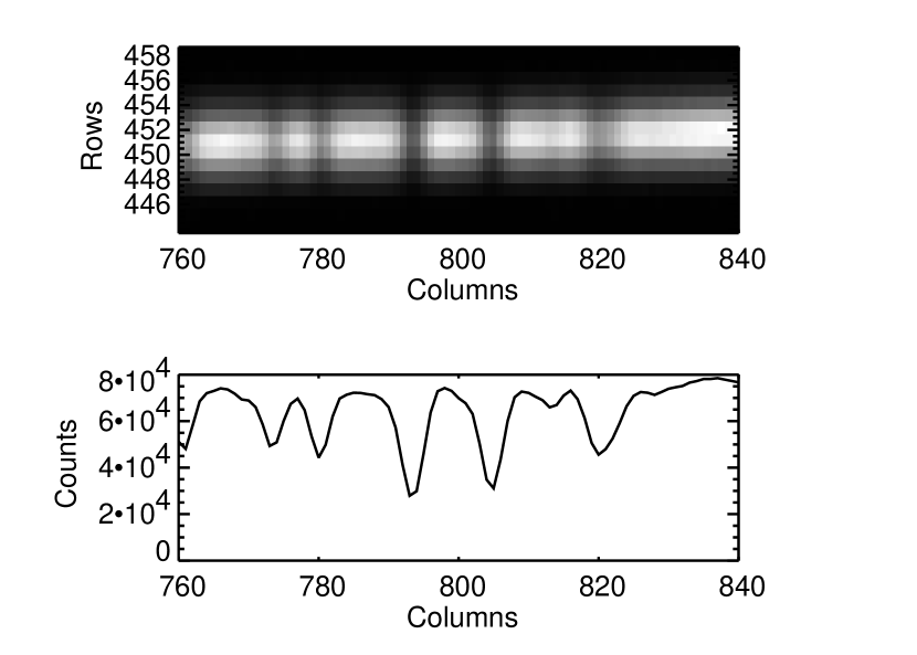
Figure 1: Top: A portion of a spectral order from a raw CCD image of the spectrum. Any emission line should span the full width of the stellar spectrum, as it is caused by seeing at the slit. Bottom: The reduction process converts a two dimensional spectrum into a one dimensional spectrum.

The recorded two–dimensional raw spectra are reduced in the usual way to one–dimensional spectra. The bias is subtracted from all images including both the stellar spectra and the flat–field exposures. Each spectral order recorded by the CCD has a width proportional to the diameter of the stellar seeing disk along the length of the slit. The typical seeing at Keck/HIRES of 0.7–1.2 arcsec yields orders of width $\sim$4 CCD rows (each “row” being the on–chip sum of neighboring original CCD rows). Cosmic rays are removed by searching for 7–$\sigma$ sharp intensity spikes at one row compared to the intensity in a neighboring row (at the same wavelength). We are indebted to Jason Wright for this cosmic–ray removal algorithm. The stellar spectra are divided by the flat–field exposures. The two–dimensional spectral orders are compressed to one dimension by summing the recorded counts within the $\sim$10 rows centered on each order. We thank Eric Nielsen for the careful reduction of CCD images. Figure 1 shows the results of this process. The signal–to–noise ratio per pixel in orders 72 through 89 of a typical 1-D spectrum is $\sim$200.

2.2 Overview of the Detection Scheme

We search for laser emission lines in the reduced spectra by comparing each spectrum to a reference spectrum of the same star, searching for statistically significant differences. Over time, a star’s spectrum should remain nearly constant except for minor fluctuations due to photon noise and photospheric changes. A large difference at one wavelength could signify the presence of a laser signal that had been detected during one observation but not during the other.

We would fail to detect an emission line if it occured at the same wavelength in both the observed and reference spectra. A laser fired continuously from the rest frame of the stellar photosphere would go undetected. However, such a continuous laser would be detected in both spectra at different wavelengths if the laser’s velocity vector were to change between observations, e.g. due to orbital motion around its host star. The resulting Doppler shift permit detections in the difference spectrum.

For each star, a series of algorithms is applied to all of its spectra. First a “reference” spectrum is chosen. Then, one by one, the other “test” spectra are aligned in wavelength with the reference for comparison (see §3.2). Candidate laser lines are found in the test spectra by subtracting the reference spectrum and searching for positive differences, or “spikes.” One test spectrum is then used as a secondary reference to check for spikes in the primary reference spectrum. The spikes are subjected to a selection criterion based on their width, to ensure that their shapes are consistent with the instrumental profile of HIRES (see §3.3). Spikes that are narrower than the instrumental profile are likely to be caused by cosmic rays hitting the CCD that eluded detection in the CCD reduction process described in §2.1.

A monochromatic laser line would have an intrinsic width narrower than the resolution of the spectrometer. However, as the laser light passes through the HIRES optical system, it would be smeared out by the HIRES point spread function (PSF), giving the detected emission line an apparent distribution in wavelength characteristic of the HIRES PSF. Thus candidate laser lines can be distinguished from most cosmic rays, most CCD flaws, and stellar emission lines by their predictable spread in wavelength that would be merely the HIRES PSF, as described in detail by Valenti et al. (1995). Notably, emission lines having widths that are narrower than possible from a star (with its thermal, collisional, turbulent, and rotational broadening mechanisms) would stand out as possibly “nonastrophysical” in origin. All of the resulting candidate emission lines of any width, excluding the apparent cosmic rays hits, from the spectra of each star are stored for further analysis as described in §4. In sections §3.1, §3.2, and §3.3, we describe in detail the processes by which we searched for emission lines.

2.3 Detection Limits for Laser Emission

To be detected, a laser signal must compete against the light of its host star. A laser beam carries three advantages over starlight. First, the laser light is concentrated in a narrow cone of tiny solid angle relative to starlight, which is omnidirectional. Second, a monochromatic laser line falls into one resolution element, with a width of $\sim$2.3 pixels, while starlight, composed of a wide range ($\sim$4000 Å) of wavelengths, is spread out into roughly 50,000 resolution elements. Lastly, the laser needs only to outshine the photon noise of the stellar flux, not the flux itself, within that resolution element since we are looking at differences in the spectra. To estimate these advantages of the laser signal, we consider the solid angles of the starlight and a diffraction–limited laser beam.

$$\Omega_{\rm star} = 4\pi$$ (1)

$$\Omega_{\rm laser} \approx \Bigg{(}{\lambda\over a}\Bigg{)}^{2}$$ (2)

Here $\lambda$ is the wavelength of the laser light and $a$ is the aperture size of the laser transmitter. The fraction of starlight contained within the laser beam is then given by

$$f_{\rm star}={1\over 4\pi}\Bigg{(}{\lambda\over a}\Bigg{)}^{2}$$ (3)

We note that the intrinsic width of a laser line will be much narrower than the HIRES resolution of $\sim$0.075 Å, thereby placing most all of the laser light into a single resolution element. The stellar spectral energy distribution may be approximated by a blackbody curve. For a Solar–type star, the SED has a width of $\sim$4000 Å, yielding the number of resolution elements, $N_{\rm star}$, into which the stellar luminosity falls:

$$N_{\rm star}\approx{4000\mbox{ \AA}\over 0.075\mbox{ \AA}}=5.3\times 10^{4}$$ (4)

The fraction of starlight contained within one resolution element is therefore given by

$$f_{\rm star,\mbox{ }\Delta\lambda}={1\over 4\pi}\Bigg{(}{\lambda\over a}\Bigg{)}^{2}{1\over 5.3\times 10^{4}}$$ (5)

The laser light needs only to outshine the stellar photon noise since we are detecting differences in a star’s spectrum over time. The photon noise relative to the flux itself, $\sigma$, for one spectrum is given by 1/(S/N) where S/N is the signal to noise ratio per resolution element. Since the laser must compete with the photon noise of two spectra in one resolution element, we have

$$\sigma\approx{\sqrt{2}\over\mbox{S/N}}$$ (6)

Finally we find that the laser power necessary for an $n\sigma$ detection is

$$P_{\rm laser}={1\over 4\pi}\Bigg{(}{\lambda\over a}\Bigg{)}^{2}{1\over 5.3\times 10^{4}}{n\sqrt{2}\over\mbox{S/N}}L_{\rm star}$$ (7)

where $L_{\rm star}$ is the luminosity of the star. As a representative case, we take $\lambda$=4500 Å, S/N=200, n=6, $L_{\rm star}=L_{\rm sun}=3.8~{}\times~{}10^{26}$ W, and assume Keck to Keck communication so $a$=10 m, which gives

$$P_{\rm laser}=50\mbox{ kW}$$ (8)

Thus for this representative case, one can detect a 50 kW laser.

The previous calculation assumes that the laser is on continuously. If, however, a nanosecond pulsed laser signal were transmitted, Equations 7 and 8 would need to be multiplied by the factor ${\Delta t_{\rm exp}\over{N_{\rm pulses}\times 10^{-9}\mbox{ s}}}$ where $\Delta t_{\rm exp}$ is the exposure time of the observation and $N_{\rm pulses}$ is the number of pulses received in that time. Using a typical exposure time of 10 minutes and assuming 1 pulse is received, the minimum necessary power of a detectable nanosecond pulsed laser is $P_{\rm pulsed}=3\times 10^{16}$ W. Thus, the minimum necessary energy of a detectable nanosecond pulsed laser is 30 MJ.

For comparison, the most powerful continuous laser on Earth is the Free Electron Laser (FEL) developed at Jefferson Laboratory in Virginia. The FEL has reached an average power of 1.7 kW and the laser is expected to achieve average powers up to $\sim$10 kW with an upgrade (Jefferson Lab 2001). Lawrence Livermore National Laboratory produced the world’s most powerful pulsed laser, the Petawatt laser. During its 440 femtosecond pulse, it delivered a power greater than 10¹⁵ W (LLNL 2001).

We can also determine a minimum detectable flux, $F_{\rm laser}$,

$$F_{\rm laser}={P_{\rm laser}\over A_{\rm laser}}$$ (9)

where $A_{\rm laser}$ is the area of the laser beam at the Earth and given by

$$A_{\rm laser}={\pi\over 4}\Bigg{(}{\lambda\over a}\Bigg{)}^{2}d^{2},$$ (10)

where $d$ is the distance from the laser to Earth. The flux limit can now be expressed as

$$F_{\rm laser}={4\over\pi}{1\over 5.3\times 10^{4}}{n\sqrt{2}\over\mbox{S/N}}{L_{\rm star}\over{4\pi d^{2}}},$$ (11)

where $L_{\rm star}/4\pi d^{2}$ is the flux of the star. If we take $d=100$ light years with the previously adopted values, the minimum flux of a detectable laser is

$$F_{\rm laser}=3.4\times 10^{-17}\mbox{ W/m${}^{2}$}$$ (12)

Thus, we can detect monochromatic laser light from nearby stars if the flux is at least $3.4~{}\times~{}10^{-17}$ W/m² at Earth.

3 Spectral Analysis

A detailed description of the algorithms developed to analyze the spectra is given in this section.

3.1 Choosing Reference Spectra

Two reference spectra are required for each star. The primary reference spectrum is compared to all the other test spectra. The second is compared to the primary reference spectrum. Since only positive differences are considered, any candidate laser lines in the first reference would not be flagged during its comparison with the test spectra. A second reference, one of the previous test spectra, is used to account for this possibility.

The two reference spectra are chosen as follows. Almost every star has at least one “template” spectrum. In the planet–search project, the stellar radial velocities are measured with respect to the template spectra. These observations are of good quality with high signal–to–noise ratios. If there are multiple–template spectra for a star, the two with the highest signal to noise are chosen as the reference spectra. If there is only one template, it is used as the primary reference spectrum and another observation with high signal to noise is chosen as the second reference. Some stars which are new to the extrasolar planet search catalog do not yet have templates. For these stars, the two observations with the highest signal to noise are chosen as the references.

3.2 Aligning Spectra

Aligning a pair of spectra precisely in both wavelength and flux is important. If the spectra are exactly the same, except for minor fluctuations due to photon noise, the fractional standard deviation, $\sigma$, of the difference spectrum is expected to be

$$\sigma=\sqrt{{1\over{\mbox{(S/N)}}_{1}^{2}}+{1\over{\mbox{(S/N)}}_{2}^{2}}}$$ (13)

where (S/N)₁ and (S/N)₂ are the signal–to–noise ratios of the two spectra. For two spectra with signal–to–noise ratios of 300, $\sigma$ can, in principle, be as low as 0.005. It is important to align the two spectra well enough such that the observed error is as close to the theoretical error as possible in order to detect the smallest differences.

We line up a pair of spectra order by order. Various normalization and shifting algorithms are applied to both the reference and test spectra, as follows. The first step is to put the orders on roughly the same flux scale by dividing by the continuum. The continuum is found by first partitioning an order into 10 bins. Each bin is assigned a temporary continuum at the 85th percentile in flux. A third–order polynomial is fit to these individual continua to normalize the entire spectral order.

Each spectrum is Doppler–shifted to correct for the Earth’s orbital motion, which causes a maximum wavelength shift of $\sim$1 Å  corresponding to $\sim$30 pixels. We determine the Doppler shift of the test spectrum relative to the reference spectrum by minimizing $\chi^{2}$, and then shift the test spectrum so that the two are aligned. The final shifts are precise to $\sim$0.01 pixel, and fractional pixel displacements of the spectra are accomplished with a spline interpolation. This shifting is first carried out on segments of length 280 pixels, and then it is done on a 40–pixel scale (“chunks”). If any spectrum contains cosmic rays (or laser emission lines), it is difficult to align. Such features are removed temporarily (replaced with a spline interpolation) to carry out the alignment. Operating on chunks of 40 pixels allows us to account for the wavelength dependence of the Doppler shift and to correct any slopes in the flux with wavelength.

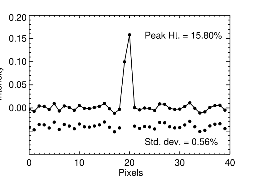
Figure 2: Top: A full chunk of difference spectrum, including spikes, which will be searched for laser line candidates. The peak height is 15.80% above the continuum. Bottom: The same chunk of difference spectrum with spikes removed and offset for clarity. The standard deviation of this spike-free chunk is the reported sigma.

The resulting (temporarily spike–free) reference and test spectra are subtracted to yield a difference spectrum, from which the standard deviation is determined and recorded as the “noise” for each spectral chunk. Finally the reference and test spectra are subtracted with all spikes included, leaving a difference chunk which can be searched for laser–line candidates. Figure 2 shows a chunk of difference spectrum both with (top) and without (bottom) flux spikes of unidentified origin.

3.3 Criteria for Laser Line Candidates

A laser beam would travel through the telescope and the HIRES spectrometer optics just as starlight would. Moreover, the laser beam travels through the same column of Earth’s atmosphere, acquiring the same wavefront distortions and seeing profile as does the star. Therefore, an emission line from a laser would span the whole width of a spectral order (perpendicular to dispersion) as would the stellar spectrum on the CCD. While the intrinsic width of the laser line in wavelength would be smaller than the resolution of HIRES, it would be broadened by the point–spread function of HIRES. The B1 slit used in HIRES projects to a width of 2.0 pixels on the CCD. The instrumental profile of HIRES from both its optics and the slit width is known from careful measurements (Valenti et al. 1995) and from simple Gaussian fitting of emission lines from a thorium-argon lamp. The instrumental profile with our HIRES setup has a width of 2.3 pixels (FWHM). Thus, we expect any laser line to have an observed width of 2.3 pixels.

We search for candidate emission lines in the stellar spectra as follows. Each 40–pixel chunk of difference spectrum has a corresponding fractional photon noise, $\sigma$, associated with it as described in §3.2. We pass through all the chunks and note spikes having heights above $6\sigma$. This threshold is chosen to exclude essentially all noise but detect a signal from a laser with the lowest detectable power.

We also require that candidate laser lines exhibit a width that is at least as broad as the HIRES instrumental profile, with FWHM=2.3 pixels, allowing us to discriminate against (i.e., reject) cosmic–ray hits. Most cosmic rays produce electrons in a single pixel or occasionally in two neighboring pixels, clearly narrower than the HIRES PSF. To implement this “width” criterion, we require that the shorter of the two adjacent pixels on either side of each 6–$\sigma$ spike contain at least 30% of the photons in that central spike. Examination of the known HIRES PSF and thorium comparison lines (see Figure 3) shows that this width criterion would be met by almost any emission line that had been broadened by the HIRES PSF. Any spike in the difference spectrum that does not meet both the 6–$\sigma$ height criterion and this width criterion is rejected from future consideration as they are probably cosmic rays. Spikes that do meet both criteria are stored in a database that includes the location and characteristics of that spike, for later statistical analysis (§4). We note that emission lines having widths greater than the PSF will be detected and stored as candidate signals. Thus our survey would detect intermittent emission lines of any origin, laser or astrophysical, if they are sufficiently strong.

4 Statistical Analysis of Candidates

The spectral analysis described in §3 yields a database of surviving candidate emission lines in each of the $\sim$12,500 Keck spectra of our 577 target stars. A typical star has $\sim$13 surviving candidate emission lines in its $\sim$20 spectra. For each candidate, the database contains the star, date of observation, the wavelength, the peak number of photons, and the width of the candidate line. Detailed examination shows that most (if not all) of the surviving candidate emission lines are simply cosmic ray hits that we had failed to reject.

To discriminate a true emission line from these cosmic rays, we apply a statistical analysis on the collection of emission–line candidates from all spectra (typically 20) for a given star. We search for an overabundance of candidates (“hits”) in the vicinity of any particular wavelength. In contrast, cosmic rays would hit at random locations on the CCD, and would not favor any particular wavelength. A clustering of hits near one wavelength from all the spectra of one star could indicate laser emission.

We note that the Earth’s orbital motion will not cause a Doppler shift of the laser line in our analysis, as we have already forceably shifted the reference and test stellar spectra onto the same wavelength scale (§3). However, acceleration of the emitter relative to the star (such as due to orbital motion) during the typical 4 years of observations would cause the laser line to be Doppler–shifted to neighboring wavelengths.

We make a grid representing the CCD with the spectral orders partitioned into approximately 30 segments of roughly 100 pixels each. The segments overlap one another by half of their size to account for the possibility of an abundance of hits split into two neighboring segments. We record the number of emission–line candidates in each segment.

For each star, we plot the number of 100–pixel segments against the number of hits in the segments. Most segments have no hits at all, and only a few have one hit. These infrequent hits (none or one hit out of $\sim$20 observations in a wavelength segment) are consistent with random cosmic ray hits. To this histogram, we fit a Poisson distribution (see Figure 4), and determine the probabilities of finding an excess number of hits, $n$, in any wavelength segment. A star exhibiting an excess number of hits in a segment, i.e. a low probability of the events occurring randomly, would stimulate further investigation as a potential emission line.

The fit of a Poisson distribution to the histogram of hits is done as follows. We fit the low–$n$ (0, 1, 2) portion of the histogram and neglect the high–$n$ tail. This approach avoids contaminating the Poisson mean, $\mu$, with actual emission lines in the high–$n$ tail. The first empty bin in the histogram, $n_{0}$, is determined and an estimate of the expected mean number of hits per segment, $\mu$, is calculated neglecting those segments with $n\geq n_{0}$.

The Poisson probability of finding $n$ cosmic ray hits in any given wavelength segment is given by (Taylor 1982):

$$P_{\mu}(n)=e^{-\mu}{\mu^{n}\over n!}$$ (14)

Using the estimated $\mu$, we calculate $P_{\mu}(n)$ for $n=0,1,...,n_{0}-1$, and check if any of the probabilities are less than 1%. If so, we exclude those bins from the fit as well if $n_{0}>2$. The fit is then applied to bins from $n=0$ to some $n_{\rm max}$ hits.

The estimated mean number of hits per segment may not necessarily yield a Poisson distribution that gives the best fit to the observed histogram. The best Poisson fit may be better determined by finding the lowest $\chi^{2}$ given by

$${\chi^{2}}=\sum_{n=0}^{n_{\rm max}}{(O_{n}-E_{n})^{2}\over E_{n}}$$ (15)

where $O_{n}$ is the observed number of segments containing $n$ candidate hits and $E_{n}$ is the expected number with $n$ hits, based on a Poisson distribution. The only free parameter is $\mu$, the mean number of hits per segment. We vary $\mu$ to find the value corresponding to the minimum of $\chi^{2}$. The resulting Poisson probabilities are multiplied by the total number of segments and adopted as the best fit to the observed histogram.

We now determine the probabilities of finding $n$ hits in any given segment, extrapolating beyond $n_{\rm max}$. Segments having an excessive number of hits with probabilities less than 0.01% are noted as serious candidate emission lines, as they occur in excess numbers above the background cosmic ray hits. Since there are about 500 wavelength segments on our grid of the CCD for each star, we expect to flag one in 20 stars spuriously, i.e. due to a chance coincidence of cosmic rays.

We find that indeed 45 stars were flagged as having a wavelength segment with an excess number of hits at the 0.01% false-alarm level. Each of the surviving flagged candidate laser lines, of which there were 187, were examined by eye in the raw CCD images.

5 An Apparent Emission–Line Detection

Our search for intermittent emission lines revealed an apparent detection for the star HD29528 (K0V). Three separate spectra obtained on different dates contained strong candidates at the same wavelength. The hits were noted in both of two overlapping spectral segments for this star. The probability that these three apparent emission lines were merely spurious cosmic rays occurring within a segment of length $\sim$200 km s^-1 is easily calculated from the Poisson occurrence of cosmic rays (§4).

Figure 4 shows the observed histogram of the number of segments versus number of hits along with the best fitting Poisson distribution. The probability of randomly obtaining 3 hits in a segment for this star is 1.23 $\times$ 10^-7 or 1 in 8 million.

Figure 5 shows these candidate laser lines in the reduced spectra of the three observations. The aligned reference and test spectra are shown and twice the difference spectra are below them. The candidate laser lines are in spectral order 83 and the central peaks are in pixel 1436 with respect to the reference spectrum.

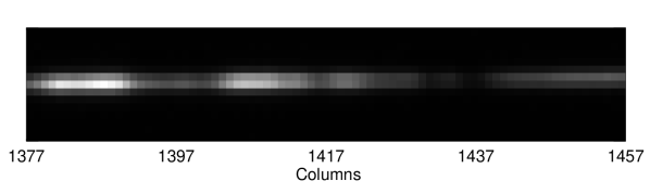
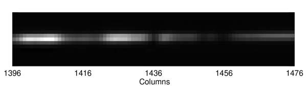
Figure 6: An apparent narrow emission line. Top: The raw CCD image of an observation of HD29528 taken on JD 2451793.1, centered on the first candidate laser line. Middle: The raw CCD image of the reference spectrum. Bottom: The difference of the two raw spectra. A bright line spanning the width of the spectral order can easily be seen.

We examined the raw spectra to see if the candidate laser lines span the whole width of the spectral order, indicating whether the light passed through the telescope and spectrometer. Figure 6 shows the raw CCD image of the spectrum of HD29528 obtained on JD 2451793.1, centered on the first candidate laser line. The reference spectrum is shown below it. Beneath the reference is the raw difference spectrum making it easier to see the apparent laser line. The other two candidate laser lines found in observations obtained on JD 2451882.98 and on JD 2451884.08 are not shown, but those apparent emission lines also span the width of the spectral order. Because all three hits occur at the same pixel (and hence wavelength) with respect to the star’s reference spectrum, and because they span the entire width of the spectral order, the hits are unlikely to be cosmic rays. These are surviving laser line candidates thus far in the analysis.

To further investigate these candidate emission lines in HD29528, we compared the spectrum of HD29528 to the solar spectrum using “The Solar Spectrum 2935 Å to 8770 Å” (Moore et al. 1966). The rest wavelengths of the lines are 4307.31 Å and there are no listed absorption lines due to the Earth’s atmosphere nor anomalous Solar emissions lines at this wavelength.

We further examined the spectrum of a rapidly rotating B–type star taken on the same night as the reference spectrum for HD29528. The B star spectrum should have no prominent spectral features. A strange drop in flux of 20% is seen in the spectrum, exactly at pixel 1436 in order 83, precisely where the hits were found with respect to the reference spectrum of HD29528 (see Figure 7). This clearly spurious feature in the B star strongly suggests that our candidate laser lines are merely artifacts caused by a flaw in the CCD.

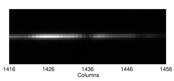
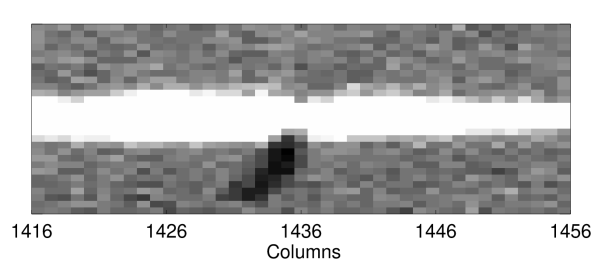
Figure 8: A flaw in the CCD masquerades as an emission line. Top: A chunk of raw spectrum from order 83 of the reference spectrum for HD29528 centered on the location of the candidate laser lines. Bottom: The same chunk of spectrum with the intensity levels adjusted. A dark CCD flaw can be seen under the bright spectral order.

Indeed, a close examination of the raw CCD image of the reference spectrum of HD29528 shows the flaw in the CCD (see Figure 8). This flaw is certainly the source of the false detection.

As a side note to this false detection of an emission line, one may calculate the necessary power of a laser that could have produced a “signal” similar to that detected. In Eqn 7 we assume a transmitter aperture, $a$=10 meters. The other variables are known. The wavelength of the 13$\sigma$ “signal” is 4307 Å, and the signal–to–noise ratio of the spectra is $\sim$120. The luminosity of a K0 star is 0.42 $L_{\rm sun}$ (Carroll and Ostlie 1996). Using these values in equations 7, we find $P_{\rm laser}=68$ kW. This would be the required power of a laser to produce the spurious signal in Figure 6. This test supports our expectation that lasers having power of 50 kW would have been detected.

6 Results

For each of the 45 stars that exhibited an excess of candidate emission lines (above the cosmic ray background noise) we examined the original raw CCD images from HIRES. Approximately 200 raw spectra were examined to follow up on the 45 flagged stars. Stellar emission lines were detected in the spectra of two flare stars, HIP5643 (M4.5) and HIP92403 (M3.5). Both stars exhibited varying emission of the Balmer line H$\beta$.

Interestingly, many candidate emission lines were located along the steep slopes of absorption lines in the reduced spectra. However, the corresponding emission spikes were not apparent in the raw CCD image. Such emission spikes are apparently neither cosmic rays nor emission lines. Instead, it is likely that these spikes located in absorption lines are caused simply by tiny changes in the instrumental profile of HIRES from one observation to the next. The changes in the instrumental profile could result from different atmospheric seeing of the star image at the slit (making the slit effectively a different size) or from small focus changes in HIRES itself. The steep sides of absorption lines have local intensities that are very sensitive to the instrumental profile. It is also possible that the spikes located in absorption lines are residual numerical artifacts from the spectral alignment process since interpolation routines normally give the largest errors on steep slopes. Thus these candidate emission spikes located within absorption lines were rejected as spurious.

All other candidate emission lines were visually inspected and found to be inconsistent with actual emission lines. Some were multiple, surviving cosmic rays that occurred, by chance, near the same wavelength. Some emission spikes were caused by bad pixels or flaws in the CCD. No lines consistent with laser emission were found in any of our stars.

7 Discussion

We would have detected time–varying emission lines from any of the 577 main sequence stars above a threshold of a few percent of the continuum flux. Emission lines of constant intensity would also have been detected had they Doppler–shifted relative to the star during the $\sim$4 yr of observations. Lines having intrinsic widths from arbitrarily narrow to tens of km s${}^{-1}~{}$would have been detected. No narrow lines consistent with laser emission were detected. However, naturally occurring emission lines were found in the spectra of two stars.

Emission lines in the spectra of Solar–type stars are rare between 4000 Å – 5000 Å. Such lines can arise occasionally in the chromospheres or coronae of the most magnetically active stars. In some ($\sim$20%) F, G, K–type main sequence stars, the cores of the Balmer absorption lines are “filled in” by a few percent due to chromospheric emission (Herbig 1985, Robinson, Cram, & Giampapa 1990). We would have detected temporal variation in that chromospheric filling, if it exceeded a few percent of the continuum level. No such variations were detected in any of our F, G, K–type main sequence stars. This nondetection indicates that such chromospheric variation in the cores of the strong Balmer lines, notably H$\beta$ and H$\gamma$, did not exceed a few percent of the continuum level in these stars. Flare stars, most of spectral type M0 or later, more commonly exhibit emission of H$\beta$. Indeed, we detected time–varying emission of H$\beta$ in two M–type flare stars.

Time–varying emission lines from stars may also arise from infalling volatile material and comets, as is observed for $\beta$ Pic (see for example Beust et al. 1998). Our search would have detected such astrophysical emission lines if they appeared or varied by more than a few percent of the continuum flux of the star. All such astrophysical origins for emissions lines would yield line widths greater than our resolution of 5 km s${}^{-1}~{}$due to the usual thermal and turbulent broadening, as well as possible rotational and collisional broadening. Hence such lines would be resolved. Nonetheless, no emission lines due to these effects were found in the 577 stars at our threshold of a few percent of continuum flux.

The entrance slit of the HIRES spectrometer is rectangular with dimensions 0.57 $\times$ 3.5 arcsec. At the typical distance of our stars of $\sim$50 pc, this slit corresponds to 30–175 AU at the star. Thus, sources of emission lines residing within 30 AU of our target stars would have been included in our spectra. Of course, the emission beam must be pointed toward the Keck telescope for detection. Extinction from interstellar dust is negligible toward these target stars due to their proximity ($d<$100 pc).

The motivation for this search stemmed from the suggestion of Schwartz and Townes (1961) that advanced civilizations might communicate from one colony to another within a planetary system, or from one planetary system to another, by using optical lasers as the carrier. The advantages of optical communication over radio include its higher bandwidth and its smaller diffraction beam to promote private communication.

A nondetection of extraterrestrial intelligence carries no value unless it excludes a plausible model of life in the universe. One might imagine the following model. The Milky Way Galaxy has an age of $\sim$10 Gyr, while only 4.6 Gyr were required to spawn a technological species on Earth. Approximately half of the stars in the Galactic disk are older than the Sun, and they formed with comparable amounts of heavy elements. Approximately 50% of these old disk stars do not have a stellar companion within 100 AU (Duquennoy and Mayor 1991), thereby permitting stable planetary orbits. Therefore, $\sim$25% of the stars in the Galactic disk have requisite characteristics of adequate age, chemical composition, and dynamical quiescence to serve as sites for the development of technological species. The anthropocentric nature of these stellar criteria are apparent, and thus serve merely as a useful guide for a model.

Coincidentally, the target stars used here are systematically middle–aged or older and void of close companions. They were selected for the Doppler planet search at Keck from among stars in the Solar neighborhood. They were chosen to have ages greater than 2 Gyr, as judged from the CaII H&K chromospheric emission line, because of the resulting photospheric stability of older stars. Moreover the target stars have no known stellar companions within 2 arcsec (typically $\sim$50 AU) to prevent any companion’s light from entering the spectrometer slit (but see Vogt et al. 2002 and Nidever et al. 2002 for a few recently detected, but negligibly bright, close companions). Moreover, spectroscopic analyses of the stellar spectra show that 90% of the target stars contain amounts of heavy elements that are within a factor of 2 of the Solar value ([Fe/H] = -0.3 to +0.3; D.A.Fischer, private communication).

Thus, the majority of the 577 target stars for this SETI search are older than the Sun, have roughly Solar chemical composition, and have no perturbing stellar companions within 50 AU. This stellar sample is clearly biased. Thus our observations test a limited model of the Galaxy in which older, single stars harbor technological civilizations.

The speculative model posits that some fraction of these target stars contain civilizations that sent probes to, or established colonies on, planets, moons or other platforms either in their host planetary system or in other systems. This model of behavior, albeit anthropocentric, stems from the tendencies of Homo Sapiens toward exploration. To communicate with such probes or colonies over distances of Astronomical Units to parsecs, some fraction of these civilizations might be modeled as using electromagnetic waves, including optical lasers.

We model the solid angle subtended by laser beams as follows. Some fraction, $f_{\rm tech}$, of the total number of target stars, $N_{\rm stars}$=577, harbor technological civilizations. On average each such civilization emits some number of laser beams, N_beams, perhaps in arbitrary directions. We consider that each beam subtends an average solid angle $\Omega_{\rm beam}$.

The total solid angle, $\Omega_{\rm Total}$, subtended by all arbitrarily oriented beams is

$$\Omega_{\rm Total}=N_{\rm stars}f_{\rm tech}N_{\rm beams}\Omega_{\rm beam}$$ (16)

We ignore here details of overlap of the beams, their actual distribution of power and beam size, and any purposeful aiming toward or away from us. Any properties of the lasers that are constructed with the Earth as a consideration could drastically change the probability of interception of such beams.

In our survey, we have monitored $N_{\rm stars}$= 577 stars. The nondetection obtained in the survey here suggests that the total solid angle subtended by lasers emitting 50 kW or more is constrained as $\Omega_{\rm Total}<4\pi$ sr .

Thus for arbitrarily directed beams, we constrain the model as

$$f_{\rm tech}N_{\rm beams}\Omega_{\rm beam}<4\pi/577$$ (17)

The nondetection reported here suggests lasers emitting detectable power must satisfy the above constraint for the combination of $f_{\rm tech}$, $N_{\rm lasers}$, $\Omega_{\rm beam}$. Apparently, advanced civilizations communicating by kilowatt optical lasers are not so common as to fill 4$\pi$ sr.

As a touchstone, we consider the case of the diffraction–limited laser with an aperture of 10-m (Keck–to–Keck), giving a solid angle for one beam, $\Omega_{\rm beam}\approx 10^{-15}$ sr. For transmitters of such aperture, a laser emitting 50 kW would be detectable. For this case, each star would have to emit $\sim 10^{13}$ arbitrarily oriented beams on average, each with power $P\geq$ 50 kW, in order that one would likely be oriented, serendipitously, toward us.

Clearly, the observed nondetection implies that such numerous, narrow beams, however implausible, do not exist in sufficient numbers to permit likely detection. These observations offer a poor constraint on lasers of arbitrary orientation, as their solid angles are simply too small in this model. One might consider a Galactic model consisting of wider laser beams, enhancing the chances of interception. In that case, the present nondetection would impose a constraint of fewer lasers emanating from the target stars, but would require proportionally higher power per laser for detection at 6–$\sigma$ above the stellar continuum.

More meaningfully, the nondetection reported here suggests that none of the 577 target stars harbors a civilization that has purposefully directed a laser with $P\geq$50 kW toward Earth (for the case of a 10–meter diffraction–limited transmitting aperture). This modest detection threshold of 50 kW highlights the ease with which an advanced civilization could signal us, if desired. But such is apparently not the case.

8 Acknowledgements

We thank the SETI Institute for generous funding of this work. We wish to thank R.Paul Butler and Steve Vogt for their endless hours in obtaining the Keck/HIRES spectra. S.Vogt’s design of HIRES made this work possible. We thank Jason Wright for the new CCD reduction algorithm of Keck spectra that efficiently removed cosmic ray hits. We thank Eric Nielsen for reducing the 12,500 CCD images to one–dimensional spectra. We thank Debra Fischer for chemical–abundance measurements of the target stars. We also thank D.Nidever, D.Werthimer, J.Tarter, F.Drake, M.Lampton, B.Walp and referee, William D. Cochran for many useful comments. This work was carried out by A.R. as partial fulfillment of the of the requirements toward a Master’s Degree in physics at San Francisco State University.

Figure 3: Emission lines in a thorium-argon spectrum showing the spectrometer PSF.

Figure 4: The observed histogram of the number of segments versus number of hits for the star HD29528. The dots indicate the best fitting Poisson distribution with the mean number of hits per segment equal to 0.00907.

Figure 5: Three hits in the reduced spectra of HD29528. The test spectra (dotted lines) have been aligned with the reference spectra (solid lines). Twice the difference spectra are shown below. The candidate laser lines are in order 83 and the central peak is in pixel 1436 with respect to the reference spectrum.

Figure 7: Top: Order 83 of a B star spectrum. A strong feature can be seen at pixel 1436. Bottom: Zooming in on the bad pixels.

References

- (1) Beust H., Lagrange A.-M., Crawford I.A., Goudard C., Spyromilio J., Vidal-madjar A. 1998, AA, 338, 1015 The beta Pictoris circumstellar disk. XXV. The CaII absorption lines and the Falling Evaporating Bodies model revisited using UHRF observations.
- (2) Bhathal, R. 2000, in Bioastronomy 99: A New Era in Bioastronomy, eds. G. Lemarchand & K. Meech, ASP Conf. Proc., vol. 213, 553.
- Butler et al. (2000) Butler, R. P., Vogt, S. S., Marcy, G. W., Fischer, D. A., Henry, G. W. & Apps, K. 2000, ApJ, 545, 504.
- (4) Carroll, B. and Ostlie, D. 1996, in An Introduction to Modern Astrophysics, Addison-Wesley Publishing.
- (5) Cullers, K. 2000, in Bioastronomy 99: A New Era in Bioastronomy, eds. G. Lemarchand & K. Meech, ASP Conf. Proc., vol. 213, 451.
- (6) Duquennoy, A. and Mayor, M. 1991, A&A, 248, 485
- (7) Herbig, G. H. 1985, ApJ, 289, 269
- (8) Howard, A., Horowitz, P., Coldwell, C., Klein, S., Sung, A., Wolff, J., Caruso, J., Latham, D., Papaliolios, C., Stefanik, R., & Zajac, J. 2000, in Bioastronomy 99: A New Era in Bioastronomy, eds. G. Lemarchand & K. Meech, ASP Conf. Proc., vol. 213, 545.
-
(9)
Jefferson Lab. 2001. “Free-Electron Laser Program.”
Obtained 6 January 2002
http://www.jlab.org/FEL/feldescrip.html. - (10) Lampton, M. 2000, in Bioastronomy 99: A New Era in Bioastronomy, eds. G. Lemarchand & K. Meech, ASP Conf. Proc., vol. 213, 565.
- (11) Lawrence Livermore National Laboratory (LLNL). 2001. “The Amazing Power of the Petawatt.” Obtained 6 January 2002 http://www.llnl.gov/str/MPerry.html.
- (12) Leigh, D. and Horowitz, P. 2000, in Bioastronomy 99: A New Era in Bioastronomy, eds. G. Lemarchand & K. Meech, ASP Conf. Proc., vol. 213, 459.
- (13) Moore, E., Minnaert, M. G. J., Houtgast, J. 1966, in The Solar Spectrum 2935 Å to 8770 Å. National Bureau of Standards Monograph 61.
- (14) Nidever, D., Marcy, G. W., Butler, R. P., Fischer, D. A., Vogt, S. S. 2002, submitted to ApJ Supp.
- (15) Reines, A. E. 2001, Master’s thesis, San Francisco State University
- (16) Robinson, R. D., Cram, L. E., Giampapa,M. S. 1990, ApJS, 74,891
- (17) Schwartz, R. M. and Townes, C. H. 1961, Nature, 190, 205.
- (18) Tarter, J. 2001, ARAA, 39, 511-548.
- (19) Taylor J. R. 1982, in An Introduction to Error Analysis: The Study of Uncertainties in Physical Measurements, University Science Books, ch. 11 & 12.
- (20) Townes, C. 1997, in Proc. 5th Int. Conf. on Bioastronomy, eds. C. Cosmovici, S. Bowyer, & D. Werthimer., IAU Colloq. No. 161, 585.
- Valenti et al. (1995) Valenti, J. A., Butler, R. P., & Marcy,G.W. 1995, PASP, 107, 966.
- Vogt et al. (1994) Vogt, S. S. et al. 1994, Proc. Soc. Photo-Opt. Instr. Eng., 2198, 362
- Vogt et al. (2000) Vogt, S. S., Marcy, G. W., Butler, R. P., Apps, K. 2000, ApJ, 536, 902
- Vogt et al. (2002) Vogt, S. S., Butler, R. P., Marcy, G. W., Fischer,D.A., Pourbaix,D., Apps, K., Laughlin,G. 2002, Accepted for publication, ApJ
- (25) Werthimer, D., Bowyer, S., Cobb, J., Lebofsky, M., Lampton, M. 2000, in Bioastronomy 99: A New Era in Bioastronomy, eds. G. Lemarchand & K. Meech, ASP Conf. Proc., vol. 213, 479.
- (26) Werthimer, D., Anderson, D., Bowyer, S., Cobb, J., Heien, E., Korpela, E., Lampton, M., Lebofsky, M., Marcy, G., McGarry, M., & Treffers, D. 2001, in The Search for Extraterrestrial Intelligence in the Optical Spectrum III, ed. S. Kingsley, Proc. of SPIE, vol. 4273