The Intrinsic Shapes of Molecular Cloud Fragments over a Range of Length Scales

Abstract

We decipher intrinsic three-dimensional shape distributions of molecular clouds, cloud cores, Bok globules, and condensations using recently compiled catalogues of observed axis ratios for these objects mapped in carbon monoxide, ammonia, through optical selection, or in continuum dust emission. We apply statistical techniques to compare assumed intrinsic axis ratio distributions with observed projected axis ratio distributions. Intrinsically triaxial shapes produce projected distributions which agree with observations. Molecular clouds mapped in ¹²CO are intrinsically triaxial but more nearly prolate than oblate, while the smaller cloud cores, Bok globules, and condensations are also intrinsically triaxial but more nearly oblate than prolate.

1 Introduction

Numerous catalogues have now compiled properties of hundreds (or even thousands) of molecular clouds or cloud fragments with a large range of sizes, allowing meaningful statistical analysis of properties of molecular clouds, cloud cores, and smaller condensations. With such data sets, the distribution of apparent projected core axis ratio $p$ can be used to constrain the intrinsic three-dimensional shapes. In a previous paper (Jones, Basu, & Dubinski 2001; hereafter Paper I), we investigated the shapes of molecular cloud cores mapped in NH₃ (Jijina, Myers, & Adams 1999) and cores mapped through optical selection (Lee & Myers 1999) via both statistical and analytical methods. We found that strictly axisymmetric prolate or oblate shapes cores could not reproduce the observed projected axis ratios and that molecular cloud cores were triaxial.

In this paper, we extend our previous work and conduct a statistical analysis of seven recent data sets which include a wide range of sizes of objects, from molecular clouds with effective radius as large as 45 pc (Heyer, Carpenter, & Snell 2001) to submillimeter dust continuum maps of condensations with major axes as small as 2800 AU, or $\sim 0.01$ pc (Motte et al. 2001). The information obtained about the intrinsic shapes of these objects can yield insight into the physical processes which govern their evolution and subsequent star formation. We examine the ¹²CO catalogue of molecular regions in the outer Galaxy compiled by Heyer et al. (2001) in § 3.1, cores mapped in NH₃ and C¹⁸O in § 3.2 (Onishi et al. 1996; Tachihara, Mizuno, & Fukui 2000), catalogues of Bok globules (Clemens & Barvainis 1988; Bourke et al. 1995) in § 3.3, and millimeter and submillimeter continuum maps of smaller protostellar condensations (Motte, André, & Neri 1998; Motte et al. 2001) in § 3.4. A discussion and summary are given in §§ 4 and 5.

2 Methods

In general, a triaxial ellipsoid can be described by the equation

$$x^{2}+\frac{y^{2}}{\zeta^{2}}+\frac{z^{2}}{\xi^{2}}=a^{2},$$ (1)

where $a$ is a constant and $1\geq\zeta\geq\xi$. The geometrical analysis of Stark (1977) and Binney (1985) shows that such a body, when viewed in projection, has elliptical contours. Following Binney (1985), the projection of a triaxial body when viewed from an observing angle $(\theta,\phi)$ (where the angles are defined on an imaginary viewing sphere and have their usual meaning in a spherical coordinate system) is found using the quantities

$$A\equiv\frac{{\cos}^{2}\theta}{\xi^{2}}\left({\sin}^{2}\phi+\frac{{\cos}^{2}\phi}{\zeta^{2}}\right)+\frac{{\sin}^{2}\theta}{\zeta^{2}},$$ (2)

$$B\equiv\cos\theta\,\sin 2\phi\left(1-\frac{1}{\zeta^{2}}\right)\frac{1}{\xi^{2}},$$ (3)

and

$$C\equiv\left(\frac{{\sin}^{2}\phi}{\zeta^{2}}+{\cos}^{2}\phi\right)\frac{1}{\xi^{2}}.$$ (4)

The apparent axis ratio in projection then equals

$$p={\left(\frac{A+C-D}{A+C+D}\right)}^{1/2},$$ (5)

where $D\equiv\sqrt{{\left(A-C\right)}^{2}+B^{2}}$. Using these equations, one can construct probability distributions for the projected axis ratio, assuming a large number of randomly distributed viewing angles.

We assign a Gaussian distribution of values for each axis ratio $\zeta$ and $\xi$, with a mean in the range $[0,1]$, and standard deviation $\sigma$ typically equal to 0.1, consistent with our use of 10 bins to sample the data. We did test a range of $\sigma$ from 0.05 to 0.2, and find that our conclusions do not change significantly within this range (see discussion in § 4). The drawback to using $\sigma\gtrsim 0.2$ is that a relatively large fraction of the Gaussian distribution can fall outside the allowed range $[0,1]$. For example, a Gaussian distribution centered at 0.8 with a $\sigma$ of 0.2 has $\approx$ 16% of the data $>1$ (see Paper I for an extended discussion of this issue). For similar reasons, we limit the $\sigma=0.1$ analysis to the range of axis ratios [0.1, 0.9].

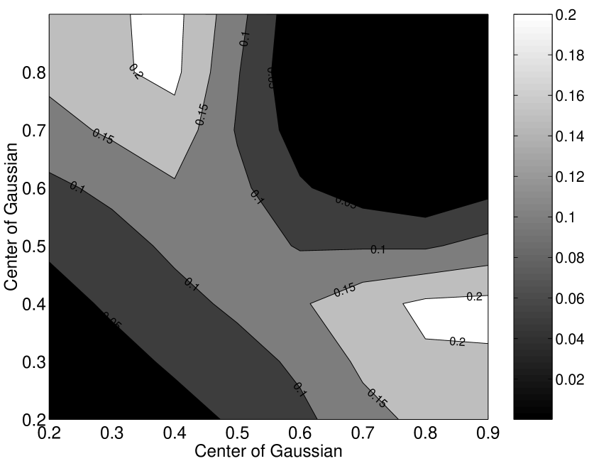
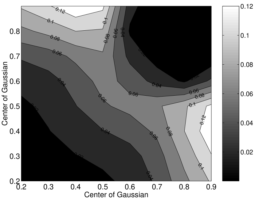
In order to find the best fit intrinsic distribution of triaxial bodies, distributions of axis ratios with peak values $\xi_{0}$ and $\zeta_{0}$ (for a given $\sigma$) are input into a Monte Carlo program. We typically employ at least $10^{4}$ viewing angles to calculate the projected distribution for each individual pair of axis ratios, and at least $10^{4}$ sets of axis ratios for each Gaussian distribution. This is more than sufficient for comparison with data sets sampled in 10 bins. The program produces the expected observed distribution which results from the assumed intrinsic distributions. We compare this output with the observed data sets via their $\chi^{2}$ values calculated by comparing the area of each bin to the area under the expected distribution at the location of each bin. Distributions of triaxial shapes for which the mean values $\xi_{0}=\zeta_{0}$ emphasize prolate objects, while those distributions with $\zeta_{0}$ near 1 emphasize oblate objects. Furthermore, distributions with $\zeta_{0}>\text@frac{1}{2}(1+\xi_{0})$ can be classified as containing more nearly oblate than prolate objects. For greater details consult Paper I.

3 Results

3.1 Molecular Clouds

Heyer et al. (2001) have catalogued the properties of clouds and clumps using ¹²CO data from a survey of the outer Galaxy. The catalogue consists of $10\,156$ objects which include small, isolated clouds and clumps within larger clouds. Observations from the outer Galaxy have the advantage that there is no distance ambiguity and the clouds are more widely spaced along the line of sight which eliminates problematic blending of emission, allowing cloud properties to be determined more accurately. The FWHM beam size for this catalogue is $45^{{}^{\prime}\!{}^{\prime}}$ and there are an impressive $10\,134$ objects with major and minor axes tabulated. Heyer et al. (2001) point out that the largest clouds, with effective radius $r_{\rm e}$ of about 10 pc or larger, are self-gravitating, whereas the smaller clouds (comprising the vast majority of observed objects) are not self-gravitating. This boundary also approximates the usual distinction between molecular clouds and giant molecular clouds, or GMC’s (see Blitz 1991; Williams, Blitz, & McKee 2001).

Given the evidence for a physical distinction based on size, we performed our analysis on the entire data set as well as a subset with $r_{\rm e}>10$ pc, which corresponds to a mass range of approximately $\sim 10^{4}\>\rm{to}\>10^{5}\>\rm{M}_{\odot}$, typical of GMC’s. Furthermore, to avoid any pathological cases where an elliptical fit to the cloud shape can be a very poor approximation (M. H. Heyer, 2001, private communication), we restricted our sample to those clouds which span at least 10 spatial pixels in the observations (an even more restrictive threshold of 20 pixels also yields essentially the same final result). This criterion reduces the total set to 5685 and the subset of GMC’s to 85. Our separate analyses can reveal whether there is any significant shape difference in the two populations.

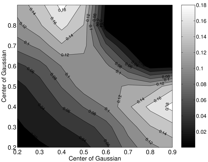
Figure 1 shows the results of the $\chi^{2}$ calculations for the triaxial fitting of the GMC subset. The data set is best fit by distributions with axis ratios $(\xi_{0},\zeta_{0})=(0.2,0.2)$ when $\sigma=0.1$. In order to determine whether values of $(\xi_{0},\zeta_{0})$ closer to zero would improve the fit, we repeated the analysis with a value of $\sigma=0.05$. (As the mean value of the Gaussian gets closer to the endpoints of the allowed range [0,1], a larger fraction of the Gaussian distribution falls outside this range, for a given $\sigma$. There is no ideal way to correct for this problem as explained in § 2 of this paper and in § 4 of Paper I). However, even with $\sigma=0.05$, the best fit mean axis ratios $(\xi_{0},\zeta_{0})$ are not closer to zero and agree with our result for $\sigma=0.1$ within the estimated error. See § 4.1 for a discussion of the errors which we estimate to be a maximum of $\pm\,0.1$ in the mean value of each axis ratio.

Figure 1: Two-dimensional plot of inverse $\chi^{2}$ values for triaxial core shape models applied to clouds with effective radius greater than 10 pc (and observed with at least 10 pixels) in the catalogue of Heyer et al. (2001). Note the symmetry of the figure about the line along which the two centers of the axis distributions are equal. For any point in the figure, the smaller axis ratio corresponds to $\xi_{0}$ and the larger to $\zeta_{0}$.

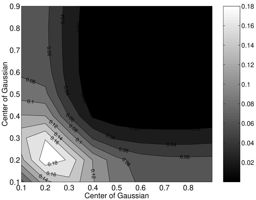
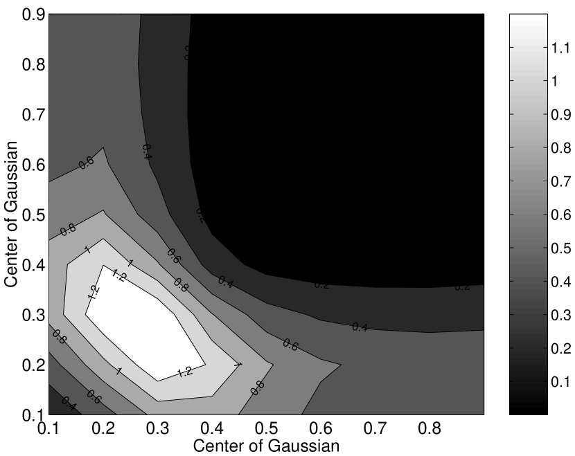
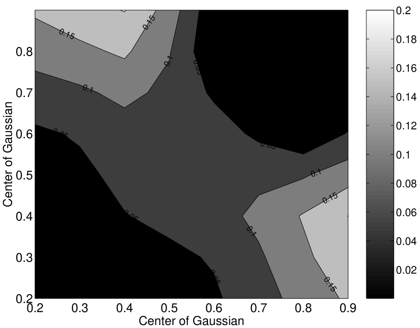
Figure 2 shows the result of the $\chi^{2}$ calculation for the complete set of axis ratios based on our selection criteria in the Heyer et al. (2001) catalogue. The best fit based on the $\chi^{2}$ values is $(\xi_{0},\zeta_{0})=(0.3,0.3)$.

For both the total set and for the subset based on large effective radius, the best-fit triaxial distributions require $\xi_{0}=\zeta_{0}$, as shown very clearly in Figure 1 and Figure 2. This means that the distributions emphasize prolate objects. However, since $\xi_{0}$ and $\zeta_{0}$ are the means of distributions, most individual objects cannot be considered strictly prolate and are, in fact, triaxial. For the clouds with large $r_{\rm e}$, the distributions which best fit the observations have thinner objects (smaller $\xi$ and $\zeta$) than those that best fit the entire set. However, the difference is quite small and equal to our maximum estimated error of $\pm\,0.1$.

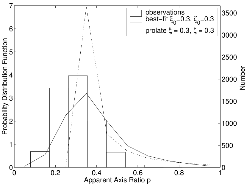
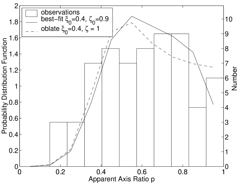
Figure 3 compares the best fit distribution of $p$ to the complete binned data set of Heyer et al. (2001). It also reveals that the histogram of projected shapes $p$ of molecular clouds has some unique features. We recall that our previous analysis (Paper I) of dense cores showed that an observed broad peak in the distribution at $p\gtrsim 0.5$ and the presence of a significant number of objects near $p=1$ favored triaxial, but more nearly oblate intrinsic shapes. Indeed, this pattern is reinforced in our subsequent study of other cores, Bok globules, and protostellar condensations (see § 3.2 - 3.4). However, the shapes of molecular clouds are distinct in that they have a very narrow peak, and at a low value $p\approx 0.3$. The narrow peak favors near-prolate objects, although a pure prolate cloud with $\xi=\zeta=0.3$ yields a poor fit to the data, as shown in Figure 3. A pure prolate cloud would have too narrow a peak in the observed shape distribution, as well as a higher probability than observed of a near-circular projection (see discussion and figures in § 2 of Paper I). In fact, Figure 3 shows that even a Gaussian distribution of triaxial objects implies a higher probability of detecting near-circular objects than observed.

The cutoff in high values of $p$ may be due to an actual cutoff in the distribution of intrinsic axis ratios $(\xi_{0},\zeta_{0})$ above some value, or could be due to some selection effect. One selection effect in the Heyer et al. (2001) sample is the fact that an object must span at least 5 pixels in the map to be classified as a cloud (additionally, we impose the higher threshold of 10 pixels for our shape analysis). However, we see no evidence in the sample for a trend toward greater circularity as clouds have smaller projected size. Another selection effect is that the edges of the objects in the sample likely correspond to the the CO photodissociation boundary and not that of the H₂ gas (Heyer et al. 2001). However, it is again not clear that this in any way biases against near-circular objects.

Figure 2: Two-dimensional plot of inverse $\chi^{2}$ values for triaxial core shape models applied to the entire catalogue of Heyer et al. (2001) based on our selection criterion.

Figure 3: Comparison of the observed axis ratios from Heyer et al. (2001) with the best fit assuming triaxial clouds (solid line) and assuming a pure prolate cloud (dot-dashed line). The actual number of observations in the bins is shown on the right-hand side vertical axis.

3.2 Dense Cores

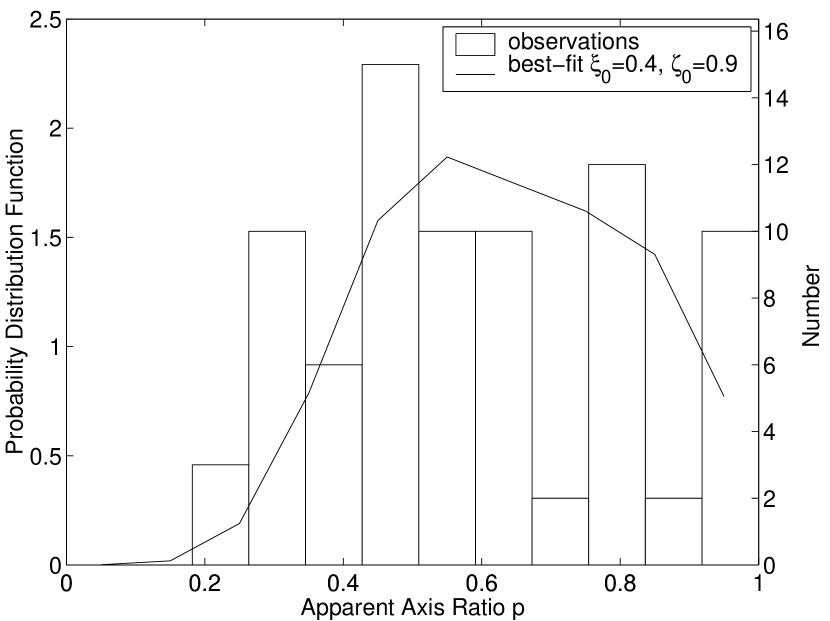
Onishi et al. (1996) and Tachihara et al. (2000) have observed dense cloud cores in Taurus and Ophiuchus, respectively, in C¹⁸O with telescopes at Nagoya University. Since the same telescopes and technique were used to obtain these ratios, and both groups quote the axial ratios to a tenth of a parsec, we combined these two surveys in order to obtain a reasonable sized set for statistical analysis. The final set of data from these two regions includes 80 cores. The best fit determined by calculating the $\chi^{2}$ values is $(\xi_{0},\zeta_{0})=(0.4,0.9)$; see Figure 4. The best fit is compared with the binned data set in Figure 5. We performed this analysis with and without the sources for which there were embedded IR sources and obtained the same result.

Although our best fit underestimates the observed axis ratios in the bin near $p=1$, it also overestimates the previous bin. The significant bin to bin variation is likely due to the relatively small size of this sample. However, the best fit agrees within the estimated errors, with the results presented in Paper I using much larger samples of NH₃ data (Jijina et al. 1999) and optical data (Lee & Myers 1999) for dense cores. Jijina et al. (1999) catalogued core properties for 264 objects from NH₃ observations and Lee & Myers (1999) catalogued properties for 406 dense cores from contour maps of optical extinction. The Jijina et al. data set is best fit by triaxial distributions with mean axis ratios $(\xi_{0},\zeta_{0})=(0.5,0.9)$, and the Lee & Myers data set is best fit by mean values $(\xi_{0},\zeta_{0})=(0.3,0.9)$.

Figure 4: Two-dimensional plot of inverse $\chi^{2}$ values for triaxial core shape models applied to the combined surveys of Onishi et al. (1996) and Tachihara et al. (2000).

Figure 5: Comparison of the observed axis ratios from Onishi et al. (1996) and Tachihara et al. (2000) with the best fit assuming triaxial cores (solid line). The actual number of observations in the bins is shown on the right-hand side vertical axis.

3.3 Bok Globules

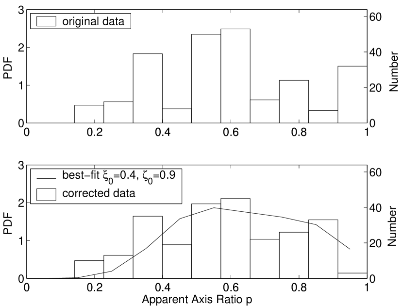
Bourke et al. (1995) catalogued physical characteristics of 169 isolated small molecular clouds (Bok globules) in NH₃ from the southern sky. These observations were compiled to complement a similar study of 248 optically selected Bok globules in the northern hemisphere by Clemens & Barvainis (1988). We note that Clemens & Barvainis (1988) also found that there was no correlation between the orientation of the clouds relative to the Galactic plane and their projected optical shapes. Ryden (1996) looked at the shapes of the globules from these two data sets based on the assumption of axisymmetry. She found that the Bok globules were consistent with oblate objects having an intrinsic mean axis ratio $q=0.3$, or prolate objects having $q=0.5$. Ryden (1996) realized that these sets suffered from rounding errors. This affected the smallest major and minor axes, yielding an artificially large number of axis ratios near one. For example, Clemens & Barvainis (1988) measured the Palomar Observatory Sky Survey plates to compile their catalogue. They rounded the major and minor axes to the nearest millimeter, which corresponds to an angular size of $1^{{}^{\prime}}\!.12$. The set is comprised of a relatively large number of small globules (42 out of 248) which have a major axis less than 2 mm. When these smallest values are rounded, the result is a large number of axis ratios erroneously equal to one or close to one. The top panel of Figure 6 shows very clearly that there are proportionally a large number number of objects in the bin with the largest axis ratios. Obviously, this problem does not affect the larger globules as significantly. Ryden (1996) compensated for this problem by adding to each of the original major and minor axes a random error term $\Delta$. She did this hundreds of times and obtained a new distribution of major and minor axes by taking an average from all her trials. See Ryden (1996) for additional details. We followed her procedure to correct for these rounding errors and obtained a new distribution of axis ratios for both data sets. Since the roundoff error is likely selected uniformly from within a fixed range, we used a random number generator to select uniformly from a prescribed range of estimated error. For the Clemens & Barvainis (1988) and the Bourke et al. (1995) data sets, we used a range of error $-0^{{}^{\prime}}\!.56<\Delta<+0^{{}^{\prime}}\!.56$, and $-0^{{}^{\prime}}\!.25<\Delta<+0^{{}^{\prime}}\!.25$, respectively. Figure 6 shows both the original binned data of axis ratios and the corrected distribution of axis ratios for the Clemens & Barvainis (1988) data. Notice that the large number of axis ratios near one in the original set has been dramatically reduced. We investigated these two sets and found that intrinsic triaxial shapes produced distributions which agreed with the observations. Figure 7 and Figure 8 show the results of the $\chi^{2}$ calculations with the triaxial fitting for the Clemens & Barvainis (1988) and the Bourke et al. (1995) corrected data sets, respectively. The Clemens & Barvainis (1988) data set is best fit by distributions with mean axis ratios $(\xi_{0},\zeta_{0})=(0.4,0.9)$, and the Bourke et al. (1995) data set is also best fit by mean values $(\xi_{0},\zeta_{0})=(0.4,0.9)$. The best fit for the Clemens & Barvainis (1988) data is also shown in Figure 6.

Figure 6: Clemens & Barvainis (1988) original binned normalized data set and the same data corrected for rounding errors. The original and corrected data are displayed in the top and bottom frames, respectively. The black solid line is the best fit from the triaxial distributions. The actual number of objects in the bins is shown on the right-hand side vertical axis.

Figure 7: Two-dimensional plot of inverse $\chi^{2}$ values for triaxial core shape models applied to the catalogue of Clemens & Barvainis (1988) with the rounding errors corrected.

Figure 8: Two-dimensional plot of inverse $\chi^{2}$ values for triaxial core shape models applied to the catalogue of Bourke et al. (1995) with the rounding errors corrected.

3.4 Condensations Mapped in Millimeter-Submillimeter Wavelengths

Motte et al. (1998) observed the $\rho$ Ophiuchi main cloud at 1.3 mm with the IRAM 30 m telescope and were able to detect 58 individual compact dusty objects with a fragmentation size scale of approximately 6000 AU. After we removed clumps which were thought to be composite in nature, there were 35 clumps for which projected major and minor axes were resolved. Although this is a small sample for statistical analysis, we still present the results of the $\chi^{2}$ calculations from the triaxial fitting in Figure 9. The Motte et al. (1998) data set is best fit by distributions with mean axis ratios $(\xi_{0},\zeta_{0})=(0.4,0.9)$.

Figure 9: Two-dimensional plot of inverse $\chi^{2}$ values for triaxial core shape models applied to the survey of Motte et al. (1998) with the composite clumps removed.

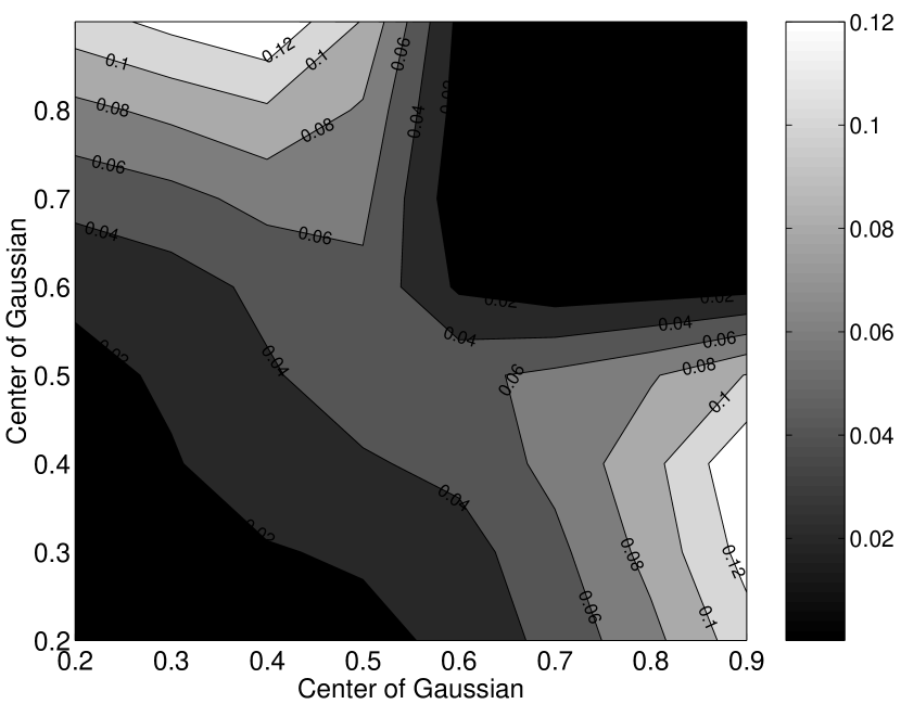
Motte et al. (2001) surveyed the protoclusters NGC 2068 and NGC 2071 in Orion B at 850 $\mu$m and 450 $\mu$m with SCUBA (Submillimeter Common User Bolometer Array) on the JCMT and were able to detect small objects (size $\sim$ 5000 AU) which they call condensations. There were 64 condensations for which the projected major and minor axes were obtained. This is a remarkable data set which measures objects on size scales approaching that of our solar system. The results of the $\chi^{2}$ calculations with the triaxial fitting are presented in Figure 10 for $\sigma=0.1$. The Motte et al. (2001) data set is best fit by distributions with mean axis ratios $(\xi_{0},\zeta_{0})=(0.4,0.9)$. Since the binned observed data of axis ratios does not have a strong peak, but instead looks rather flat, we repeated our analysis for $\sigma=0.2$. For $\sigma=0.2$, the data set is best fit by distributions with mean axis ratios $(\xi_{0},\zeta_{0})=(0.5,0.9)$. However, the distribution with the mean value of 0.9 and $\sigma=0.2$, has $31\%$ of the data values outside the allowed range. After the data is truncated, the remaining distribution will not have a final mean at 0.9 and $\sigma=0.2$, and the remaining values inside the allowed range must also be normalized. As a result, the normalized distribution is actually peaked more than one would intuitively expect. Consequently, the $\chi^{2}$ values for $\sigma=0.2$ are no better than the $\chi^{2}$ values for $\sigma=0.1$. The best fit for $\sigma=0.1$ is compared with the observed data in Figure 11.

Interestingly, Figure 11 shows that there are a number of objects with an apparent axis ratio near or exactly equal to one. A close examination of the original Motte et al. (2001) data reveals that the objects which fall into this bin are well above the resolution limit and that this large number is not a selection effect. Since this data set has a number of axis ratios near $p=1$, it is interesting to speculate whether or not intrinsic oblate objects (rather than near-oblate triaxial objects) may agree with the observations. We used two additional tests to investigate this hypothesis. First, we fit the histogram of observed shapes with a curve and carry out an analytic inversion to see if it is consistent with a distribution of intrinsic oblate shapes. The resulting intrinsic shape distribution $\psi(q)$ does go negative near $q=1$ just as in the inversions performed on the dense core shape data of Jijina et al. (1999) and Lee & Myers (1999) in Paper I. This is due to the continuing presence of a decline in the observed axis ratio distribution $\phi(p)$ towards $p=1$. To investigate further, we also experiment with an intrinsic axis distribution that is Gaussian in $\xi$, with $\xi_{0}=0.4$ and $\sigma=0.1$, but has a fixed value $\zeta=1$ for all clouds, i.e., the clouds are all oblate with various degrees of flattening. In this case, our Monte Carlo program yields a probability distribution function which is plotted in Figure 11. The inverse $\chi^{2}$ values for both the pure oblate objects and the best fit triaxial objects are $\approx 0.2$. The Motte et al. (2001) data, unlike the dense core data presented or reviewed in § 3.2, is close enough to being flat near $p=1$ and has a small enough sample of objects that we cannot entirely exclude the pure oblate hypothesis on the basis of the $\chi^{2}$ test. If just one of the six objects (interestingly, one object has an embedded class 0 protostar) is removed from the bin closest to $p=1$, the near-oblate triaxial objects provide a much better fit. Further observations and a larger sample will be necessary before the intrinsic shapes of these very dense objects can be determined with certainty. Nevertheless, we can conclude that molecular cloud condensations are either oblate or near-oblate in shape.

Figure 10: Two-dimensional plot of inverse $\chi^{2}$ values for triaxial core shape models with $\sigma=0.1$ applied to the survey of Motte et al. (2001).

Figure 11: Comparison of the observed axis ratios from Motte et al. (2001) with the best fit assuming triaxial cores for $\sigma=0.1$ (solid line) and assuming pure oblate cores (dashed line). The actual number of observations in the bins is shown by the right-hand side vertical axis.

4 Discussion

4.1 Error Bounds

In order to test the reliability of our results we recalculate the $\chi^{2}$ values after randomly removing $20\%$ of the data and repeat this procedure ten times for each set. For every set investigated in this paper we obtain the same best fit mean axis ratios $(\xi_{0},\zeta_{0})$ for all the trials with the exception of two trials with the Motte et al. (1998) data. This data set has only 35 non-composite objects for which the minor and major axis are published. When $20\%$ of the data is randomly removed, only 28 objects remain. Nevertheless, we obtain $(\xi_{0},\zeta_{0})=(0.4,0.9)$ for eight trials, $(\xi_{0},\zeta_{0})=(0.5,0.9)$ for one trial, and $(\xi_{0},\zeta_{0})=(0.4,0.8)$ for the remaining trial.

Additionally, adjusting the width of the Gaussian distributions in $\xi$ and $\zeta$ within the range $[0.05,0.2]$ yields at most a change of $\pm 0.1$ in the best fit values $\xi_{0}$ and $\zeta_{0}$. The largest variation is seen in the smallest data sets. The effect on the Motte et al. (2001) data is described in § 3.4. Using $\sigma=0.05$ allows us to test distributions with peaks near the boundaries 0 and 1, while a relatively large $\sigma=0.2$ allows us to see if a better fit exists for the broadest observed distributions in projected axis ratio $p$.

Altogether, our testing allows us to state an approximate maximum error in our best fit mean axis ratios of $\pm 0.1$. Interestingly, absolutely all of the best fits for the data sets of objects with size scale $\sim 0.1$ pc or smaller agree with one another within this range of error. This strengthens the case that these objects are triaxial but preferentially flattened in one direction and close to oblateness. A small degree of triaxiality seems necessary to explain the observed decline near $p=1$, and the pure oblate hypothesis seems excluded for dense cores (Paper I and § 3.2). Due to the smaller number statistics and relatively large number of objects with $p$ near one, the dense condensations are most likely to be compatible with pure oblateness. Future more extensive observations of this class of objects is necessary to settle the issue.

Finally, there is the possibility that our results are biased by the fact that the spectral line or dust continuum data are probing emission from regions of varying opacity and/or temperature, so that the projected shape may not correspond exactly to the physical shape of the gas distribution. When data from other wavelengths become available, it is possible our conclusions may change. This applies particularly to the molecular cloud data (§ 3.1), for which we have used a single catalogue. However, since we obtained very nearly the same result using a variety of tracers for the smaller cloud cores, Bok globules, and condensations, the results in these cases seem robust.

4.2 Physical Implications

This investigation shows that intrinsic triaxial objects produce distributions which reasonably match observations of projected axis ratios for molecular clouds, molecular cloud cores, Bok globules, and protostellar condensations. The results clearly fall into two categories: (1) on scales $\gtrsim 1$ pc, mapped in ¹²CO, molecular clouds, including GMC’s, have triaxial shapes which are more closely prolate than oblate; (2) dense cores, Bok globules, and condensations, mapped in a variety of tracers, on scales from few $\times\,\,0.1$ pc down to $0.01$ pc, have triaxial shapes which are more closely oblate than prolate. The results about the latter objects reinforce our earlier finding (Paper I) from two other catalogues of dense core shapes. See Table 1 for a summary of the best fit axis ratios, ($\xi_{0},\zeta_{0}$), for each of the data sets we investigated. The results from Paper I are included for comparison.

Table 1: Summary of Best Fit Mean Axis Ratios

Data Set	Object Type	$\xi_{0}$	$\zeta_{0}$
		$\pm\,0.1$	$\pm\,0.1$
Heyer et al. (2001)	clouds with effective radius $>$ 10 pc	0.2	0.2
	complete set of clouds	0.3	0.3
Onishi et al. (1996) &	molecular cloud cores	0.4	0.9
Tachihara et al. (2000)
Jijina et al. (1999)	molecular cloud cores	0.5	0.9
Lee & Myers (1999)	molecular cloud cores	0.3	0.9
Clemens & Barvainis (1998)	Bok globules	0.4	0.9
Bourke et al. (1995)	Bok globules	0.4	0.9
Motte et al. (1998)	dense condensations	0.4	0.9
Motte et al. (2001)	dense condensations	0.4	0.9

The robust tendency for cores, Bok globules, and smaller condensations to have triaxial fits with $\xi_{0}=0.3-0.5$, and $\zeta_{0}=0.9$ implies that they are all preferentially flattened in one direction. This could be due to flattening along the direction of a mean magnetic field, or due to significant rotational support in the smallest objects. The magnetic field explanation for cores is attractive as it implies that the observed near-alignment of core minor axes and magnetic field direction in Taurus (see Onishi et al. 1996) may be indicative of a more universal phenomenon. We also note that early submillimeter polarimetry of a few dense cores (Ward-Thompson et al. 2000) reveals a tendency toward alignment, but also a noticeable angular offset. This is interpreted as evidence for triaxiality of the cores (Basu 2000), which may still be preferentially flattened along the direction of the magnetic field.

While triaxiality is consistent with a nonequilibrium state, evolving due to external turbulence or internal gravity, the near-oblate shape also means that the objects may not be particularly far from equilibrium, and that oblate equilibrium models may act as a reasonable approximation to these objects. This can explain why the internal structure of some Bok globules and pre-stellar cores can be closely or approximately fit by spherical equilibrium Bonnor-Ebert or near-equilibrium oblate magnetic models (Alves, Lada, & Lada 2001; Bacmann et al. 2000; Ciolek & Basu 2000; Zucconi, Walmsley, & Galli 2001). It is also consistent with the observed near-virial-equilibrium of most cores (Myers & Goodman 1988).

We also note that the Bok globules, which are by definition isolated sites of star formation, have shapes that are not significantly different from that of molecular cloud cores and condensations embedded within larger clouds. This suggests that the environment in which the cores and condensations are embedded plays a relatively insignificant role in their dynamics, i.e., the external pressure from the parental cloud does not seem to be important at this stage.

The smallest objects in our study, the condensations mapped in millimeter and submillimeter continuum emission, may be the precursors to individual stars since the mass spectrum appears to match the Initial Mass Function (IMF) compiled by Salpeter (1955) over a certain mass range (Motte et al. 1998). The estimated triaxial but near-oblate shape of these objects are an important link in understanding the collapse process that leads to star formation.

For the larger molecular cloud scale, we have utilized an exhaustive catalogue of the shapes of clouds in the outer Galaxy (Heyer et al. 2001). Although our study of molecular cloud shapes is based on this single available sample of projected axis ratios, and the result should be confirmed when other shape data become available, the sheer size of this catalogue is a strong point. The histogram of observed axis ratios (Fig. 3) is very distinct from any of the other samples. It has a very sharp peak and a severe lack of objects with $p\gtrsim 0.5$. While there may be some unknown selection effect which biases against the observation of near-circular objects, we note that the the orientations of the projected shapes in the plane of the sky do appear to be truly random. Furthermore, we note that the earlier ¹³CO catalogue of only 23 clouds in Ophiuchus by Nozawa et al. (1991) that was utilized by Ryden (1996) has the same qualitative feature of a narrow peak near $p=0.3$ and a steep decline toward $p=1$.

Heyer et al. (2001) note that the vast majority of their clouds (all but the largest clouds, which we loosely label GMC’s) are not self-gravitating. They are either transient features or are held together by external pressure. If these clouds are indeed brought together by large scale turbulence in the interstellar medium (or even confined for some time by an anisotropic ram pressure) we might expect that they have an elongated, filamentary shape (see e.g., Nagai, Inutsuka, & Miyama 1998; Balsara, Ward-Thompson, & Crutcher 2001; review by Shu et al. 1999). Since even the largest clouds seem to have these shapes, we surmise that all clouds may be brought together by external forcing (due to shock waves or turbulent motions for example), with only the largest clouds or densest regions within smaller clouds able to become self-gravitating. This ties in with the general picture of a rapid formation of molecular clouds due to external triggers (see e.g., Hartmann, Ballesteros-Paredes, & Bergin 2001; Pringle, Allen, & Lubow 2001).

5 Summary

Generally speaking, the observed decline in the observed probability distribution function $\phi(p)$ towards $p=1$ favors triaxial rather than axisymmetric intrinsic shapes. In addition, objects observed on scales few $\times\,0.1$ pc and smaller have a broad peak and a significant number of objects observed with $p\approx 1$. This favors near-oblate triaxial objects, as shown in detail in Paper I. In contrast, molecular clouds observed on scales $\gtrsim 1$ pc have an observed $\phi(p)$ with a much sharper peak and a precipitous decline toward $p=1$. This favors near-prolate triaxial objects. Reviews of the expected distributions $\phi(p)$ for various shapes can be found in Binney & Merrifield (1998) and Paper I. A summary of our best fits to the various data sets is given in Table 1.

Our new results strengthen the finding that one of the best fit intrinsic axis ratios is always quite a bit larger than the other axis ratio for cores, condensations, and Bok globules, which means that these objects are preferentially flattened in one direction, and close to oblateness. They may then not be particularly far removed from equilibrium or from oblate models often used to fit them. On the other hand, the much larger, lower density clouds have best fit distributions such that many objects are close to prolateness, consistent with the formation of these objects due to large scale external forcing.

References

- (1)
- (2) Alves, J. F., Lada, C. J., & Lada, E. A. 2001, Nature, 409, 159
- (3)
- (4) Bacmann, A., André, P., Puget, J. -L., Abergel, A., Bontemps, S., & Ward-Thompson, D. 2000, A&A, 361, 555
- (5)
- (6) Balsara, D., Ward-Thompson, D., & Crutcher, R. M. 2001, MNRAS, 327, 715
- (7)
- (8) Basu, S. 2000, ApJ, 540, L103
- (9)
- (10) Binney, J. 1985, MNRAS, 212, 767
- (11)
- (12) Binney, J., & Merrifield, M. 1998, Galactic Astronomy (Princeton: Princeton Univ. Press)
- (13)
- (14) Blitz, L. 1991, in The Physics of Star Formation and Early Stellar Evolution, ed. C. J. Lada & N. D. Kylafis, (Dordrecht: Kluwer), 3
- (15)
- (16) Bourke, T. L., Hyland, A. R., Robinson, G., & James, S. D. 1995, MNRAS, 276, 1067
- (17)
- (18) Ciolek, G. E., & Basu, S. 2000, ApJ, 529, 925
- (19)
- (20) Clemens, D. P., & Barvainis, R. 1988, ApJS, 68, 257
- (21)
- (22) Hartmann, L., Ballesteros-Paredes, J., & Bergin, E. A. 2001, ApJ, 562, 852
- (23)
- (24) Heyer, M. H., Carpenter, J. M., & Snell, R. L. 2001, ApJ, 551, 852
- (25)
- (26) Jijina, J., Myers, P. C., & Adams, F. C. 1999, ApJS, 125, 161
- (27)
- (28) Jones, C. E., Basu, S., & Dubinski, J. 2001, ApJ, 551, 387 (Paper I)
- (29)
- (30) Lee, C. W., & Myers, P. C. 1999, ApJS, 123, 233
- (31)
- (32) Motte, F., André, P., Ward-Thompson, D., & Bontemps, S. 2001, A&A, 372, L41
- (33)
- (34) Motte, F., André, P., Neri, R. 1998, A&A, 336, 150
- (35)
- (36) Myers, P. C., & Goodman, A. A. 1988, ApJ, 326, L27
- (37)
- (38) Nagai, T., Inutsuka, S., & Miyama, S. M. 1998, ApJ, 506, 306
- (39)
- (40) Nozawa, S., Mizuno, A., Teshima, Y., & Ogawa, H. 1991, ApJS, 77, 647
- (41)
- (42) Onishi, T., Mizuno, A., Kawamura, A., Ogawa, H., & Fukui, Y. 1996, ApJ, 465, 815
- (43)
- (44) Pringle, J. E., Allen, R. J., & Lubow, S. H. 2001, MNRAS, 327, 663
- (45)
- (46) Ryden, B. S. 1996, ApJ, 471, 822
- (47)
- (48) Salpeter, E. E. 1955, ApJ, 121, 161
- (49)
- (50) Shu, F. H., Allen, A., Shang, H., Ostriker, E. C., & Li, Z.-Y. 1999, in The Origin of Stars and Planetary Systems, ed. C. J. Lada & N. Kylafis (Dordrecht: Kluwer), 193
- (51)
- (52) Stark, A. A. 1977, ApJ, 213, 368
- (53)
- (54) Tachihara, K., Mizuno, A., & Fukui, Y. 2000, ApJ, 528, 817
- (55)
- (56) Ward-Thompson, D., Kirk, J. M., Crutcher, R. M., Greaves, J. S., Holland, W. S., & André, P. 2000, ApJ, 537, L135
- (57)
- (58) Williams, J. P., Blitz, L., & McKee, C. F. 2001, Protostars and Planets IV, ed. V. Mannings, A. Boss, & S. S. Russell (Tucson: University of Arizona Press), 97
- (59)
- (60) Zucconi, A., Walmsley, C. M., & Galli, D. 2001, A&A, 376, 650