Measuring CMB polarisation with the Planck HFI

Abstract

The Planck High Frequency Instrument (HFI) is the most sensitive instrument currently being built for the measurement of Cosmic Microwave Background anisotropies. In addition to unprecendented sensitivity to CMB temperature fluctuations, the HFI has polarisation-sensitive detectors in 3 frequency channels (143, 217 and 353 GHz), which will constrain full-sky polarised emission of the CMB and foregrounds at these frequencies. The sensitivity of the instrument will allow a clear detection of CMB polarisation signals and should yield a precise measurement of its power spectrum at all angular scales between $\ell=50$ and $\ell=1000$, as well as constraints on the polarised emission at larger scales where a polarised signal from inflationary gravity waves or from reionisation is expected in many cosmological scenarios.

1 Introduction

The COBE-DMR Smoot et al. (1991), Boomerang de Bernardis et al. (2000); Lange et al. (2000), DASI Halverson et al. (2001); Pryke et al. (2001) and Maxima Hanany et al. (2000); Lee et al. (2001); Stompor et al. (2001) experiments together now have yielded strong constraints on the Cosmic Microwave Background (CMB) anisotropy power spectrum Jaffe et al. (2001), and in particular a convincing detection of the first three acoustic peaks, providing compelling evidence that indeed the primordial fluctuations were produced during an inflationary phase. The next great challenge in the the study of the statistical properties of the CMB is to measure the polarisation signal, both that due to acoustic oscillations in causally connected regions of the Universe before decoupling and, even more challenging, the primordial polarisation spectrum due to gravity waves generated during inflation. Measurement of the correlated spectrum of polarisation and temperature at sub-degree scales will provide yet another test of the basic acoustic oscillation scenario and of the global paradigm, while measurement (or absence of detection) of polarisation signals due to tensor modes could strongly constrain inflationary models, as well as yield direct observational evidence for the existence of primordial gravity waves Zaldarriaga & Seljak (1997); Kamionkowski et al. (1997); Seljak & Zaldarriaga (1997); Kamionkowski et al. (1997).

This has been widely recognised by the CMB community, and a large number of experiments dedicated to detecting the CMB polarisation are currently in operation or being planned. In this paper, we review the overall design of the Planck High Frequency Instrument (HFI) as a polarisation sensitive instrument, and discuss its capabilities in terms of measuring CMB polarisation.

2 The Planck High Frequency Instrument

The Planck mission, to be launched by ESA in spring 2007, is the third generation satellite dedicated to observing CMB anisotropies. The DMR instrument on COBE yielded the first detection of CMB anisotropies on large angular scales. The MAP mission, launched by NASA in June 2001, will provide a measurement of anisotropies at 15 arcminute resolution with a sensitivity of a few tens of $\mu$K per resolution element. The Planck mission will measure CMB anisotropies with a sensitivity yet an order of magnitude better, a few $\mu$K over 7 arcminute resolution pixels.

The HFI is one of the two instruments on board Planck. It is a 48–detector instrument, using bolometers cooled to 100 mK by an open–cycle spatial dilution fridge. Its 48 detectors are distributed into 6 frequency channels ranging from 100 to 850 GHz. Originally designed as a temperature-sensitive instrument only, it has been modified for polarisation sensitivity in three of its frequency channels. In the current (final) design, half of the detectors of the Planck HFI are polarisation sensitive (see table 1).

The other instrument on the Planck spacecraft, the Low Frequency Instrument (LFI), polarisation-sensitive as well, is described by Villa et al. in these proceedings Villa et al. (2001).

Central Frequency (GHz)	100	143	217	353	545	857
Beam size (arcmin)	9.2	7.1	5.0	5.0	5.0	5.0
N det. unpolarised	4	4	4	4	4	4
N det. polarised	-	8	8	8	-	-
I sensitivity ($\mu$K/K)	2.2	2.4	3.8	15	80	8000
U and Q sensitivity ($\mu$K/K)	-	4.8	7.6	30	-	-
Flux sensitivity (mJy)	9.0	12.6	9.4	20	46	52

Table 1: Summary of Planck HFI main characteristics. Sensitivities for intensity and polarisation are given per square pixel with a beam size side, for a 1 year mission.

2.1 Polarisation-sensitive bolometers

The Planck HFI Polarisation Sensitive Bolometers (PSB) are built so that two sensors using absorbers made with parallel wires Bock et al. (2001), coupled to orthogonal polarisation modes, are located in the same integration cavity. The two sensitive devices coupled in this way share the same optics (horns, filters, telescope), but are different detectors (with each its own coupling efficiency, time constant, sensitivity). Each of them is read out by its own read-out electronics chain, as illustrated in Figure 1.

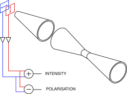
Figure 1: Schematic view of the Planck HFI polarisation dispositive using Polarisation Sensitive Bolometers.

With this design, the optical coupling to the sky should be identical for the two elements of the PSB (same beam shape, same response as a function of the wavelength), except for the sensitivity to orthogonal polarisation directions. Numerical simulations of the instrumental beam show that differences in beam shapes between the two polarisation directions of a single PSB are at negligible level (typically one per cent effect or less) Yurchenko (2001); Fosalba (2001). Noise levels, time constants of the detection chain (or more generally its impulse response), however, may differ slightly between the two elements, although at the manufacturing level it is hoped to match as well as possible the time constants and noise levels at the optimum (minimum) value.

The amount of depolarisation achieved with this design has been measured in-lab to be less than a few percent Maffei (2001), with a target of about 3 %, which should negligibly impact the sensitivity to polarised signals.

Each PSB, by differencing its two data streams, directly provides a measurement of the $Q$ Stokes parameter (i.e. a pure polarisation signal) in its own reference system (on an axis system where the $x$ and $y$ coordinates are measured along the two orthogonal polarisation-sensitive directions).

2.2 PSB layout

As emphasized in Couchot et al. (1999), at least three (linear) polarisation sensitive measurements with different orientations are needed to fully measure $I$, $Q$, and $U$ in a given direction. For perfectly matched, uncorrelated noise in the data, the minimal error box volume, as well as uncorrelated noise between the measurements of these three Stokes parameters, are realised when the polarimeter orientations are evenly distributed between 0 and 2$\pi$. Couchot et al. Couchot et al. (1999) denote such configurations (using $n\geq 3$ evenly distributed polarimeters) optimised configurations.

Then, a single PSB yielding two orthogonal polarisation measurements is not by itself sufficient to measure the three Stokes parameters $I$, $Q$, and $U$. The layout of the detectors for the Planck HFI is such that every PSB has a companion oriented at 45 degrees, with relative locations in the focal plane such that during scanning, it measures polarisation on the same pointing trajectory a fraction of a second before or after the first one (see Figure 2). Such a pair of companion PSBs yields four timelines which correspond effectively, after rephasing the measurements to get co-extensive pointings, to a polarisation measurement with a 4-polarimeter optimised configuration.

Figure 2: Polarisation measurement in the context of the Planck scan-strategy. For each PSB-pair detector set, the 4 measurements correspond to polarimeter orientations at 0, 45, 90 and 135 degrees with respect to the direction defined by the scanning.

Such a configuration has several advantages. The matching of the orientations with the scanning direction ensures that one of the PSBs permits (by simple difference) to measure $Q$ and the second $U$ in the reference system where one axis is parallel to the scanning and the other one perpendicular. The fact that two polarimeters share the same horn permits the best rejection of leakage of intensity $I$ signals into polarisation data, as discussed later. In addition, there is in principle built-in redundancy, as if even one detector fails, the three remaining timelines are sufficient to obtain the three Stokes parameters of interest (even if they do not then constitute an optimised configuration). This built-in redundancy permits an internal consistency check of the data (and thus of systematic effects) if all detectors work properly (in terms of sensitivity).

For each polarisation-sensitive frequency channel (at 143, 217 and 353 GHz), there are two such companion PSB pairs, which provides yet another redundancy level, as well as better overall sensitivity.

The HFI detector layout in the focal plane is shown in Figure 3.

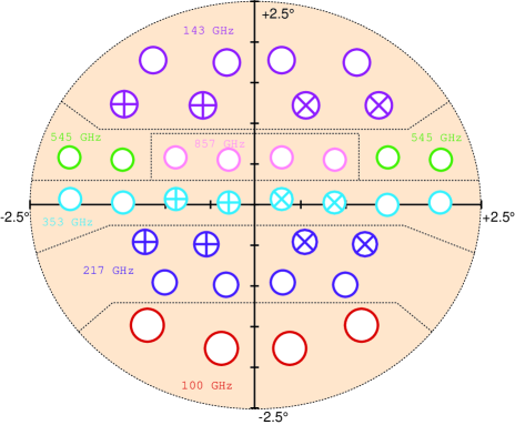
Figure 3: Planck HFI detector layout. In this figure, the horizontal and vertical axis are parallel and perpendicular to the line of scanning respectively. Polarisation bolometer fields of view are represented with a cross inside, showing the orientations of polarisation sensitivities.

3 Polarisation data processing

Whereas a lot of experience has been already gathered by the scientific community in the analysis of CMB anisotropy data, no such know-how has yet been acquired for the specific measurement of polarisation. Special effort has been undertaken in the HFI Data Processing Center (DPC) to develop data reduction tools specifically tailored and optimised for Planck HFI polarisation data. In this section, we discuss (non exhaustively) some of the issues adressed by the Planck HFI DPC so far, although part of the discussion applies (and we believe can be useful) to other instruments as well.

3.1 Modelling the measurement

There are several particularities to the measurement of polarisation, as compared to temperature, that will require the implementation of specific data processing software for the processing of such data. The specifics of polarisation signals come from two origins:

1. particularities of the signals we want to measure and which impact the data processing: very weak signals, poorly known galactic foregrounds and systematics;

2. specifics of the instrumental set-up for polarisation measurements.

Neglecting for the moment instrumental imperfections, each polarimeter of the Planck HFI, sensitive only to one linear polarisation, measures in each sample a linear combination of $I$, $Q$ and $U$ (integrated over the detector beam):

$$d(\alpha)=\frac{1}{2}\,[I+Q\cos 2\alpha+U\sin 2\alpha]$$ (1)

where $\alpha$ is the angle between the polarimeter orientation and the $x$-axis used for defining the Stokes parameters.

3.2 Combining data samples

At least three independent samples, with different angles $\alpha$ but coextensive beam pointings, are required to measure $I$, $Q$ and $U$. For an ideal measurement with two PSBs, assuming perfectly coincident beam pointings, the data from the four timelines are given by:

$$\left[\begin{array}[]{c}d_{1}\\ d_{2}\\ d_{3}\\ d_{4}\end{array}\right]=\left[\begin{array}[]{c}d(0)\\ d(\pi/2)\\ d(\pi/4)\\ d(3\pi/4)\end{array}\right]=\frac{1}{2}\left[\begin{array}[]{ccc}1&1&0\\ 1&-1&0\\ 1&0&1\\ 1&0&-1\end{array}\right]\left[\begin{array}[]{c}I\\ Q\\ U\end{array}\right]\,+\,\left[\begin{array}[]{c}n_{1}\\ n_{2}\\ n_{3}\\ n_{4}\end{array}\right]$$ (2)

where $n_{1},\ldots n_{4}$ are noise terms, and $I$, $Q$, $U$ denote the same beam-integrated Stokes parameters on the sky in the pointing direction. This equation can be recast in the matrix form:

$$d=AS+n$$ (3)

where $d$ is the data, $A$ a $4\times 3$ matrix, $S$ the three-element Stokes-parameter vector, and $n$ the noise.

With this ideal setup, for well balanced, uncorrelated noise, the best Stokes parameters estimates in the PSB-pair frame are obtained as

$$\begin{array}[]{ll}I&=\frac{1}{4}\times(d_{1}+d_{2}+d_{3}+d_{4})\\ Q&=\frac{1}{2}\times(d_{1}-d_{2})\\ U&=\frac{1}{2}\times(d_{3}-d_{4})\end{array}$$ (4)

For unbalanced and/or correlated noise, the optimal least square solution is

$$\widetilde{S}=[A^{t}N^{-1}A]^{-1}\,A^{t}N^{-1}d$$ (5)

where $N$ is the noise covariance matrix, $N_{ij}=\langle n_{i}n_{j}\rangle$.

3.3 Monitoring systematic effects

So far, we have not said anything about unavoidable noise correlations along the time streams, we have just considered the measurement at a single given pointing direction. In addition, all four detectors of a PSB pair have been assumed to have coextensive beams, which is actually not the case. The actual data processing for polarised map-making has to take into account these imperfections of the measurement. We concentrate on two major issues, which are low frequency drifts and pointing mismatch, and show how these imperfections impact polarised data processing for the Planck HFI.

3.3.1 Low frequency drifts

Low frequency drifts, due both to $1/f$ noise in the detection chain and to thermal fluctuations of payload elements detected by the sensors, are expected to be present in the detector timelines. This will be the case for PSB timelines as much as for unpolarised bolometers timelines. For each polarimeter $i$, writing explicitely the summmation over pixels to avoid confusion on other repeated indices, the data stream can be modelled as:

$$d_{it}=\sum_{p}M_{itp}[I_{p}+Q_{p}\cos 2\alpha_{itp}+U_{itp}\sin 2\alpha_{itp}]+n_{it}.$$ (6)

where $d_{it}$ is the data of polarimeter $i$ at time $t$, $(I_{p},Q_{p},U_{p})$ are the Stokes parameters in pixel $p$, $M_{itp}$ is the pointing matrix for polarimeter $i$, telling how much pixel $p$ contributes to the signal of polarimeter $i$ at time $t$. $\alpha_{itp}$ is the angle, in pixel $p$, between the co-polar direction of polarimeter $i$ at time $t$ and the reference direction (e.g. parallel and perpendicular to longitude and latitude lines), and $n_{it}$ is the noise timestream for detector $i$. Usually for temperature measurements, the pointing matrix is modelled as a sparse matrix containing only one non-vanishing element per line, which just tells which pixel of the sky is pointed at at time $t$.

Reordering the four timelines of a PSB pair $d_{it}$ into a single data vector $d$, the four noise streams into one single noise vector $n$, and the three maps of Stokes parameters $I_{p}$, $Q_{p}$ and $U_{p}$ into a single vector $S$, we can recast the four equations in eq. 6 (one for each detector) into one single linear equation:

$$d=MS+n.$$ (7)

Denoting as $N$ the noise autocorrelation (which now encompasses both correlations along timelines and correlations between timelines), the best estimates for the Stokes parameters, $\widetilde{S}$, can in principle be optained by a Global Least Square (GLS) inversion of the linear equation, $\widetilde{S}=[M^{t}N^{-1}M]^{-1}\,M^{t}N^{-1}d$. This however is a formidable task for Planck HFI, even for temperature maps, because of the size of the system. It is even more so with polarisation data.

A first-order map-making algorithm which approximates the GLS solution has been developped in Revenu et al. (2000) to construct polarisation maps from all timelines of an optimised configuration in the context of the Planck HFI. The method simplifies the resolution of the linear system under the assumption that noise correlations on timescales less than 60 seconds are negligible. Although a useful step towards a global solution, this simplified solution (which does not take into account imperfections of the model as it assumes a perfect knowledge of the pointing) can not be used for Planck in its present implementation. For polarisation mapping indeed, special care has to be taken in the implementation of the inversion of the linear system, as discussed in the next paragraphs.

3.3.2 Pointing mismatch

In the formal GLS solution, it is implicitly assumed that the matrix $M$, which encompasses both the pointing of the detectors and the mixing of the Stokes parameters, is known and perfectly describes the actual detector pointing. The fact that this is not exactly true complicates the processing of polarisation data in a somewhat tricky way.

Let us assume that a number $m$ of polarised data samples, all corresponding to a pointing towards the same given pixel $p$, are to be combined to recover a best estimate of $I$, $Q$ and $U$ at that point. For a pixel size $\theta_{p}$, the measurements are actually not pointing all to the exact same place, as illustrated in Figure 4. Any gradient of the temperature through the pixel will generate a difference in the readout of two polarimeters which do not integrate signal from perfectly co-extensive beams. For mismatched pointings, if the two polarimeters do not have the same orientation, a temperature gradient term will leak into the estimated polarisation (obtained through difference terms in the inversion of the linear system). This pointing error effect, even if essentially small or even negligible for temperature measurements, can nonetheless be important for polarisation because of the relative levels of $I$, $Q$ and $U$ on the sky.

For each pixel, the fake polarisation generated in this way will depend on the exact distribution of all pointings inside the pixel and on the distribution of corresponding polarimeter orientations. Relative pointings, therefore, are to be monitored very carefully for a polarisation-measuring experiment using single polarisers.

The naive model of the very sparse mixing matrix with one single non-vanishing element per line can be refined. The exact pointing, however, has to be perfectly well known, which is not the case in any of the present instruments (and not the case for Planck). The order of magnitude of the pointing reconstruction accuracy required for this effect to be smaller than the expected CMB polarisation for Planck is about 30 arcseconds. For the effect to be completely negligible, a relative pointing reconstruction of typically 5 arcseconds or better is needed. This requirement becomes less stringent in the limit of many measurements per pixel, as the effect of random uncorrelated errors in pointing reconstruction will tend to cancel out.

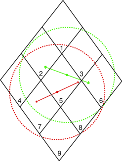
Figure 4: Illustration of the effect of single pixel pointing approximation or of pointing mismatch due to improper knowledge of the exact pointing. Here, in pixel 5, two polarisation measurements with different orientations are not pointed at the exact same place. Even if the beams are much bigger than the pixel, as should be for proper sampling, the difference between the two measurements includes a term proportional to the gradient of the beam-smoothed temperature map, which may be larger than the actual average polarisation in that pixel. For a careless implementation of a GLS map-making solution directly from polarimeter data streams, this may become a “killer–effect” for polarisation measurements.

3.3.3 Planck HFI polarised map-making

The use of Polarisation Sensitive Bolometers (or of any setup in which two orthogonal polarimeters share the same optics) provides an elegant solution to the pointing reconstruction accuracy problem, as beams are in principle perfectly co-extensive. Then, instead of implementing a GLS map-making on single polarimeter timelines, the map-making can be implemented on differences between two orthogonal polarimeter readouts. If the transfer functions of the two polarimeters in each PSB (time constants and readout impulse response) are well matched (which can be done by numerical post-filtering the two timelines if not built in hardware) the temperature gradient leakage problem is solved. This method is currently the baseline polarised map-making solution for nominal HFI performance (co-extensive PSB beams, nominal balanced noise levels, pointing reconstruction accuracies of a few tens of arcseconds or worse).

Additionnal discussion on polarisation systematics can be found in Kaplan & Delabrouille (2001).

3.3.4 Polarised component separation

Polarisation maps obtained with Planck in general, and the Planck HFI in particular, will contain at each frequency a mixture of the polarised emission of several astrophysical components. Although the component separation can be made based on the same general principles as for temperature maps, the overall performance of the separation is still unclear. First order methods assuming prior knowledge of the emission spectra and the spatial spectra have been developped Bouchet, Prunet & Sethi (1999) to generalise the Wiener separation method first implemented by Bouchet & Gispert Bouchet & Gispert (1999) and Tegmark & Efstathiou Tegmark & Efstathiou (1996). However, as little prior information on the polarised emission of foregrounds is actually available, blind separation methods Baccigalupi et al. (2000); Maino et al. (2001); Snoussi et al. (2001) must be investigated in this particular context.

Note still that for the Planck HFI, contrarily to the temperature case where several astrophysical foregrounds are expected to have temperature contribution larger than, or of the order of, the noise level, foreground polarised emission is expected to be well below both the polarisation sensitivity and the CMB polarisation, making component separation less critical for CMB polarisation measurements than for temperature anisotropies mapping (fig. 5).

4 The sensitivity of the Planck HFI

A detailed modelling of the performance of the HFI bolometers onboard Planck in the background conditions at the L2 Sun-Earth Lagrange point permits to predict the sensitivity of the HFI in each channel. For this estimation, it is assumed that the observation time is evenly shared between all the sky pixels. Corresponding estimated sensitivites on I, Q and U per resolution side square pixel, for all HFI frequency channels, are given in table 1.

The sensitivity of the Planck HFI to intensity and polarisation is shown in Figure 5. Galactic foreground emission level estimates are shown for high galactic latitudes ($b\simeq 70^{\circ}$). Sensitivity levels per resolution element ($1\sigma$) are shown as horizontal lines for six unpolarised frequency bands and three polarised frequency bands. The polarisation sensitivity is not sufficient to detect CMB polarisation at the level of individual pixels, nor to map foreground polarised emission at high galactic latitudes. Still, the power spectrum sensitivity on the 143 GHz channel alone (assuming the other channels are used as foreground and systematics monitors) is good enough to measure the $E-T$ and $E-E$ spectra quite well (Figure 6).

Most interestingly, the sensitivity of the Planck HFI is at a level which should allow to put strong contrains on $B$ modes, which are expected in a large range of cosmological scenarios to be much larger at low $\ell$ values than the $E$ modes of Figure 6, and thus within the detection reach of Planck (especially after combining the data from all HFI and LFI channels).

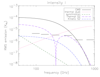
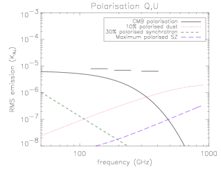
Figure 5: RMS intensity (left) and polarised emission (right) of various astrophysical components at high galactic latitude ($b\simeq 70^{\circ}$). Planck HFI Intensity and Polarisation sensitivities per resolution element in all frequency bands appear as horizontal bars on the plots.

Figure 6: HFI sensitivity to $E-T$ cross correlation (left) and to $E-E$ spectrum (right) for the 143 GHz HFI channel only. Power spectra are plotted for scalar modes only in a CDM-like cosmological model with $\Omega_{b}=0.045$, $H_{0}=65\,{\rm km/s/Mpc}$, $\Omega_{\Lambda}=0.7$ and $\Omega_{m}=0.3$, and have been obtained using the CMBFAST software Seljak & Zaldarriaga (1996).

5 Conclusion

Originally planned and proposed solely as a CMB temperature anisotropy sensitive instrument, the Planck HFI has been revised to become as well a CMB polarisation sensitive instrument. Unprecedented sensitivity at high resolution is achieved through the combination of the use of new polarisation sensitive bolometers, cooled to 100 mK on a spaceborne mission with low background, and of the selection of observing frequency bands where diffraction limits the resolution at the 5 to 7 arcminute level. In addition, the selected frequency range is at the expected minimum of the polarised emission from galactic foregrounds and extragalactic compact sources.

A substantial effort is being made to understand the impact of all possible systematic instrumental effects throughout the detection process and the data reduction pipeline. The minimisation of such systematic errors through a rigorous choice of the instrumental setup, careful on-ground testing, and continuing dedicated effort to the development and optimisation of data reduction methods for polarisation measurements with the Planck HFI, give us confidence that the instrument can meet its ambitious objectives.

6 Acknowledgements

We thank all the people who have contributed in a way or an other to the preparation of the measurement of polarisation with the Planck HFI. Special thanks to Yannick Giraud-Héraud, Jean-Michel Lamarre, Michel Piat, Cécile Renault and Cyrille Rosset for useful discussions and dedicated work. Thanks also to Jim Bartlett for useful suggestions towards improving the manuscript, and to Radek Stompor for interesting discussions about polarised map-making.

References

- Smoot et al. (1991) Smoot, G. F. et al., 1991, ApJ letter, 371, L1
- de Bernardis et al. (2000) de Bernardis, P. et al., 2000, Nature, 404, 955
- Lange et al. (2000) Lange, A. E. et al., 2001, Physical Review D, vol. 63, Issue 4, id. 042001
- Halverson et al. (2001) Halverson, N. W. et al., 2001, submitted to ApJ (astro-ph/0104489)
- Pryke et al. (2001) Pryke, C. et al., 2001, submitted to ApJ (astro-ph/0104490)
- Hanany et al. (2000) Hanany, S. et al., 2000, ApJ letter, 545, L5
- Lee et al. (2001) Lee, A. et al., 2001, ApJ letter, 561, L1
- Stompor et al. (2001) Stompor, R. et al., 2001, ApJ letter, 561, L7
- Jaffe et al. (2001) Jaffe, A. H. et al., 2001, Physical Review Letters, vol. 86, Issue 16, 3475
- Zaldarriaga & Seljak (1997) Zaldarriaga. M. & Seljak, U., 1997, Physical Review D, vol. 55, Issue 4, 1830
- Kamionkowski et al. (1997) Kamionkowski, M., Kosowsky, A. & Stebbins, A., 1997, Physical Review Letters, vol. 55, Issue 12, 7368
- Seljak & Zaldarriaga (1997) Seljak, U. & Zaldarriaga. M., 1997, Physical Review Letters, vol. 78, Issue 11, 2054
- Kamionkowski et al. (1997) Kamionkowski, M., Kosowsky, A. & Stebbins, A., 1997, Physical Review Letters, vol. 78, Issue 11, 2058
- Villa et al. (2001) Villa, F., on behalf of the Planck LFI, 2001, these proceedings.
- Bock et al. (2001) developped at Caltech/JPL by J. Bock and collaborators.
- Yurchenko (2001) Yurchenko, V., 2001, private communication
- Fosalba (2001) Fosabla, P., 2001, private communication
- Maffei (2001) Maffei., 2001, private communication
- Couchot et al. (1999) Couchot, F., Delabrouille, J., Kaplan, J., and Revenu, B., 1999, A&A Supplement Series, 135, 579
- Revenu et al. (2000) Revenu, B., Kim, A., Ansari, R., Couchot, F., Delabrouille, J., and J., K., 2000, A&A Supplement Series, 142, 499
- Kaplan & Delabrouille (2001) Kaplan, J. & Delabrouille, J., 2001, these proceedings.
- Bouchet & Gispert (1999) Bouchet, F.R., Gispert, R., 1999, NewA, 4, 443
- Tegmark & Efstathiou (1996) Tegmark, M. and Estathiou, G., 1996, MNRAS, 281, 1297
- Bouchet, Prunet & Sethi (1999) Bouchet, F.R., Prunet, S. and Sethi, Shiv K., 1999, MNRAS, 302, 663
- Baccigalupi et al. (2000) Baccigalupi, C. et al., 2000, MNRAS, 318, 769
- Maino et al. (2001) Maino, D. et al., 2001, submitted to MNRAS (astro-ph/0108362)
- Snoussi et al. (2001) Snoussi, H. et al., 2001, to appear in MaxEnt 2001 proceedings (astro-ph/0109123)
- Seljak & Zaldarriaga (1996) Seljak, U. & Zaldarriaga, M., 1996, ApJ 469, 437