Peculiar velocity effects in high-resolution microwave background experiments

Abstract

We investigate the impact of peculiar velocity effects due to the motion of the solar system relative to the microwave background (CMB) on high resolution CMB experiments. It is well known that on the largest angular scales the combined effects of Doppler shifts and aberration are important; the lowest Legendre multipoles of total intensity receive power from the large CMB monopole in transforming from the CMB frame. On small angular scales aberration dominates and is shown here to lead to significant distortions of the total intensity and polarization multipoles in transforming from the rest frame of the CMB to the frame of the solar system. We provide convenient analytic results for the distortions as series expansions in the relative velocity of the two frames, but at the highest resolutions a numerical quadrature is required. Although many of the high resolution multipoles themselves are severely distorted by the frame transformations, we show that their statistical properties distort by only an insignificant amount. Therefore, cosmological parameter estimation is insensitive to the transformation from the CMB frame (where theoretical predictions are calculated) to the rest frame of the experiment.

I Introduction

The impressive advances being made in sensitivity and resolution of microwave background (CMB) experiments demand that careful attention be paid to potential systematic effects in the analysis pipeline. Such effects can arise from imperfect modelling of the instrument, e.g. approximations in modelling the beam Challinor et al. (2000); Wu et al. (2001); Souradeep and Ratra (2001); Fosalba et al. (2001), or incomplete knowledge of the pointing, but also from more fundamental effects such as inaccurate separation of foregrounds (see e.g. Refs. Bouchet and Gispert (1999); Hobson et al. (1999) for reviews). In this paper we consider errors that may arise due to neglect of the peculiar motion of the experiment relative to the CMB rest frame (that frame in which the CMB dipole vanishes). For short duration experiments (e.g. balloon flights such as MAXIMA max and BOOMERANG boo ) the relative velocity is constant over the timescale of the experiment, but for experiments conducted over a few months or longer, and particularly for satellite surveys cob ; map ; pla , the variation in the relative velocity adds additional complications. In principle, the modulation of the aberration arising from any variation in the relative velocity must be accounted for with a more refined pointing model for the experiment van Leeuwen et al. (2001); Challinor et al. (2001) when making a map.

For a relative speed of $\beta c$ (where $c$ is the speed of light and $\beta\sim 1.23\times 10^{-3}$ for the solar-system barycenter relative to the CMB frame), the r.m.s. photon Doppler shifts and deflection angles are $\beta/\sqrt{3}$ and $\sqrt{2/3}\beta$ respectively. Despite these small values, significant distortions of the spherical multipoles of the total intensity and polarization fields do arise. A well known example is provided by the CMB dipole seen on earth, which, given the observed spectrum, arises from the transformation of the monopole in the CMB frame. More generally, on the largest angular scales the combined effects of Doppler shifts and aberration couple the total intensity monopole and dipole into the $l$th multipoles at the level $O(\beta^{l})$ and $O(\beta^{l-1})$ respectively. Given the size of the non-cosmological monopole, annual modulation of the dipole by the variation in the relative velocity of the earth in the CMB frame must be considered in long duration experiments.

In this paper we concentrate on the effects of peculiar velocities on small angular scale features in the microwave sky. On such scales, aberration dominates the distortions and becomes particularly acute when the angular scales of interest, $O(1/l)$, drop below the r.m.s. deflection angle, i.e. $l\gtrsim 800$ for the transformation from the CMB frame to that of the solar system. We provide simple analytic results for these distortions to the total intensity and polarization fields as power series in the relative velocity $\beta$. The power series converge rather slowly at the highest multipoles for most values of the azimuthal index $m$ [the leading-order corrections go like $O(l\beta)$] but the distortions can still easily be found semi-analytically with a one-dimensional quadrature. If the transformations of the multipoles carried through to their statistical properties, theoretical power spectra computed in linear theory (e.g. with standard Boltzmann codes Seljak and Zaldarriaga (1996); Lewis et al. (2000)) would not accurately describe the statistics of the high resolution multipoles observed on earth. (The theoretical power spectra would still be accurate in the CMB frame.) It is straightforward to calculate the statistical correlations of the multipoles observed on earth. Fortunately, as we show here, the statistical corrections due to peculiar velocity effects turn out to be negligible despite the large corrections to the individual multipoles. It follows that for the purposes of high resolution power spectrum and parameter estimation, the transformation from the CMB frame can be neglected.

This paper is arranged as follows. In Sec. II we describe the transformation laws for the total intensity multipoles in specific intensity and frequency-integrated forms. Convenient series expansions in $\beta$ of the transformations are provided, and their properties under rotations of the reference frames are described. The statistical poperties of the transformed multipoles are investigated by constructing rotationally-invariant power spectrum estimators and full correlation matrices. In Sec. III we discuss the geometry of the frame transformations for linear polarization, and present power series expansions for the transformations of the multipoles. The behaviour under rotations and parity are also outlined. Power spectra estimators and correlation matrices are constructed, and cross correlations with the total intensity are considered. Some implications of our results for survey missions are discussed in Sec. IV, which is followed by our conclusions in Sec. V. An appendix provides details of the evaluation of the multipole transformations as power series in $\beta$.

We use units with $c=1$.

II Transformation laws for total intensity

We consider the microwave sky as seen by two observers at the same event. Observer $S$ is equipped with a comoving tetrad $\{(e_{\mu})^{a}\}$, $\mu=\{0,1,2,3\}$, and observer $S^{\prime}$ carries the Lorentz-boosted tetrad $\{(e_{\mu}^{\prime})^{a}\}$. The relative velocity of $S^{\prime}$ as seen by $S$ has components on $\{(e_{i})^{a}\}$, $i=\{1,2,3\}$, which we denote by the spatial vector $\mathbf{v}$, which has magnitude $\beta$. The $S$ observer receives a photon with four-momentum $p^{a}$ when their line of sight is along $\hat{\mathbf{n}}$, so the photon propagation direction is $-\hat{\mathbf{n}}$. For $S$ the photon frequency is $\nu$ where $h\nu=p_{a}(e_{0})^{a}$ ($h$ is Planck’s constant), while $S^{\prime}$ observes frequency

$$\nu^{\prime}=\nu\gamma(1+\hat{\mathbf{n}}\cdot\mathbf{v}),$$ (1)

where $\gamma^{-2}=1-\beta^{2}$. The line of sight in $S^{\prime}$ is

$$\hat{\mathbf{n}}^{\prime}=\left(\frac{\hat{\mathbf{n}}\cdot\hat{\mathbf{v}}+\beta}{1+\hat{\mathbf{n}}\cdot\mathbf{v}}\right)\hat{\mathbf{v}}+\frac{\hat{\mathbf{n}}-\hat{\mathbf{n}}\cdot\hat{\mathbf{v}}\hat{\mathbf{v}}}{\gamma(1+\hat{\mathbf{n}}\cdot\mathbf{v})},$$ (2)

where $\hat{\mathbf{v}}$ is a unit vector in the direction of the relative velocity.

Denoting the sky brightness in total intensity seen by $S$ as $I(\nu,\hat{\mathbf{n}})$, the brightness seen by $S^{\prime}$ is (e.g. Ref. Misner et al. (1973))

$$I^{\prime}(\nu^{\prime},\hat{\mathbf{n}}^{\prime})=I(\nu,\hat{\mathbf{n}})\left(\frac{\nu^{\prime}}{\nu}\right)^{3}.$$ (3)

If $S$ and $S^{\prime}$ use their spatial triads $\{(e_{i})^{a}\}$ and $\{(e_{i}^{\prime})^{a}\}$ to define polar coordinates in the usual manner, and expand the sky brightness in terms of scalar spherical harmonics, i.e. $I(\nu,\hat{\mathbf{n}})=\sum_{lm}a_{lm}^{I}(\nu)Y_{lm}(\hat{\mathbf{n}})$, we find the following transformation law for the brightness multipoles:

$$a^{I\prime}_{lm}(\nu^{\prime})=\sum_{l^{\prime}m^{\prime}}\int\text{d}\hat{\mathbf{n}}\,\gamma(1+\hat{\mathbf{n}}\cdot\mathbf{v})a_{l^{\prime}m^{\prime}}^{I}(\nu)Y_{l^{\prime}m^{\prime}}(\hat{\mathbf{n}})Y_{lm}^{\ast}(\hat{\mathbf{n}}^{\prime}),$$ (4)

where $\nu=\nu^{\prime}\gamma^{-1}(1+\hat{\mathbf{n}}\cdot\mathbf{v})^{-1}$, and we have used $\nu^{\prime}{}^{2}\text{d}\hat{\mathbf{n}}^{\prime}=\nu^{2}\text{d}\hat{\mathbf{n}}$.

It will prove more convenient to consider the integral of the brightness over frequency, $I(\hat{\mathbf{n}})\equiv\int\text{d}\nu\,I(\nu,\hat{\mathbf{n}})$. The transformation law for this flux per solid angle follows from integrating Eq. (3):

$$I^{\prime}(\hat{\mathbf{n}}^{\prime})=I(\hat{\mathbf{n}})\left(\frac{\nu^{\prime}}{\nu}\right)^{4}.$$ (5)

Expanding $I(\hat{\mathbf{n}})$ in spherical harmonics, we find the multipole transformation law

$$a^{I\prime}_{lm} = \sum_{l^{\prime}m^{\prime}}a^{I}_{l^{\prime}m^{\prime}}\int\text{d}\hat{\mathbf{n}}\,[\gamma(1+\hat{\mathbf{n}}\cdot\mathbf{v})]^{2}Y_{l^{\prime}m^{\prime}}(\hat{\mathbf{n}})Y_{lm}^{\ast}(\hat{\mathbf{n}}^{\prime}),$$ (6)

$$= \sum_{l^{\prime}m^{\prime}}K_{(lm)(lm)^{\prime}}a^{I}_{l^{\prime}m^{\prime}}$$

where $a^{I}_{lm}=\int\text{d}\nu\,a^{I}_{lm}(\nu)$. The second equality defines the kernel $K_{(lm)(lm)^{\prime}}$ which relates the frequency-integrated multipoles in $S$ and $S^{\prime}$. Dividing $a^{I}_{lm}$ by four times the average flux per solid angle gives the multipoles of the gauge-invariant temperature anisotropy in linear theory (e.g. Refs. Stoeger et al. (1995); Maartens et al. (1995)).

If we choose the spacelike vectors of the tetrad $\{(e_{\mu})^{a}\}$ so that the relative velocity is along $(e_{3})^{a}$, the multipole transformation law becomes block-diagonal, $K_{(lm)(lm)^{\prime}}\propto\delta_{mm^{\prime}}$, with no coupling between different $m$ modes. The kernel for a general configuration can then be inferred from its transformation properties under rotations described in Sec. II.1. In the appendix we evaluate Eq. (4) as a series expansion in $\beta$ for general spin-weight functions, including terms up to $O(\beta^{2})$, for the case where $\mathbf{v}$ is aligned with $(e_{3})^{a}$. The expression is cumbersome, partly due to the fact that the transformation law is non-local in frequency. For large $l$ the aberration effect dominates Doppler shifts and the frequency spectrum of the multipoles is preserved by the transformation. We also give the result obtained by integrating over frequency; setting $s=0$ in Eq. (78) we find the series expansion of the kernel $K_{(lm)(lm)^{\prime}}$ up to $O(\beta^{2})$:

$$K_{(lm)(l^{\prime}m)} = \delta_{ll^{\prime}}\biggl{[}1+\frac{1}{2}\beta^{2}\biggl{(}C_{(l+1)m}^{2}(l-1)(l-2)+C_{lm}^{2}(l+2)(l+3)+m^{2}-l(l+1)+2\biggr{)}\biggr{]}$$ (7)

$$\mbox{}+\delta_{l(l^{\prime}+1)}\beta C_{lm}(l+3)-\delta_{l(l^{\prime}-1)}\beta C_{(l+1)m}(l-2)$$

$$\mbox{}+\delta_{l(l^{\prime}+2)}\beta^{2}C_{lm}C_{(l-1)m}\frac{1}{2}(l+2)(l+3)+\delta_{l(l^{\prime}-2)}\beta^{2}C_{(l+2)m}C_{(l+1)m}\frac{1}{2}(l-1)(l-2),$$

where $C_{lm}\equiv{}_{0}C_{lm}$ with

$${}_{s}C_{lm}\equiv\sqrt{\frac{(l^{2}-m^{2})(l^{2}-s^{2})}{l^{2}(4l^{2}-1)}}.$$ (8)

Comparison with Eq. (77) shows that for high $l$ the aberration effect described by the term $Y_{lm}^{\ast}(\hat{\mathbf{n}}^{\prime})$ in Eqs. (4) and (6) is dominant. For $\beta l\gtrsim 1$ the series is slow to converge for $|m|\ll l$ since the leading-order corrections go like $O(l\beta)$, reflecting the fact that the deflection angle due to aberration is comparable to the angular scale of the spherical harmonics at this $l$. For $\beta\approx 1.23\times 10^{-3}$, appropriate for the solar-system barycenter relative to the CMB frame, $\beta l\sim 1$ corresponds to multipoles $l\sim 800$. In this case, the kernel $K_{(lm)(lm)^{\prime}}$ is easily evaluated by a numerical quadrature. We show some representative elements of the kernel in Fig. 1, which demonstrates that the multipoles do indeed suffer severe distortion for $l\gtrsim 1/\beta$, as suggested by Eq. (7). For $|m|$ close to $l$, ${}_{s}C_{lm}\sim O(l^{-1/2})$ and retaining only the terms given in Eq. (7) is accurate to much better than 0.1 per cent for the $l$ range probed by e.g. Planck ($l\lesssim 2000$). For such values of $m$ the distortions to the multipoles are only small, with leading-order corrections at $l^{\prime}=l\pm 1$ of $O(\beta\sqrt{l})$. For $l\beta\ll 1$, the departures of the kernel from the identity $\delta_{ll^{\prime}}\delta_{mm^{\prime}}$ are very small, giving negligible distortions to the multipoles except for $l$ close to unity when the non-zero coupling to the (large) monopole can give significant distortions, as described in Sec. I.

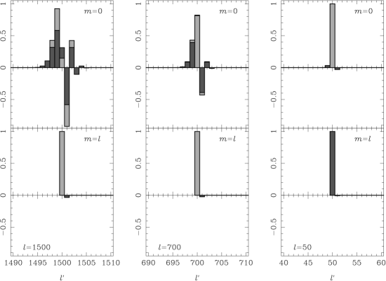
Figure 1: Representative elements of the frequency-integrated kernel $K_{(lm)(lm)^{\prime}}$ evaluated with the relative velocity ($\beta=1.23\times 10^{-3}$) along $(e_{3})^{a}$. The results of a numerical integration of Eq. (6) are shown in dark gray, while results based on the series expansion (7) are shown in light gray. The smaller (absolute values) of the two are shown in the foreground. Elements are shown for $l=1500$ (left), $l=700$ (middle), and $l=50$ (right), with $m=0$ (top) and $m=l$ (bottom).

II.1 Rotational properties

If we rotate the relative velocity $\mathbf{v}$ to $D\mathbf{v}$ keeping the tetrad $(e_{\mu})^{a}$ fixed, [thus inducing a transformation of the Lorentz-boosted tetrad $(e_{\mu}^{\prime})^{a}$], the frequency-integrated multipoles continue to be given by Eq. (6), but with $\mathbf{v}$ replaced by $D\mathbf{v}$ in $\hat{\mathbf{n}}^{\prime}$ [Eq. (2)] and in $(1+\hat{\mathbf{n}}\cdot\mathbf{v})$. With the change of integration variable $\hat{\mathbf{n}}\rightarrow D\hat{\mathbf{n}}$, the integral defining the transformed kernel $K_{(lm)(lm)^{\prime}}(D\mathbf{v})$ becomes

$$\int\text{d}\hat{\mathbf{n}}\,\gamma^{2}(1+\hat{\mathbf{n}}\cdot\mathbf{v})Y_{l^{\prime}m^{\prime}}(D\hat{\mathbf{n}})Y_{lm}^{\ast}(D\hat{\mathbf{n}}^{\prime})=\int\text{d}\hat{\mathbf{n}}\,\gamma^{2}(1+\hat{\mathbf{n}}\cdot\mathbf{v})D^{-1}Y_{l^{\prime}m^{\prime}}(\hat{\mathbf{n}})[D^{-1}Y_{lm}(\hat{\mathbf{n}}^{\prime})]^{\ast},$$ (9)

where $D^{-1}Y_{l^{\prime}m^{\prime}}(\hat{\mathbf{n}})=\sum_{m^{\prime\prime}}D^{l\ast}_{m^{\prime}m^{\prime\prime}}Y_{lm^{\prime\prime}}(\hat{\mathbf{n}})$ with $D^{l}_{mm^{\prime}}$ a Wigner $D$-matrix. (Our conventions for $D$-matrices follow Refs. Brink and Satchler (1993); Varshalovich et al. (1988).) It follows that the transformed kernel is given by

$$K_{(lm)(lm)^{\prime}}(D\mathbf{v})=\sum_{MM^{\prime}}D^{l}_{mM}{}K_{(lM)(lM)^{\prime}}(\mathbf{v})D^{l^{\prime}\ast}_{m^{\prime}M^{\prime}}.$$ (10)

Instead of rotating the (physical) relative velocity of $S$ and $S^{\prime}$, we could imagine rotating the spatial triad $(e_{i})^{a}\rightarrow D(e_{i})^{a}$. Under this coordinate transformation, the Lorentz-boosted frame vectors transform similarly: $(e^{\prime}_{i})^{a}\rightarrow D(e^{\prime}_{i})^{a}$. For a fixed sky, the multipoles seen by $S$ and $S^{\prime}$ transform according to e.g. $a^{I}_{lm}\rightarrow\sum_{m^{\prime}}D^{l\ast}_{m^{\prime}m}a^{I}_{lm^{\prime}}$ (which is equivalent to rotating the sky with $D^{-1}$ leaving the tetrad fixed). It follows that under coordinate rotations, the kernel transforms as

$$K_{(lm)(lm)^{\prime}}\rightarrow D^{l\ast}_{Mm}K_{(lM)(lM)^{\prime}}D^{l^{\prime}}_{M^{\prime}m^{\prime}}.$$ (11)

Note that the (passive) rotation of the frame vectors by $D^{-1}$ has the same effect on the kernel as the (active) rotation of the relative velocity $\mathbf{v}$ by $D$, as expected.

Finally, we consider (active) parity transformations $\mathbf{v}\rightarrow-\mathbf{v}$ with the tetrad $(e_{\mu})^{a}$ held fixed. Using $Y_{lm}(-\hat{\mathbf{n}})=(-1)^{l}Y_{lm}(\hat{\mathbf{n}})$ it is straightforward to show that

$$K_{(lm)(lm)^{\prime}}(-\mathbf{v})=(-1)^{l+l^{\prime}}K_{(lm)(lm)^{\prime}}(\mathbf{v}).$$ (12)

The behaviour of the kernel under parity ensures that if we simultaneously invert $\mathbf{v}$ and the sky [$a^{I}_{lm}\rightarrow(-1)^{l}a^{I}_{lm}$], the multipoles seen by $S^{\prime}$ transform to $(-1)^{l}a^{I\prime}_{lm}$.

These transformation properties of the kernel under rotations allow one to generalise Eq. (7) easily to the case where $\mathbf{v}$ is not aligned with $(e_{3})^{a}$.

II.2 Power spectrum estimators

We have seen how aberration effects lead to significant distortions of some of the high-$l$ multipoles in transforming from the CMB frame to the frame of the experiment. In the next two subsections we investigate the impact of these distortions on the statistical properties of the multipoles.

We assume that in the CMB frame ($S$) the second-order statistics of the anisotropies are summarised by

$$\langle a^{I}_{lm}a^{I\ast}_{l^{\prime}m^{\prime}}\rangle=C^{II}_{l}\delta_{ll^{\prime}}\delta_{mm^{\prime}},$$ (13)

appropriate to a statistically-isotropic ensemble with power spectrum $C^{II}_{l}$. (The averaging is over an ensemble of CMB realizations.) It is this $C_{l}$ for $l\geq 2$ that is computed with linear perturbation theory in standard Boltzmann codes (e.g. Refs. Seljak and Zaldarriaga (1996); Lewis et al. (2000)).

We begin by considering the quadratic statistic

$$\hat{C}^{II\prime}_{l}\equiv\frac{1}{2l+1}\sum_{m}|a^{I\prime}_{lm}|^{2},$$ (14)

which is evaluated by $S^{\prime}$. In the absence of noise this statistic is the optimal (minimum-variance) estimator for the power spectrum if we ignore peculiar velocity effects. By construction, $\hat{C}^{II\prime}_{l}$ is independent of the choice of spatial triad, but is only invariant under rotations of the sky in $S$ ($a^{I}_{lm}\rightarrow D^{l}_{mm^{\prime}}a_{lm^{\prime}}^{I}$) if the relative velocity is also rotated to $D\mathbf{v}$. However, averaging over CMB realizations keeping the relative velocity fixed we obtain a quantity $\langle\hat{C}^{II\prime}_{l}\rangle$ which is obviously invariant under rotations of the sky in $S$. The average $\langle\hat{C}^{II\prime}_{l}\rangle$, which determines the bias of the power spectrum estimator $\hat{C}^{II\prime}_{l}$, is linearly related to the $C^{II}_{l}$:

$$\langle\hat{C}^{II\prime}_{l}\rangle = \frac{1}{2l+1}\sum_{l^{\prime}mm^{\prime}}|K_{(lm)(lm)^{\prime}}|^{2}C^{II}_{l^{\prime}}$$ (15)

$$\equiv \sum_{l^{\prime}}W_{ll^{\prime}}C^{II}_{l^{\prime}}.$$

The kernel $W_{ll^{\prime}}$ depends only on the relative speed $\beta$ and not the direction $\hat{\mathbf{v}}$, so we can always evaluate it with $\mathbf{v}$ aligned with $(e_{3})^{a}$.

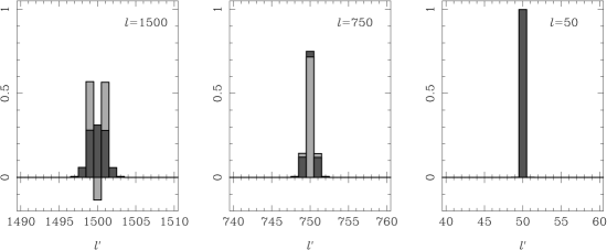
Figure 2: Representative elements of the kernel $W_{ll^{\prime}}$ evaluated with relative velocity $\beta=1.23\times 10^{-3}$. The results of a numerical integration of are shown in dark gray, while results based on the series expansion (16) are shown in light gray. The smaller (absolute values) of the two are shown in the foreground. Elements are shown for $l=1500$ (left), $l=700$ (middle), and $l=50$ (right).

The series expansion (7) of $K_{(lm)(lm^{\prime})}$ can be used to evaluate $W_{ll^{\prime}}$. Correct to $O(\beta^{2})$ we find

$$W_{ll^{\prime}}=\delta_{ll^{\prime}}\left(1-\frac{1}{3}\beta^{2}(l^{2}+l-8)\right)+\delta_{l(l^{\prime}+1)}\beta^{2}\frac{l(l+3)^{2}}{3(2l+1)}+\delta_{l(l^{\prime}-1)}\beta^{2}\frac{(l-2)^{2}(l+1)}{3(2l+1)}.$$ (16)

Again the series is slow to converge for $l\beta\gtrsim 1$ and the terms neglected in Eq. (16) are non-negligible. We show $W_{ll^{\prime}}$ for some representative $l$ values in Fig. 2. It is clear from the figure that $W_{ll^{\prime}}$ is well localised in comparison to any features in the CMB power spectrum for the range of $\beta$ of interest here. In this case, we can approximate

$$\langle\hat{C}^{II^{\prime}}_{l}\rangle \approx C^{II}_{l}\sum_{l^{\prime}}W_{ll^{\prime}}$$ (17)

$$= C^{II}_{l}[1+4\beta^{2}+O(\beta^{3})].$$

The effect of the velocity transformation is thus to rescale the amplitude of the power spectrum by $1+4\beta^{2}$. This bias is clearly insignificant. $\sum_{l^{\prime}}W_{ll^{\prime}}$ is actually independent of $l$ to all orders in $\beta$. To see this we form $\sum_{l^{\prime}}W_{ll^{\prime}}$ directly using the integral expression (6) for $K_{(lm)(lm)^{\prime}}$. The result simplifies to

$$\sum_{l^{\prime}}W_{ll^{\prime}}=\frac{\gamma^{4}}{4\pi}\int\text{d}\hat{\mathbf{n}}\,(1+\hat{\mathbf{n}}\cdot\mathbf{v})^{4}=\gamma^{4}\left(1+2\beta^{2}+\frac{1}{5}\beta^{4}\right),$$ (18)

on using the completeness relation

$$\sum_{lm}{}_{s}Y_{lm}(\hat{\mathbf{n}}_{1}){}_{s}Y_{lm}^{\ast}(\hat{\mathbf{n}}_{2})=\delta(\hat{\mathbf{n}}_{1}-\hat{\mathbf{n}}_{2}),$$ (19)

and the addition theorem for the spherical harmonics. The series expansion of Eq. (18) agrees with Eq. (17). We conclude that despite the fact that the multipoles themselves can be severely distorted by aberration for $l\beta\gtrsim 1$ in passing from the CMB frame to that of the solar system, the quadratic power spectrum estimator is negligibly biased since the effect of the velocity transformation is to convolve the power spectrum with a narrow kernel $W_{ll^{\prime}}$ that sums to very nearly unity.

II.3 Signal covariance matrix

Assuming Gaussian statistics in the CMB frame, the multipoles $a^{I\prime}_{lm}$ in $S^{\prime}$ will also be distributed according to a multivariate Gaussian since the transformation (6) is linear. In this case, the covariance matrix $\langle a^{I\prime}_{lm}a^{I\prime\ast}_{l^{\prime}m^{\prime}}\rangle$ contains all statistical information about the anisotropies in $S^{\prime}$, and as such is an essential element of optimal power spectrum estimation.

If we make use of Eq. (13), the covariance matrix in $S^{\prime}$ reduces to

$$\langle a^{I\prime}_{lm}a^{I\prime\ast}_{l^{\prime}m^{\prime}}\rangle=\sum_{LM}K_{(lm)(LM)}K^{\ast}_{(lm)^{\prime}(LM)}C_{L}^{II}.$$ (20)

The presence of the preferred direction $\hat{\mathbf{v}}$ breaks statistical isotropy in $S^{\prime}$, and the multipoles are correlated for $l\neq l^{\prime}$ and $m\neq m^{\prime}$. The structure of the covariance matrix in $S^{\prime}$ depends on the choice of the spatial triad $(e_{i})^{a}$ with respect to the relative velocity of the two observers. Aligning $(e_{3})^{a}$ with $\mathbf{v}$, the $m$-modes decouple in $K_{(lm)(lm)^{\prime}}$ and so also in the covariance matrix. Furthermore, for the values of $\beta$ of interest here ($\beta\ll 1$), the kernel $K_{(lm)(lm)^{\prime}}$ falls rapidly to zero for $l$ and $l^{\prime}$ differing by more than a few (see Fig. 1), so the same will be true of the covariance matrix. It follows that we can approximate

$$\langle a^{I\prime}_{lm}a^{I\prime\ast}_{l^{\prime}m^{\prime}}\rangle\approx C^{II}_{l}\sum_{LM}K_{(lm)(LM)}K^{\ast}_{(lm)^{\prime}(LM)}.$$ (21)

(Pulling out $C^{II}_{l^{\prime}}$ instead will give essentially the same result for smooth power spectra.) The summation in Eq. (21) is most easily evaluated by substituting the integral representation (6) for $K_{(lm)(LM)}$ and using the completeness relation (19). We find that $\sum_{LM}K_{(lm)(LM)}K^{\ast}_{(lm)^{\prime}(LM)}$ reduces to the integral

$$\int\text{d}\hat{\mathbf{n}}\,[\gamma(1+\hat{\mathbf{n}}\cdot\mathbf{v})]^{4}Y_{lm}^{\ast}(\hat{\mathbf{n}}^{\prime})Y_{l^{\prime}m^{\prime}}(\hat{\mathbf{n}}^{\prime})=\int\text{d}\hat{\mathbf{n}}^{\prime}\,[\gamma(1-\hat{\mathbf{n}}^{\prime}\cdot\mathbf{v})]^{-6}Y_{lm}^{\ast}(\hat{\mathbf{n}}^{\prime})Y_{l^{\prime}m^{\prime}}(\hat{\mathbf{n}}^{\prime}),$$ (22)

where we changed the integration variable to $\hat{\mathbf{n}}^{\prime}$ and used $\gamma(1+\hat{\mathbf{n}}\cdot\mathbf{v})=[\gamma(1-\hat{\mathbf{n}}^{\prime}\cdot\mathbf{v})]^{-1}$. Note that both spherical harmonics have the same argument in the integrand, so we don’t expect the same $O(l\beta)$ terms at high $l$ that arise in the kernel $K_{(lm)(lm)^{\prime}}$. Eq. (22) can easily be evaluated for $(e_{3})^{a}$ along $\mathbf{v}$ (in which case there is no coupling between different $m$) by expanding in $\beta$:

$$\sum_{LM}K_{(lm)(LM)}K^{\ast}_{(l^{\prime}m)(LM)} = \delta_{ll^{\prime}}[1+3\beta^{2}(7C_{(l+1)m}^{2}+7C_{lm}^{2}-1)]+\delta_{l(l^{\prime}+1)}6\beta C_{lm}+\delta_{l(l^{\prime}-1)}6\beta C_{(l+1)m}$$ (23)

$$\mbox{}+\delta_{l(l^{\prime}+2)}21\beta^{2}C_{lm}C_{(l-1)m}+\delta_{l(l^{\prime}-2)}21\beta^{2}C_{(l+2)m}C_{(l+1)m}+O(\beta^{3}).$$

This result for the covariance matrix in $S^{\prime}$ could easily be used in maximum-likelihood power spectrum estimation (see e.g. Ref. Bond et al. (1998)) to correct for the bias due to peculiar velocity effects. However, since the leading corrections are only $O(\beta)$, even at high $l$, the effects will be negligible.

III Transformation laws for linear polarization

The linearly polarized brightness in $S$ is described by Stokes parameters $Q(\nu,\hat{\mathbf{n}})$ and $U(\nu,\hat{\mathbf{n}})$. The Stokes parameters depend on a specific choice of orthonormal basis vectors $\{\mathbf{m}_{1},\mathbf{m}_{2}\}$ for each line of sight $\hat{\mathbf{n}}$. If $\{\mathbf{m}_{1},\mathbf{m}_{2},-\hat{\mathbf{n}}\}$ form a right-handed orthonormal set, the Stokes parameters are related to the linear polarization tensor by

$${\mathcal{P}}^{ab}=\frac{1}{2}[Q(\mathbf{m}_{1}\otimes\mathbf{m}_{1}-\mathbf{m}_{2}\otimes\mathbf{m}_{2})+U(\mathbf{m}_{1}\otimes\mathbf{m}_{2}+\mathbf{m}_{2}\otimes\mathbf{m}_{1})].$$ (24)

The Stokes parameters transform under changes of frame in the same way as the total intensity, i.e.

$$Q^{\prime}(\nu^{\prime},\hat{\mathbf{n}}^{\prime})=Q(\nu,\hat{\mathbf{n}})\left(\frac{\nu^{\prime}}{\nu}\right)^{3},$$ (25)

and similarly for $U$, provided that the basis vectors are transformed according to Challinor (2000)

$$\mathbf{m}^{\prime}_{i}=\mathbf{m}_{i}+(\gamma-1)\mathbf{m}_{i}\cdot\hat{\mathbf{v}}\hat{\mathbf{v}}-\gamma\mathbf{m}_{i}\cdot\mathbf{v}\hat{\mathbf{n}}^{\prime},$$ (26)

where $i=1,2$. It is straightforward to verify that this transformation law preserves orthonormality, and also that $\mathbf{m}^{\prime}_{i}$ is obtained from $\mathbf{m}_{i}$ by parallel transport on the unit sphere along the great circle through $\hat{\mathbf{n}}$ and $\hat{\mathbf{n}}^{\prime}$ (and so through $\hat{\mathbf{v}}$ also). In terms of the polarization tensor, the frame transformation law can be written as

$${\mathcal{P}}^{\prime ab}(\nu^{\prime},\hat{\mathbf{n}}^{\prime})={\mathcal{P}}^{ab}_{\|}(\nu,\hat{\mathbf{n}};\mathbf{v})\left(\frac{\nu^{\prime}}{\nu}\right)^{3},$$ (27)

where ${\mathcal{P}}^{ab}_{\|}(\nu,\hat{\mathbf{n}};\mathbf{v})$ is ${\mathcal{P}}^{ab}(\nu,\hat{\mathbf{n}})$ parallel propagated to $\hat{\mathbf{n}}^{\prime}$. The 1+3 covariant form of this transformation was given in Ref. Challinor (2000).

If $S$ and $S^{\prime}$ introduce polar coordinates as in Sec. II, the polarization tensor can be expanded in symmetric trace-free tensor harmonics Kamionkowski et al. (1997a):

$${\mathcal{P}}_{ab}(\nu,\hat{\mathbf{n}})=\frac{1}{\sqrt{2}}\sum_{lm}a^{E}_{lm}(\nu)Y^{G}_{(lm)ab}(\hat{\mathbf{n}})+a^{B}_{lm}(\nu)Y^{C}_{(lm)ab}(\hat{\mathbf{n}}),$$ (28)

which defines the electric ($E$) and magnetic ($B$) multipoles. Using Eq. (27) we can extract the multipoles seen by $S^{\prime}$. For $a^{E\prime}_{lm}(\nu^{\prime})$ we find

$$a^{E\prime}_{lm}(\nu^{\prime})=\sum_{l^{\prime}m^{\prime}}\int\text{d}\hat{\mathbf{n}}\,\gamma(1+\hat{\mathbf{n}}\cdot\mathbf{v})[a^{E}_{l^{\prime}m^{\prime}}(\nu^{\prime})Y^{G\,ab}_{\|(lm)^{\prime}}(\hat{\mathbf{n}};\mathbf{v})Y^{G\ast}_{(lm)ab}(\hat{\mathbf{n}}^{\prime})+a^{B}_{l^{\prime}m^{\prime}}(\nu^{\prime})Y^{C\,ab}_{\|(lm)^{\prime}}(\hat{\mathbf{n}};\mathbf{v})Y^{G\ast}_{(lm)ab}(\hat{\mathbf{n}}^{\prime})],$$ (29)

with a similar result for $a^{B\prime}_{lm}(\nu^{\prime})$. Here $Y^{G\,ab}_{\|(lm)}(\hat{\mathbf{n}};\mathbf{v})$ is $Y^{G\,ab}_{(lm)}(\hat{\mathbf{n}})$ parallel propagated to $\hat{\mathbf{n}}^{\prime}$, and similarly for the curl harmonics. Note how in general the frame transformation mixes $E$ and $B$ polarization. Equation (29) is valid quite generally, and is useful for discussing the rotational properties of the transformations (see later). However, to compute the transformation laws it is again convenient to arrange $(e_{i})^{a}$ so that $\mathbf{v}$ is along $(e_{3})^{a}$. We can then exploit the fact that the polar basis vector fields $\hat{\bm{\theta}}(\hat{\mathbf{n}})$ and $\hat{\bm{\phi}}(\hat{\mathbf{n}})$ are parallel propagated along longitudes to simplify $Y^{G\,ab}_{\|(lm)}(\hat{\mathbf{n}};\mathbf{v})$. The gradient and curl harmonics can be written in terms of spin-weight $\pm 2$ harmonics (our conventions follow Refs. Ng and Liu (1999); Challinor et al. (2000)):

$$Y^{G\,ab}_{lm} = \frac{1}{\sqrt{2}}({}_{-2}Y_{lm}\mathbf{m}\otimes\mathbf{m}+{}_{2}Y_{lm}\mathbf{m}^{\ast}\otimes\mathbf{m}^{\ast}),$$ (30)

$$Y^{C\,ab}_{lm} = \frac{1}{i\sqrt{2}}({}_{-2}Y_{lm}\mathbf{m}\otimes\mathbf{m}-{}_{2}Y_{lm}\mathbf{m}^{\ast}\otimes\mathbf{m}^{\ast}),$$ (31)

where the complex vector $\mathbf{m}\equiv(\hat{\bm{\theta}}+i\hat{\bm{\phi}})/\sqrt{2}$, so that Eq. (29) can be written as

$$(a^{E\prime}_{lm}\pm ia^{B\prime}_{lm})(\nu^{\prime})=\sum_{l^{\prime}m^{\prime}}(a^{E}_{l^{\prime}m^{\prime}}\pm ia^{B}_{l^{\prime}m^{\prime}})(\nu)\int\text{d}\hat{\mathbf{n}}\,\gamma(1+\hat{\mathbf{n}}\cdot\mathbf{v}){}_{\pm 2}Y_{l^{\prime}m^{\prime}}(\hat{\mathbf{n}}){}_{\pm 2}Y_{lm}^{\ast}(\hat{\mathbf{n}}^{\prime}).$$ (32)

The integral on the right-hand side is evaluated as a power series in $\beta$ for general spin-weight $s$ in the appendix.

For our purposes it will be more convenient to consider the frequency-integrated multipoles, e.g. $a^{E}_{lm}=\int\text{d}\nu\,a^{E}_{lm}(\nu)$. Integrating Eq. (29) over frequency, we find

$$a^{E\prime}_{lm} = \sum_{l^{\prime}m^{\prime}}{}_{+}K_{(lm)(lm)^{\prime}}a^{E}_{l^{\prime}m^{\prime}}+i{}_{-}K_{(lm)(lm)^{\prime}}a^{B}_{l^{\prime}m^{\prime}},$$ (33)

$$a^{B\prime}_{lm} = \sum_{l^{\prime}m^{\prime}}{}_{+}K_{(lm)(lm)^{\prime}}a^{B}_{l^{\prime}m^{\prime}}-i{}_{-}K_{(lm)(lm)^{\prime}}a^{E}_{l^{\prime}m^{\prime}},$$ (34)

where the kernels

$${}_{+}K_{(lm)(lm)^{\prime}} = \int\text{d}\hat{\mathbf{n}}\,[\gamma(1+\hat{\mathbf{n}}\cdot\mathbf{v})]^{2}Y^{G\,ab}_{\|(lm)^{\prime}}(\hat{\mathbf{n}};\mathbf{v})Y^{G\ast}_{(lm)ab}(\hat{\mathbf{n}}^{\prime})=\int\text{d}\hat{\mathbf{n}}\,[\gamma(1+\hat{\mathbf{n}}\cdot\mathbf{v})]^{2}Y^{C\,ab}_{\|(lm)^{\prime}}(\hat{\mathbf{n}};\mathbf{v})Y^{C\ast}_{(lm)ab}(\hat{\mathbf{n}}^{\prime}),$$ (35)

$${}_{-}K_{(lm)(lm)^{\prime}} = -i\int\text{d}\hat{\mathbf{n}}\,[\gamma(1+\hat{\mathbf{n}}\cdot\mathbf{v})]^{2}Y^{C\,ab}_{\|(lm)^{\prime}}(\hat{\mathbf{n}};\mathbf{v})Y^{G\ast}_{(lm)ab}(\hat{\mathbf{n}}^{\prime})=i\int\text{d}\hat{\mathbf{n}}\,[\gamma(1+\hat{\mathbf{n}}\cdot\mathbf{v})]^{2}Y^{G\,ab}_{\|(lm)^{\prime}}(\hat{\mathbf{n}};\mathbf{v})Y^{C\ast}_{(lm)ab}(\hat{\mathbf{n}}^{\prime}).$$ (36)

The behaviour of ${}_{\pm}K_{(lm)(lm)^{\prime}}$ under rotations $\mathbf{v}\rightarrow D\mathbf{v}$ is the same as for the total intensity kernel, Eq. (10), since the tensor harmonics transform under rigid rotations with the same $D$-matrices as the scalar harmonics Challinor et al. (2000). This property of the tensor harmonics also ensures that under rotations of the coordinate system, $(e_{i})^{a}\rightarrow D(e_{i})^{a}$, the electric and magnetic multipoles transform irreducibly to e.g. $\sum_{m^{\prime}}D^{l\ast}_{m^{\prime}m}{}a^{E}_{lm^{\prime}}$. Under inversion of $\mathbf{v}$ with $(e_{\mu})^{a}$ held fixed, the kernels transform to

$${}_{+}K_{(lm)(lm)^{\prime}}(-\mathbf{v}) = (-1)^{l+l^{\prime}}{}_{+}K_{(lm)(lm)^{\prime}}(\mathbf{v}),$$ (37)

$${}_{-}K_{(lm)(lm)^{\prime}}(-\mathbf{v}) = -(-1)^{l+l^{\prime}}{}_{-}K_{(lm)(lm)^{\prime}}(\mathbf{v}),$$ (38)

so that under simultaneous inversion of the sky in $S$, $a^{E}_{lm}\rightarrow(-1)^{l}a^{E}_{lm}$ and $a^{B}_{lm}\rightarrow(-1)^{l+1}a^{B}_{lm}$, and inversion of $\mathbf{v}$, the multipoles in $S^{\prime}$ transform like those in $S$.

The frequency-integrated kernels are most simply evaluated with $\mathbf{v}$ along $(e_{3})^{a}$. In this case the $m$-modes decouple, as with the total intensity. Writing ${}_{\pm}K=({}_{2}K\pm{}_{-2}K)/2$, we can use Eq. (78), which evaluates ${}_{s}K_{(lm)(lm)^{\prime}}$ as a series correct to $O(\beta^{2})$, to show that

$${}_{+}K_{(lm)(l^{\prime}m)} = \delta_{ll^{\prime}}\biggl{[}1+\frac{1}{2}\beta^{2}\biggl{(}{}_{2}C_{(l+1)m}^{2}(l-1)(l-2)+{}_{2}C_{lm}^{2}(l+2)(l+3)+m^{2}-l(l+1)+6-\frac{4m^{2}}{l(l+1)}+\frac{24m^{2}}{l^{2}(l+1)^{2}}\biggr{)}\biggr{]}$$ (39)

$$+ \delta_{l(l^{\prime}+1)}\beta{}_{2}C_{lm}(l+3)-\delta_{l(l^{\prime}-1)}\beta{}_{2}C_{(l+1)m}(l-2)$$

$$+ \delta_{l(l^{\prime}+2)}\beta^{2}{}_{2}C_{lm}{}_{2}C_{(l-1)m}\frac{1}{2}(l+2)(l+3)+\delta_{l(l^{\prime}-2)}\beta^{2}{}_{2}C_{(l+2)m}{}_{2}C_{(l+1)m}\frac{1}{2}(l-1)(l-2),$$

and

$${}_{-}K_{(lm)(l^{\prime}m)}=-\delta_{ll^{\prime}}\frac{6\beta m}{l(l+1)}-\delta_{l(l^{\prime}+1)}{}_{2}C_{lm}(l+3)\frac{6\beta^{2}m}{(l+1)(l-1)}+\delta_{l(l^{\prime}-1)}{}_{2}C_{(l+1)m}(l-2)\frac{6\beta^{2}m}{l(l+2)}.$$ (40)

(Equivalent results, correct to $O(\beta)$, have already been worked out in 1+3 covariant form Challinor (2000).) The kernel ${}_{-}K_{(lm)(lm)^{\prime}}$ is suppressed at high $l$. It receives comparable contributions from Doppler and aberration effects for all $l$ [see Eq. (77)] in contrast to the ${}_{+}K_{(lm)(lm)^{\prime}}$ and the total intensity kernel $K_{(lm)(lm)^{\prime}}$ which are dominated by aberration effects at high $l$. The series expansion of ${}_{+}K_{(lm)(lm)^{\prime}}$ is slow to converge for $l\beta\gtrsim 1$ when $|m|\ll l$, and there are large distortions to the electric and magnetic multipoles for these indices. Electric multipoles nearby in $l$ couple in strongly to distort $a^{E}_{lm}$, and similarly for the magnetic multipoles. For $l\gg 1$ the kernel ${}_{+}K_{(lm)(lm)^{\prime}}$ is almost indistinguishable from the total intensity kernel $K_{(lm)(lm)^{\prime}}$. The cross contamination of e.g. $B$ by $E$ due to the frame transformation is much weaker, with the maximal effect $\sim O(\beta/l)$ at leading order occuring for $|m|\approx l$. [Note that, as with ${}_{+}K_{(lm)(lm)^{\prime}}$, the convergence of of Eq. (40) is slow for $l\beta\gtrsim 1$ when $|m|\ll l$.] The transfer of power from $E$ to $B$ is potentially the most interesting effect since in the absence of astrophysical foregrounds, inflationary models predict that magnetic polarization in the CMB frame on scales larger than a degree or so arises only from gravitational waves. However, on these scales a gravity wave background comprising only one percent of the large-angle temperature anisotropy would have $B$ power far in excess of that generated in the frame of the experiment by transforming $E$ from the CMB frame. On sub-degrees scales, where any primordial $B$-polarization is expected to be very small, other non-linear effects, most notably weak lensing of $E$ Zaldarriaga and Seljak (1998), will dominate the $B$ signal produced by the velocity transformation.

III.1 Power spectrum estimators

The second-order statistics of the polarization multipoles in the CMB frame, assuming statistical isotropy and parity invariance, define power spectra:

$$\langle a^{E}_{lm}a^{E\ast}_{l^{\prime}m^{\prime}}\rangle = \delta_{ll^{\prime}}\delta_{mm^{\prime}}C_{l}^{EE},$$ (41)

$$\langle a^{B}_{lm}a^{B\ast}_{l^{\prime}m^{\prime}}\rangle = \delta_{ll^{\prime}}\delta_{mm^{\prime}}C_{l}^{BB},$$ (42)

$$\langle a^{E}_{lm}a^{I\ast}_{l^{\prime}m^{\prime}}\rangle = \delta_{ll^{\prime}}\delta_{mm^{\prime}}C_{l}^{IE},$$ (43)

with no correlations between $B$ and $E$ or $I$. We can form estimators of these power spectra from the multipoles in $S^{\prime}$ by analogy with Eq. (14), e.g.

$$\hat{C}^{IE\prime}_{l}=\frac{1}{2l+1}\sum_{m}a^{E\prime}_{lm}a^{I\prime\ast}_{lm}.$$ (44)

Since these estimators are rotationally invariant we can compute them for $\mathbf{v}$ aligned with $(e_{3})^{a}$ using Eqs. (39) and (40) without loss of generality.

The expected values of the power spectra estimators can be expressed in terms of the power spectra in the CMB frame using Eqs. (6), (33), and (34):

$$\langle\hat{C}^{EE\prime}_{l}\rangle = \frac{1}{2l+1}\sum_{l^{\prime}m^{\prime}m}|{}_{+}K_{(lm)(lm)^{\prime}}|^{2}C^{EE}_{l^{\prime}}+|{}_{-}K_{(lm)(lm)^{\prime}}|^{2}C^{BB}_{l^{\prime}},$$ (45)

$$\langle\hat{C}^{BB\prime}_{l}\rangle = \frac{1}{2l+1}\sum_{l^{\prime}m^{\prime}m}|{}_{+}K_{(lm)(lm)^{\prime}}|^{2}C^{BB}_{l^{\prime}}+|{}_{-}K_{(lm)(lm)^{\prime}}|^{2}C^{EE}_{l^{\prime}},$$ (46)

$$\langle\hat{C}^{IE\prime}_{l}\rangle = \frac{1}{2l+1}\sum_{l^{\prime}m^{\prime}m}{}_{+}K_{(lm)(lm)^{\prime}}K_{(lm)(lm)^{\prime}}^{\ast}C^{IE}_{l^{\prime}}.$$ (47)

Substituting the power series expressions for the kernels and performing the summations over $m$ and $m^{\prime}$ we find

$$\frac{1}{2l+1}\sum_{mm^{\prime}}|{}_{+}K_{(lm)(lm)^{\prime}}|^{2} = \delta_{ll^{\prime}}\biggl{(}1-\frac{1}{3}\beta^{2}(l+4)(l-3)\biggr{)}+\delta_{l(l^{\prime}+1)}\beta^{2}\frac{(l+3)^{2}(l^{2}-4)}{3l(2l+1)}$$ (48)

$$\mbox{}+\delta_{l(l^{\prime}-1)}\beta^{2}\frac{(l-2)^{2}(l+3)(l-1)}{3(l+1)(2l+1)},$$

$$\frac{1}{2l+1}\sum_{mm^{\prime}}|{}_{-}K_{(lm)(lm)^{\prime}}|^{2} = \delta_{ll^{\prime}}\beta^{2}\frac{12}{l(l+1)},$$ (49)

and

$$\frac{1}{2l+1}\sum_{mm^{\prime}}{}_{+}K_{(lm)(lm)^{\prime}}K_{(lm)(lm)^{\prime}}^{\ast} = \delta_{ll^{\prime}}\biggl{(}1-\frac{1}{3}\beta^{2}(l^{2}+l-10)\biggr{)}+\delta_{l(l^{\prime}+1)}\beta^{2}\sqrt{l^{2}-4}\frac{(l+3)^{2}}{3(2l+1)}$$ (50)

$$\mbox{}+\delta_{l(l^{\prime}-1)}\beta^{2}\sqrt{(l+3)(l-1)}\frac{(l-2)^{2}}{3(2l+1)},$$

correct to $O(\beta^{2})$. For $l\gg 1$ the right-hand sides of Eqs. (48) and (50) are almost equal to each other and to the kernel $W_{ll^{\prime}}$ which determines the bias in the total-intensity estimator $\hat{C}_{l}^{II^{\prime}}$. As with the total intensity, the series in Eqs. (48–50) are slow to converge for $l\beta\gtrsim 1$. The bias of $\hat{C}_{l}^{BB\prime}$ by $E$-polarization is controlled by $\sum_{mm^{\prime}}|{}_{-}K_{(lm)(lm)^{\prime}}|^{2}/(2l+1)$, which falls off rapidly with $l$. In Fig. 3 we compare this contribution to the expected $\langle\hat{C}_{l}^{BB\prime}\rangle$ with the $B$-polarization power spectrum due to primordial gravity waves and weak lensing of the $E$-polarization. The cosmological model is a Lambda, cold dark matter ($\Lambda$CDM) in which gravity waves contribute one percent to the large-angle temperature anisotropy. As remarked earlier, the contamination arising from the frame transformation is well below the expected $C_{l}^{BB}$ in such a model.

Figure 3: Contribution of $C_{l}^{EE}$ to the mean estimator $\langle\hat{C}_{l}^{BB\prime}\rangle$ in a $\Lambda$CDM model with one percent contribution to the total-intensity quadrupole from gravity waves. This velocity effect is compared with $C_{l}^{BB}$ (in the CMB frame) due to primordial gravity waves (solid line) and weak lensing of the $E$-polarization (dashed line).

The means of the estimators $\hat{C}^{EB\prime}_{l}$ and $\hat{C}^{EB\prime}_{l}$, defined by analogy with $\hat{C}^{IE\prime}_{l}$, would vanish in the absence of peculiar velocity effects (and foregrounds) due to parity. The velocity transformations preserve these zero means since

$$\sum_{mm^{\prime}}{}_{+}K_{(lm)(lm)^{\prime}}{}_{-}K^{\ast}_{(lm)(lm)^{\prime}}=\sum_{mm^{\prime}}{}_{-}K_{(lm)(lm)^{\prime}}K^{\ast}_{(lm)(lm)^{\prime}}=0.$$ (51)

These results are easily proved by choosing $\mathbf{v}$ along $(e_{3})^{a}$ so that all kernels are real, and using the general results ${}_{\pm}K_{(lm)(lm)^{\prime}}^{\ast}=\pm(-1)^{m+m^{\prime}}{}_{\pm}K_{(l\,-m)(l^{\prime}\,-m^{\prime})}$ and $K_{(lm)(lm)^{\prime}}^{\ast}=(-1)^{m+m^{\prime}}K_{(l\,-m)(l^{\prime}\,-m^{\prime})}$.

The kernels represented by the left-hand sides of Eqs. (48)–(50) fall off sufficiently rapidly with $|l^{\prime}-l|$ that they are narrow compared to expected features in the primordial power spectra . Following the analysis in Sec. II.2 we can pull out $C_{l^{\prime}}^{EE}$, $C_{l^{\prime}}^{BB}$, and $C_{l^{\prime}}^{IE}$ at $l^{\prime}=l$ from the summations in Eqs. (45)–(47). Performing the sums over $l^{\prime}$, we find

$$\frac{1}{2l+1}\sum_{mm^{\prime}l^{\prime}}|{}_{+}K_{(lm)(lm)^{\prime}}|^{2} = 1+4\beta^{2}\frac{l^{2}+l-3}{l(l+1)},$$ (52)

$$\frac{1}{2l+1}\sum_{mm^{\prime}l^{\prime}}|{}_{-}K_{(lm)(lm)^{\prime}}|^{2} = \beta^{2}\frac{12}{l(l+1)},$$ (53)

$$\frac{1}{2l+1}\sum_{mm^{\prime}l^{\prime}}{}_{+}K_{(lm)(lm)^{\prime}}K_{(lm)(lm)^{\prime}}^{\ast} = 1+\frac{1}{3}\beta^{2}\left[\sqrt{(l+3)(l-1)}\frac{(l-2)^{2}}{2l+1}+\sqrt{l^{2}-4}\frac{(l+3)^{2}}{2l+1}-l^{2}-l+10\right],$$ (54)

correct to $O(\beta^{2})$. For large $l$ the right-hand sides of Eqs. (52) and (54) approach $1+4\beta^{2}$; as with the total intensity, there is a negligible scaling of the amplitude of the power spectra estimated in the $S^{\prime}$ frame due to the frame transformation. Note that

$$\frac{1}{2l+1}\sum_{mm^{\prime}l^{\prime}}[|{}_{+}K_{(lm)(lm)^{\prime}}|^{2}+|{}_{-}K_{(lm)(lm)^{\prime}}|^{2}] = \frac{1}{2(2l+1)}\sum_{mm^{\prime}l^{\prime}}[|{}_{2}K_{(lm)(lm)^{\prime}}|^{2}+|{}_{-2}K_{(lm)(lm)^{\prime}}|^{2}]$$ (55)

$$= \gamma^{4}\left(1+2\beta^{2}+\frac{1}{5}\beta^{4}\right),$$

where we have used the completeness relation and addition theorem for the spin-$s$ harmonics. Adding Eqs. (52) and (53) we obtain the series expansion of the exact result in Eq. (55).

III.2 Signal covariance matrices

The calculation of the covariance matrix of the polarization multipoles in $S^{\prime}$ follows that for the total intensity given in Sec. II.3. For smooth power spectra we can approximate

$$\langle a^{E\prime}_{lm}a^{E\prime\ast}_{l^{\prime}m^{\prime}}\rangle \approx C_{l}^{EE}\sum_{LM}{}_{+}K_{(lm)(LM)}{}_{+}K^{\ast}_{(lm)^{\prime}(LM)}+C_{l}^{BB}\sum_{LM}{}_{-}K_{(lm)(LM)}{}_{-}K^{\ast}_{(lm)^{\prime}(LM)},$$ (56)

$$\langle a^{B\prime}_{lm}a^{B\prime\ast}_{l^{\prime}m^{\prime}}\rangle \approx C_{l}^{BB}\sum_{LM}{}_{+}K_{(lm)(LM)}{}_{+}K^{\ast}_{(lm)^{\prime}(LM)}+C_{l}^{EE}\sum_{LM}{}_{-}K_{(lm)(LM)}{}_{-}K^{\ast}_{(lm)^{\prime}(LM)},$$ (57)

$$\langle a^{E\prime}_{lm}a^{I\prime\ast}_{l^{\prime}m^{\prime}}\rangle \approx C_{l}^{IE}\sum_{LM}{}_{+}K_{(lm)(LM)}K^{\ast}_{(lm)^{\prime}(LM)}.$$ (58)

The remaining correlators would vanish for $\mathbf{v}=0$ due to parity invariance. For non-zero $\mathbf{v}$ we can approximate

$$\langle a^{E\prime}_{lm}a^{B\prime\ast}_{l^{\prime}m^{\prime}}\rangle \approx iC_{l}^{EE}\sum_{LM}{}_{+}K_{(lm)(LM)}{}_{-}K^{\ast}_{(lm)^{\prime}(LM)}+iC_{l}^{BB}\sum_{LM}{}_{-}K_{(lm)(LM)}{}_{+}K^{\ast}_{(lm)^{\prime}(LM)},$$ (59)

$$\langle a^{B\prime}_{lm}a^{I\prime\ast}_{l^{\prime}m^{\prime}}\rangle \approx -iC_{l}^{IE}\sum_{LM}{}_{-}K_{(lm)(LM)}K^{\ast}_{(lm)^{\prime}(LM)}.$$ (60)

If we align $\mathbf{v}$ with $(e_{3})^{a}$ we can evaluate these expressions by substituting for the series expansions of the kernels from Eqs. (39) and (40). The $m$ modes decouple and we find

$$\sum_{LM}{}_{+}K_{(lm)(LM)}{}_{+}K^{\ast}_{(l^{\prime}m)(LM)} = \delta_{ll^{\prime}}\left[1+3\beta^{2}\left(7{}_{2}C_{(l+1)m}^{2}+7{}_{2}C_{lm}^{2}+\frac{16m^{2}}{l^{2}(l+1)^{2}}-1\right)\right]$$ (61)

$$\mbox{}+\delta_{l(l^{\prime}+1)}6\beta{}_{2}C_{lm}+\delta_{l(l^{\prime}-1)}6\beta{}_{2}C_{(l+1)m}$$

$$\mbox{}+\delta_{l(l^{\prime}+2)}21\beta^{2}{}_{2}C_{lm}{}_{2}C_{(l-1)m}+\delta_{l(l^{\prime}-2)}21\beta^{2}{}_{2}C_{(l+2)m}{}_{2}C_{(l+1)m},$$

$$\sum_{LM}{}_{-}K_{(lm)(LM)}{}_{-}K^{\ast}_{(l^{\prime}m)(LM)} = \delta_{ll^{\prime}}\frac{36\beta^{2}m^{2}}{l^{2}(l+1)^{2}},$$ (62)

and

$$\sum_{LM}{}_{+}K_{(lm)(LM)}K^{\ast}_{(l^{\prime}m)(LM)} = \delta_{ll^{\prime}}\biggl{(}1+\frac{1}{2}\beta^{2}[-(l+1)(l+19)({}_{2}C_{(l+1)m}^{2}+C_{(l+1)m}^{2})-l(l-18)({}_{2}C_{lm}^{2}+C_{lm}^{2})$$ (63)

$$\mbox{}+18+2(l-2)^{2}{}_{2}C_{(l+1)m}C_{(l+1)m}+2(l+3)^{2}{}_{2}C_{lm}C_{lm}]\biggr{)}$$

$$\mbox{}-\delta_{l(l^{\prime}+1)}\beta[(l-3)C_{lm}-(l+3){}_{2}C_{lm}]+\delta_{l(l^{\prime}-1)}\beta[(l+4)C_{(l+1)m}-(l-2){}_{2}C_{(l+1)m}]$$

$$\mbox{}+\frac{1}{2}\delta_{l(l^{\prime}+2)}\beta^{2}[(l+2)(l+3){}_{2}C_{lm}{}_{2}C_{(l-1)m}+(l-3)(l-4)C_{lm}C_{(l-1)m}$$

$$\mbox{}-2(l+3)(l-4){}_{2}C_{(l-1)m}C_{lm}]+\frac{1}{2}\delta_{l(l^{\prime}-2)}\beta^{2}[(l-1)(l-2){}_{2}C_{(l+2)m}{}_{2}C_{(l+1)m}$$

$$\mbox{}+(l+4)(l+5)C_{(l+2)m}C_{(l+1)m}-2(l-2)(l+5){}_{2}C_{(l+1)m}C_{(l+2)m}],$$

correct to $O(\beta^{2})$. This final expression is cumbersome and hides the fact that the leading order corrections to the covariance matrices are only $O(\beta)$, rather than $O(\beta l)$. To see this, we can expand Eq. (63) in $1/l$ for large $l$ to find

$$\sum_{LM}{}_{+}K_{(lm)(LM)}K^{\ast}_{(l^{\prime}m)(LM)} = \delta_{ll^{\prime}}\left[1+\beta^{2}\left(\frac{15}{2}-\frac{155+84m^{2}}{8l^{2}}\right)\right]+\delta_{l(l^{\prime}+1)}\beta\left(3-\frac{1}{l}-\frac{3(7+4m^{2})}{8l^{2}}\right)$$ (64)

$$\mbox{}+\delta_{l(l^{\prime}-1)}\beta\left(3+\frac{1}{l}-\frac{29+12m^{2}}{8l^{2}}\right)+\delta_{l(l^{\prime}+2)}\beta^{2}\left(\frac{21}{4}-\frac{5}{2l}-\frac{159+84m^{2}}{16l^{2}}\right)$$

$$\mbox{}+\delta_{l(l^{\prime}-2)}\beta^{2}\left(\frac{21}{4}+\frac{7}{2l}-\frac{223+84m^{2}}{16l^{2}}\right),$$

correct to $O(l^{-2})$. For $|m|\approx l$ the expansion in $1/l$ is slow to converge, and the full expression, Eq. (63), should be evaluated exactly if the (very small) corrections to the covariance matrices are to be included in a statistical analysis. It is worth noting that

$$\begin{split}\sum_{LM}({}_{+}K_{(lm)(LM)}{}_{+}K^{\ast}_{(l^{\prime}m)(LM)}&+{}_{-}K_{(lm)(LM)}{}_{-}K^{\ast}_{(l^{\prime}m)(LM)})\\ &=\frac{1}{2}\int\text{d}\hat{\mathbf{n}}[\gamma(1-\hat{\mathbf{n}}\cdot\mathbf{v})]^{-6}[{}_{2}Y_{lm}^{\ast}(\hat{\mathbf{n}}){}_{2}Y_{l^{\prime}m}(\hat{\mathbf{n}})+{}_{-2}Y_{lm}^{\ast}(\hat{\mathbf{n}}){}_{-2}Y_{l^{\prime}m}(\hat{\mathbf{n}})],\end{split}$$ (65)

for $\mathbf{v}$ along $(e_{3})^{a}$, where we have used the completeness relation, Eq. (19). It is straightforward to show with an expansion in $\beta$ that Eq. (65) is consistent with adding Eqs. (61) and (62).

For the correlators $\langle a^{E\prime}_{lm}a^{B\prime\ast}_{l^{\prime}m^{\prime}}\rangle$ and $\langle a^{B\prime}_{lm}a^{I\prime\ast}_{l^{\prime}m^{\prime}}\rangle$, which would vanish for $\mathbf{v}=0$, we require the results (for $\mathbf{v}$ aligned with $(e_{3})^{a}$)

$$\sum_{LM}{}_{+}K_{(lm)(LM)}{}_{-}K^{\ast}_{(l^{\prime}m)(LM)} = -\delta_{ll^{\prime}}\frac{6\beta m}{l(l+1)}-\delta_{l(l^{\prime}+1)}{}_{2}C_{lm}(7l+3)\frac{6\beta^{2}m}{l(l-1)(l+1)}$$ (66)

$$\mbox{}-\delta_{l(l^{\prime}-1)}{}_{2}C_{(l+1)m}(7l+4)\frac{6\beta^{2}m}{l(l+1)(l+2)},$$

$$\sum_{LM}{}_{-}K_{(lm)(LM)}K^{\ast}_{(l^{\prime}m)(LM)} = -\delta_{ll^{\prime}}\frac{6\beta m}{l(l+1)}-\delta_{l(l^{\prime}+1)}[l(l+3){}_{2}C_{lm}-(l-1)(l-3)C_{lm}]\frac{6\beta^{2}m}{l(l+1)(l-1)}$$ (67)

$$\mbox{}+\delta_{l(l^{\prime}-1)}[(l+1)(l-2){}_{2}C_{(l+1)m}-(l+4)(l+2)C_{(l+1)m}]\frac{6\beta^{2}m}{l(l+1)(l+2)},$$

correct to $O(\beta^{2})$, and the general result

$$\sum_{LM}{}_{-}K_{(lm)(LM)}{}_{+}K^{\ast}_{(lm)^{\prime}(LM)}=-(-1)^{m+m^{\prime}}\sum_{LM}{}_{+}K_{(l^{\prime}\,-m^{\prime})(LM)}{}_{-}K^{\ast}_{(l\,-m)(LM)}.$$ (68)

The leading order corrections to the components of the correlation matrices that vanish for $\mathbf{v}=0$ are $O(\beta)$, and are suppressed at large $l$. and so can safely be ignored. For completeness we note that

$$\begin{split}\sum_{LM}({}_{+}K_{(lm)(LM)}{}_{-}K^{\ast}_{(l^{\prime}m)(LM)}&+{}_{-}K_{(lm)(LM)}{}_{+}K^{\ast}_{(l^{\prime}m)(LM)})\\ &=\frac{1}{2}\int\text{d}\hat{\mathbf{n}}[\gamma(1-\hat{\mathbf{n}}\cdot\mathbf{v})]^{-6}[{}_{2}Y_{lm}^{\ast}(\hat{\mathbf{n}}){}_{2}Y_{l^{\prime}m}(\hat{\mathbf{n}})-{}_{-2}Y_{lm}^{\ast}(\hat{\mathbf{n}}){}_{-2}Y_{l^{\prime}m}(\hat{\mathbf{n}})].\end{split}$$ (69)

This result is easily shown to be consistent with Eqs. (66) and (68).

IV Implications for survey missions

For experiments which observe for less than a month or so the velocity of the instrument relative to the CMB frame can reasonably be considered constant. In this case a map in the frame of the instrument can be made with no account of the effects considered in this paper. Accounting for the peculiar velocity relative to the CMB frame can be deferred until the statistical properties of the map are considered. As we have shown here, peculiar velocity effects can safely be ignored when estimating smooth power spectra since the estimated power spectra are essentially convolutions of the spectra in the CMB frame (which we can reliably compute with linear perturbation theory) with narrow kernels that integrates to unity.

For survey experiments that observe for the order of a year or more the variation in the orbital velocity of the instrument adds another potential complication. Modulation of the dipole by the orbital velocity of the earth was visible in the COBE DMR data Smoot et al. (1991); here we are interested in effects at small angular scales. To estimate the importance of the effect we consider a toy model of the Planck High Frequency Instrument (HFI). We approximate the orbit of the satellite relative to the sun as a linear motion with $\beta=10^{-4}$ for six months, after which the direction of motion is reversed for the next six months of observation. Clearly, this toy model will over estimate the effects of the variation in orbital velocity. Planck will cover the full sky in six months, so for each six month period we could make a map and extract the spherical multipoles. In our toy model these two maps are produced in frames with a relative velocity of $2\beta=2\times 10^{-4}$. In the $l$-range relevant to Planck we need only retain the $O(\beta)$ corrections in Eq. (7), so the difference between the multipoles measured from the two maps can be approximated as

$$\Delta a^{I}_{lm}\approx\beta l\sqrt{1-m^{2}/l^{2}}(a_{(l-1)m}^{I}-a_{(l+1)m}^{I})$$ (70)

for large $l$. Here, $a_{lm}^{I}$ are the total intensity multipoles in the rest frame of the solar system. The r.m.s. difference in the multipoles is

$$\langle|\Delta a_{lm}^{I}|^{2}\rangle^{1/2}\approx\sqrt{2}\beta l\sqrt{1-m^{2}/l^{2}}\sqrt{C_{l}^{II}}\leq\sqrt{2}\beta l\sqrt{C_{l}^{II}},$$ (71)

which should be compared to the instrument noise. For the 100 GHz Planck HFI channel, the one-year pixel noise is $6.0\,\mu\text{K}$ in 9.2 arcmin (the beam full-width at half maximum) pixels. The noise on our six month maps will be larger than this figure by $\sqrt{2}$. A comparison of the noise on the recovered multipoles with the r.m.s. error due to the difference in orbital velocity shows that the latter is just above the noise in the region of the first acoustic peak in $C_{l}^{II}$ (at $l\sim 200$) for $|m|$ small compared to $l$. Combining maps at different frequency would reduce the noise while preserving the peculiar velocity effect. However, since we have certainly over estimated the importance of the variation in orbital velocity, it is likely that the variation in aberration due to the orbital motion of the earth need not be considered beyond the dipole (which is modulated by the large CMB monopole). In principle, the modulation of the high $l$ multipoles could easily be accounted for during map-making by including the aberration corrections in the pointing model of the instrument van Leeuwen et al. (2001); Challinor et al. (2001).

V Conclusion

We have shown that for total intensity the effect of the frame transformation from the CMB frame to that of the solar system produces large distortions in certain multipoles at high $l$. These effects arise principally from aberration rather than Doppler shifts. The linear polarization multipoles are similarly distorted at high $l$, but with the additional complication that there is some transfer of power between $E$ and $B$ polarization. This transfer is suppressed at large $l$, and receives comparable contributions from aberration and Doppler shifts on all scales. Although the power in $B$ polarization is expected to be much smaller than that in $E$ in the absence of foregrounds, the $B$ polarization generated from $E$ is well below the primordial level even if gravity waves contribute only one percent of the large-angle temperature anisotropies. If the gravity wave background is much below this level, weak gravitational lensing will dominate the primordial signal on all scales. This lensing signal is expected to be an order of magnitude larger than the $B$ polarization generated from the frame transformation on large scales.

Despite significant $O(\beta l)$ distortions of certain multipoles at large $l$, peculiar velocity effects are suppressed in power spectrum estimators and the covariance matrices for the CMB signals. The effect of the frame transformation on the mean of the simplest power spectrum estimator is to convolve the spectrum in the CMB frame (which we can compute reliably with linear perturbation theory) with a narrow kernel that integrates to unity. For smooth spectra there is negligible bias introduced by such a convolution. For linear polarization, the bias of e.g. the $B$-polarization power spectrum by $E$ is suppressed at large $l$, and is expected to be negligible on all scales. We also showed that the frame transformation has only a negligible effect [$O(\beta)$ as opposed to $O(\beta l)$] on the signal covariance matrices for smooth underlying power spectra. The leading order effect is a coupling to the adjacent $l$ values, $l\pm 1$. For linear polarization additional correlations are induced between $B$ and $E$ polarization, and $B$ and total intensity $I$, since the frame transformation does not preserve parity invariance, but their level is negligible.

If the CMB fluctuations are Gaussian in the CMB frame, the multipoles will remain Gaussian distributed in any other frame since the transformation is linear in the signal. The transformation does break rotational and parity invariance, however, and so the aberration effects described here may be important when searching for weak lensing effects in the microwave background (using small patches of the sky over a coherence area of the weak shear), or the effects of non-trivial topologies.

Appendix A Series expansion of the multipole transformation laws

In this appendix we outline the evaluation of the transformation law for the brightness multipoles as a power series in $\beta$. We align the relative velocity with the vector $(e_{3})^{a}$ so that there is no coupling between different $m$ modes. To allow us to discuss both total intensity and linear polarization, we consider the integral

$$a^{\prime}_{lm}(\nu^{\prime})=\sum_{l^{\prime}}\int\text{d}\hat{\mathbf{n}}\,\frac{\nu^{\prime}}{\nu}a_{l^{\prime}m}(\nu){}_{s}Y_{l^{\prime}m}(\hat{\mathbf{n}}){}_{s}Y_{lm}^{\ast}(\hat{\mathbf{n}}^{\prime}),$$ (72)

where $\nu^{\prime}/\nu=\gamma(1+\hat{\mathbf{n}}\cdot\mathbf{v})$ and $\hat{\mathbf{n}}^{\prime}$ is given by Eq. (2). We Taylor expand $a_{l^{\prime}m}(\nu)$ as

$$a_{l^{\prime}m}(\nu)=a_{l^{\prime}m}(\nu^{\prime})-\nu^{\prime}\frac{\text{d}}{\text{d}\nu^{\prime}}a_{l^{\prime}m}(\nu^{\prime})\left(\beta\mu-\beta^{2}\mu^{2}+\frac{1}{2}\beta^{2}\right)+\frac{\nu^{\prime}{}^{2}}{2}\frac{\text{d}^{2}}{\text{d}\nu^{\prime}{}^{2}}a_{l^{\prime}m}(\nu^{\prime})\beta^{2}\mu^{2}+O(\beta^{3}),$$ (73)

where $\mu\equiv\hat{\mathbf{n}}\cdot\hat{\mathbf{v}}$, and we handle ${}_{s}Y_{lm}(\hat{\mathbf{n}}^{\prime})$ with the expansion

$${}_{s}Y_{lm}(\hat{\mathbf{n}}^{\prime})={}_{s}Y_{l^{\prime}m}(\hat{\mathbf{n}})-\beta(1-\beta\mu)(\mu^{2}-1)\frac{\text{d}}{\text{d}\mu}{}_{s}Y_{l^{\prime}m}(\hat{\mathbf{n}})+\frac{\beta^{2}(\mu^{2}-1)^{2}}{2}\frac{\text{d}^{2}}{\text{d}\mu^{2}}{}_{s}Y_{l^{\prime}m}(\hat{\mathbf{n}})+O(\beta^{3}).$$ (74)

The derivatives with respect to $\mu$ can be eliminated with repeated use of the identity Varshalovich et al. (1988)

$$(\mu^{2}-1)\frac{\text{d}}{\text{d}\mu}{}_{s}Y_{lm}=l{}_{s}C_{(l+1)m}{}_{s}Y_{(l+1)m}+\frac{sm}{l(l+1)}{}_{s}Y_{lm}-(l+1){}_{s}C_{lm}{}_{s}Y_{(l-1)m},$$ (75)

where ${}_{s}C_{lm}$ is defined in Eq. (8), and residual factors of $\mu$ can be absorbed with the identity Varshalovich et al. (1988)

$$\mu{}_{s}Y_{lm}={}_{s}C_{(l+1)m}{}_{s}Y_{(l+1)m}-\frac{sm}{l(l+1)}{}_{s}Y_{lm}+{}_{s}C_{lm}{}_{s}Y_{(l-1)m}.$$ (76)

With these results, we find the following expression for $a^{\prime}_{lm}(\nu^{\prime})$:

$$a^{\prime}_{lm}(\nu^{\prime}) = \biggl{\{}1-\frac{\beta sm}{l(l+1)}\left(2-\nu^{\prime}\frac{\text{d}}{\text{d}\nu^{\prime}}\right)+\beta^{2}\biggl{[}\frac{1}{2}{}_{s}C_{(l+1)m}^{2}\left(l(l-1)+2l\nu^{\prime}\frac{\text{d}}{\text{d}\nu^{\prime}}+\nu^{\prime}{}^{2}\frac{\text{d}^{2}}{\text{d}\nu^{\prime}{}^{2}}\right)$$ (77)

$$\mbox{}+\frac{1}{2}{}_{s}C_{lm}^{2}\left((l+1)(l+2)-2(l+1)\nu^{\prime}\frac{\text{d}}{\text{d}\nu^{\prime}}+\nu^{\prime}{}^{2}\frac{\text{d}^{2}}{\text{d}\nu^{\prime}{}^{2}}\right)+\frac{1}{2}\left(m^{2}+s^{2}-l(l+1)+1-\nu^{\prime}\frac{\text{d}}{\text{d}\nu^{\prime}}\right)$$

$$\mbox{}-\frac{s^{2}m^{2}}{2l(l+1)}+\frac{s^{2}m^{2}}{l^{2}(l+1)^{2}}\left(1-\nu^{\prime}\frac{\text{d}}{\text{d}\nu^{\prime}}+\frac{\nu^{\prime}{}^{2}}{2}\frac{\text{d}^{2}}{\text{d}\nu^{\prime}{}^{2}}\right)\biggr{]}\biggr{\}}a_{lm}(\nu^{\prime})$$

$$\mbox{}-\beta{}_{s}C_{(l+1)m}\biggl{[}(l-1)+\nu^{\prime}\frac{\text{d}}{\text{d}\nu^{\prime}}-\frac{\beta sm}{l(l+2)}\left(2(l-1)-(l-2)\nu^{\prime}\frac{\text{d}}{\text{d}\nu^{\prime}}-\nu^{\prime}{}^{2}\frac{\text{d}^{2}}{\text{d}\nu^{\prime}{}^{2}}\right)\biggr{]}a_{(l+1)m}(\nu^{\prime})$$

$$\mbox{}-\beta{}_{s}C_{lm}\biggl{[}-(l+2)+\nu^{\prime}\frac{\text{d}}{\text{d}\nu^{\prime}}-\frac{\beta sm}{(l+1)(l-1)}\left(-2(l+2)+(l+3)\nu^{\prime}\frac{\text{d}}{\text{d}\nu^{\prime}}-\nu^{\prime}{}^{2}\frac{\text{d}^{2}}{\text{d}\nu^{\prime}{}^{2}}\right)\biggr{]}a_{(l-1)m}(\nu^{\prime})$$

$$\mbox{}+\frac{1}{2}\beta^{2}{}_{s}C_{(l+2)m}{}_{s}C_{(l+1)m}\left(l(l-1)+2l\nu^{\prime}\frac{\text{d}}{\text{d}\nu^{\prime}}+\nu^{\prime}{}^{2}\frac{\text{d}^{2}}{\text{d}\nu^{\prime}{}^{2}}\right)a_{(l+2)m}(\nu^{\prime})$$

$$\mbox{}+\frac{1}{2}\beta^{2}{}_{s}C_{lm}{}_{s}C_{(l-1)m}\left((l+1)(l+2)-2(l+1)\nu^{\prime}\frac{\text{d}}{\text{d}\nu^{\prime}}+\nu^{\prime}{}^{2}\frac{\text{d}^{2}}{\text{d}\nu^{\prime}{}^{2}}\right)a_{(l-2)m}(\nu^{\prime})+O(\beta^{3}).$$

Integrating this result with respect to $\nu^{\prime}$, the kernel ${}_{s}K_{(lm)(lm)^{\prime}}$ introduced in Sec. II ($s=0$) and Sec. III ($s=\pm 2$) evaluates to

$${}_{s}K_{(lm)(l^{\prime}m)} = \delta_{ll^{\prime}}\biggl{[}1-\frac{3\beta sm}{l(l+1)}+\frac{1}{2}\beta^{2}\biggl{(}{}_{s}C_{(l+1)m}^{2}(l-1)(l-2)+{}_{s}C_{lm}^{2}(l+2)(l+3)$$ (78)

$$\mbox{}+m^{2}+s^{2}-l(l+1)+2-\frac{s^{2}m^{2}}{l(l+1)}+\frac{6s^{2}m^{2}}{l^{2}(l+1)^{2}}\biggr{)}\biggr{]}$$

$$\mbox{}+\delta_{l(l^{\prime}+1)}\beta{}_{s}C_{lm}(l+3)\left(1-\frac{3\beta sm}{(l+1)(l-1)}\right)-\delta_{l(l^{\prime}-1)}\beta{}_{s}C_{(l+1)m}(l-2)\left(1-\frac{3\beta sm}{l(l+2)}\right)$$

$$\mbox{}+\delta_{l(l^{\prime}+2)}\beta^{2}{}_{s}C_{lm}{}_{s}C_{(l-1)m}\frac{1}{2}(l+2)(l+3)+\delta_{l(l^{\prime}-2)}\beta^{2}{}_{s}C_{(l+2)m}{}_{s}C_{(l+1)m}\frac{1}{2}(l-1)(l-2)+O(\beta^{3}),$$

with $K_{(lm)(lm)^{\prime}}=0$ for $m\neq m^{\prime}$ in the configuration with $\mathbf{v}$ along $(e_{3})^{a}$.

References

• Challinor et al. (2000) A. Challinor, P. Fosalba, D. Mortlock, M. Ashdown, B. Wandelt, and K. Górski, Phys. Rev. D 62, 123002 (2000).
• Wu et al. (2001) J. H. P. Wu, A. Balbi, J. Borrill, P. G. Ferreira, S. Hanany, A. H. Jaffe, A. T. Lee, S. Oh, B. Rabii, P. L. Richards, et al., Astrophys. J. Suppl. Ser. 132, 1 (2001).
• Souradeep and Ratra (2001) T. Souradeep and B. Ratra, Astrophys. J. 560, 28 (2001).
• Fosalba et al. (2001) P. Fosalba, O. Doré, and F. R. Bouchet (2001), astro-ph/0107346.
• Bouchet and Gispert (1999) F. R. Bouchet and R. Gispert, New. Astron. 4, 443 (1999).
• Hobson et al. (1999) M. P. Hobson, A. W. Jones, A. N. Lasenby, and F. R. Bouchet, Mon. Not. R. Astron. Soc. 300, 1 (1999).
• (7) http://cosmology.berkeley.edu/group/cmb/index.html.
• (8) http://www.physics.ucsb.edu/~boomerang.
• (9) http://space.gsfc.nasa.gov/astro/cobe/.
• (10) http://map.gsfc.nasa.gov.
• (11) http://astro.estec.esa.nl/Planck.
• van Leeuwen et al. (2001) F. van Leeuwen, A. D. Challinor, D. J. Mortlock, M. A. J. Ashdown, M. P. Hobson, A. N. Lasenby, G. P. Efstathiou, E. P. S. Shellard, D. Munshi, and V. Stolyarov (2001), astro-ph/0112276.
• Challinor et al. (2001) A. D. Challinor, D. J. Mortlock, F. van Leeuwen, A. N. Lasenby, M. P. Hobson, M. A. J. Ashdown, and G. P. Efstathiou (2001), astro-ph/0112277.
• Seljak and Zaldarriaga (1996) U. Seljak and M. Zaldarriaga, Astrophys. J. 469, 437 (1996).
• Lewis et al. (2000) A. Lewis, A. Challinor, and A. Lasenby, Astrophys. J. 538, 473 (2000).
• Misner et al. (1973) C. W. Misner, K. S. Thorne, and J. A. Wheeler, Gravitation (W. H. Freeman and Company, San Francisco, 1973).
• Stoeger et al. (1995) W. R. Stoeger, R. Maartens, and G. F. R. Ellis, Astrophys. J. 443, 1 (1995).
• Maartens et al. (1995) R. Maartens, G. F. R. Ellis, and W. R. Stoeger, Phys. Rev. D 51, 1525 (1995).
• Brink and Satchler (1993) D. M. Brink and G. R. Satchler, Angular Momentum (Clarendon Press, Oxford, 1993), 3rd ed.
• Varshalovich et al. (1988) D. A. Varshalovich, A. N. Moskalev, and V. K. Khersonskii, Quantum Theory of Angular Momentum (World Scientific, Singapore, 1988).
• Bond et al. (1998) J. R. Bond, A. H. Jaffe, and L. Knox, Phys. Rev. D 57, 2117 (1998).
• Challinor (2000) A. Challinor, Phys. Rev. D 62, 043004 (2000).
• Kamionkowski et al. (1997a) M. Kamionkowski, A. Kosowsky, and A. Stebbins, Phys. Rev. D 55, 7368 (1997a).
• Kamionkowski et al. (1997b) M. Kamionkowski, A. Kosowsky, and A. Stebbins, Phys. Rev. Lett. 78, 2058 (1997b).
• Seljak and Zaldarriaga (1997) U. Seljak and M. Zaldarriaga, Phys. Rev. Lett. 78, 2054 (1997).
• Zaldarriaga and Seljak (1997) M. Zaldarriaga and U. Seljak, Phys. Rev. D 55, 1830 (1997).
• Ng and Liu (1999) K. Ng and G. Liu, Int. J. Mod. Phys. D 8, 61 (1999).
• Zaldarriaga and Seljak (1998) M. Zaldarriaga and U. Seljak, Phys. Rev. D 58, 023003 (1998).
• Smoot et al. (1991) G. F. Smoot, C. L. Bennett, A. Kogut, J. Aymon, C. Backus, G. de Amici, K. Galuk, P. D. Jackson, P. Keegstra, L. Rokke, et al., Astrophys. J. Lett. 371, 1 (1991).