Measuring the Speed of Sound of Quintessence

Abstract

Quintessence, a time-varying energy component that may account for the accelerated expansion of the universe, can be characterized by its equation of state and sound speed. In this paper, we show that if the quintessence density is at least one percent of the critical density at the surface of last scattering the cosmic microwave background anisotropy can distinguish between models whose sound speed is near the speed of light versus near zero, which could be useful in distinguishing competing candidates for dark energy.

Recent evidence suggests that most of the energy density of the universe consists of a dark energy component with negative pressure. Two candidates are a cosmological constant (or vacuum density) and quintessence,Cal98 a time-varying energy component with negative pressure. A common example of quintessence is a scalar field slowly rolling down its potential. The scalar field may be regarded as real, or simply as a device for modeling more general cosmic fluids with negative pressure. A cosmological constant and quintessence can, in principle, be distinguished by the equation of state, $w$, the ratio of the pressure $p$ to the energy density $\rho$. A cosmological constant always has $w=-1$ whereas a scalar field generally has $w$ different from unity and time-varying. Through measurements of supernovae, large-scale structure and the cosmic microwave background (cmb) anisotropy, the equation of state may be determined accurately enough in the next few years to find out whether $w$ is actually different from $-1$ or not.

For a scalar field with a negative effective pressure and slowly varying energy density, we can further define two cases. The first consists of standard models of quintessenceCal98 ; quint in which the scalar field $\phi$ has a canonical kinetic term, $X=\frac{1}{2}(\partial_{\mu}\phi)^{2}$. A second category consists of models in which the kinetic energy is not canonical. Prominent examples are k-essence models, which are designed to address the issue of why cosmic acceleration has recently begun.Arm00 The equation of state in k-essence models is positive until the onset of matter-domination triggers a change to negative pressure. The models rely on dynamical attractor behavior due to the non-canonical kinetic energy density. The Lagrangian density is a rather generic function of $X$: $\mathcal{L}_{\phi}(X,\phi)=\widetilde{p}(X)/\phi^{2}.$

One difference between standard quintessence and k-essence models is the time-evolution of the equation of state. The equation of state for a k-essence component approaches $-1$ soon after the onset of matter-domination and then increases towards a less negative value in the present epoch as the component begins to dominate the energy density. In standard quintessence models, the equation of state is generically monotonically decreasing and approaching $-1$ today. This feature was discussed in detail in Ref. 3.

In this paper, we focus on a second physical property – the speed of sound – which also distinguishes standard quintessence from k-essence and, more generally, from other cosmic fluids described by a non-canonical kinetic energy density. Let us consider a scalar field $\phi$ with a general Lagrangian density $\mathcal{L}_{\phi}(X,\phi)$. The stress-energy tensor in this case can be expressed in the form of an ideal fluid

$$T^{\mu\nu}=\left(\rho+p\right)u^{\mu}u^{\nu}-pg^{\mu\nu},$$ (1)

where the pressure is $p=\mathcal{L}_{\phi}$, the energy density is $\rho=2\mathcal{L}_{\phi,X}X-\mathcal{L}_{\phi}$ and $,X$ denotes the partial derivative with respect to $X.$ From this, we find

$$w=\frac{\mathcal{L}_{\phi}}{2\mathcal{L}_{\phi,X}X-\mathcal{L}_{\phi}}.$$ (2)

The effective speed of sound entering the equations which describe the evolution of small perturbations is

$$c_{s}^{2}=\frac{p_{,X}}{\rho_{,X}}=\frac{\mathcal{L}_{\phi,X}}{\mathcal{L}_{\phi,X}+2\mathcal{L}_{\phi,XX}X}.$$ (3)

Thus, for the standard quintessence models with canonical scalar fields, $\mathcal{L}=X-V(\phi)$, the equation of state is

$$w=\frac{X-V}{X+V}$$

and the speed of sound is always equal to one: $c_{s}^{2}=1.$ However, if $\mathcal{L}_{\phi,XX}\neq 0,$ then $c_{s}^{2}\neq 1$. (In fact, even $c_{s}^{2}>1$ is possible. Physically, this means that perturbations of the background scalar field can travel faster than light as measured in the preferred frame where the background field is homogeneous. For a time dependent background field, this is not a Lorentz invariant state. There is no violation of causality. The underlying theory is manifestly Lorentz invariant and it is not possible to transmit information faster than light along arbitrary space-like directions or create closed time-like curves.)

This paper investigates how the variable speed of sound influences the fluctuations of the cosmic microwave background compared to the case of standard quintessence where $c_{s}^{2}=1$. In general, the effect is small, but we show that it is detectable in cases like k-essence models in which the speed of sound is nearly zero during most of the period between last scattering and the present epoch. This behavior produces the greatest difference from standard quintessence.Hu We first compare models with exactly the same equation of state as a function of redshift, $w(z)$, but different sound speed. We find that models with near-zero sound speed today (such as k-essence models) are distinguishable from models with $c_{s}=1$ based on measurements of the cmb power spectrum, provided the quintessence energy density is greater than a few percent of the critical density at last scattering. The density requirement, which is satisfied by typical k-essence models, for example, is needed so that the sound speed has a measurable effect on the acoustic oscillation peaks of the cmb, which are sensitive to conditions at the last scattering surface. Similar results can be obtained for more general forms of dark energy.Hu ; Chiba We then consider whether the effect can be mimicked by varying other cosmic parameters or by introducing a time-varying equation-of-state. To perform the studies, we introduce a spline technique that is useful in exploring models with time-varying $w$. Our conclusion is that the sound speed effect is distinguishable from all other standard parameter effects. Hence, the cmb can provide a useful constraint on the sound speed of dark energy.

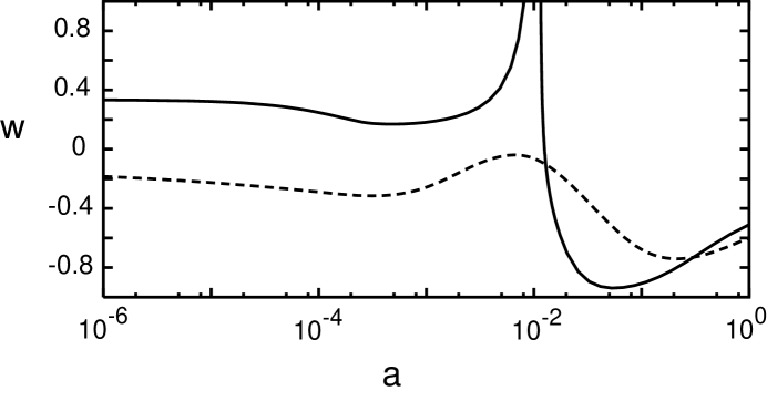
Figure 1: The equation of state for the fiducial model (solid line) and the closest spline fit (dashed line) quintessence model. The spline fit is chosen so that the CMB spectrum matches the fiducial model to within the cosmic variance limit. However, the spline itself is smoother than the actual $w(a)$. As discussed in the text, there is a large degeneracy in the spline parameters, so the spline need not mimic the fiducial equation of state very closely to obtain a good match to the CMB spectrum.

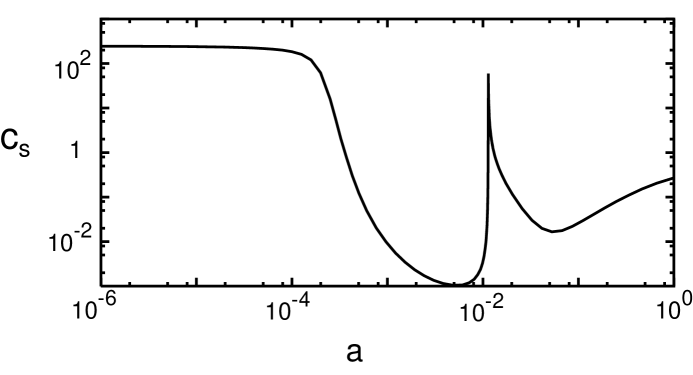
Figure 2: The speed of sound as a function of the scale factor $a$ ($a_{\text{today}}=1$). Note that at $c_{s}^{2}\ll 1$ near the last scattering surface and at the present epoch.

In the case of k-essence  the Lagrangian generally has the form $\mathcal{L}_{\phi}=\widetilde{p}(X)/\phi^{2}$, where $\widetilde{p}(X)$ is generally some function with $\widetilde{p}_{,XX}\neq 0$. We have chosen a specific form for $\widetilde{p}$ for our fiducial model. The equation of state and sound speed for this model are shown in Figs 1 and 2 respectively; they are expressed as functions of the scale factor $a$ ($a=1$ today) by integrating the equations of motion. To completely specify the model, we fix the cosmological parameters today to typical values: $\Omega_{b}=0.05$, $\Omega_{\text{CDM}}=0.3$, $\Omega_{Q}=0.65$ and $h_{0}=0.5$ (where $h_{0}$ is the Hubble parameter in units of $100\mathrm{\,km\,sec^{-1}\,Mpc^{-1}}$). The energy density as a fraction of the critical density, $\Omega_{Q}$ (k-essence), is shown in Fig. 3. While $c_{s}^{2}>1$ for large redshifts, this is not an important feature of the model: $\Omega_{Q}$ is reasonably small whenever $c_{s}^{2}>1$, so the value of $c_{s}$ at these times has negligible effect on the cmb. (We have verified this by rerunning the calculation after artificially truncating the speed of sound at $c_{s}\leq 1$ and comparing the cmb power spectra. Also, we should note that, with a slightly different parameterization, we can obtain a model in which $c_{s}<1$ which at early times and which has the same behavior at late times.) The most important feature of the fiducial model is that $c_{s}^{2}\ll 1$ whenever k-essence contributes significantly to the energy density of the universe.

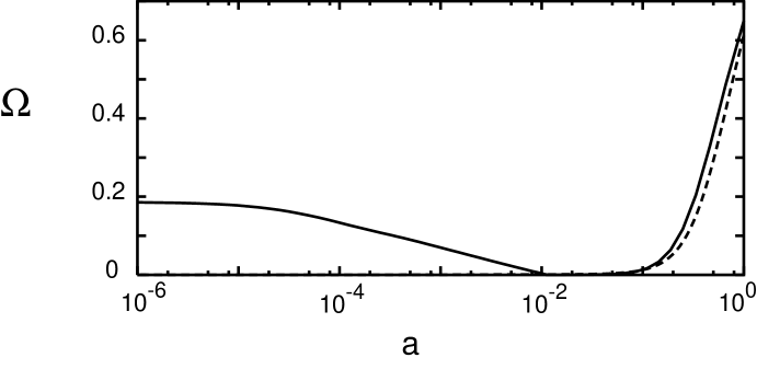
Figure 3: $\Omega_{\mathrm{\textit{k}-essence}}$ and $\Omega_{\mathrm{Q}}$ as a function of $z$ for the k-essence (solid line) and best-fit spline models (dashed line), respectively. Note that $\Omega_{Q}$ falls off to zero at large redshifts, whereas $\Omega_{\textit{k}-essence}$ approaches a finite value; $w$ approaches $1/3$ for this model at large redshifts.

The cmb power spectra for our models are computed by modifying the standard cmbfast code.Sel96 ; Cal98 Simply put, the effect of the speed of sound on the cmb perturbation equations is such that for $c_{s}^{2}\ll 1$, k-essence will collapse via gravitational instability into cold dark matter (cdm) potentials, whereas in the superluminal case, $c_{s}^{2}>1$, the growth of density perturbations is suppressed. For those familiar with the code, the modifications are straightforward. The perturbed line element is

$$ds^{2}=a^{2}(\eta)[d\eta^{2}-(\delta_{ij}+h_{ij})dx^{i}dx^{j}]$$ (4)

where $\delta_{ij}$ is the unperturbed spatial metric, and $h_{ij}$ is the metric perturbation. We shall use $h$ to represent the trace of the spatial metric perturbation. The effect we are examining is due to the perturbations to the $k$-essence stress-energy in the synchronous gauge for a mode with wavenumber $k$

$$\delta\rho = -2\rho\frac{\delta\phi}{\phi}-(\rho+p)\frac{\delta y}{y}c_{s}^{-2}$$ (5)

$$\delta p = -2p\frac{\delta\phi}{\phi}-(\rho+p)\frac{\delta y}{y}$$ (7)

$$\theta = \frac{1}{\sqrt{2}}k^{2}y\delta\phi$$ (9)

where $y\equiv 1/\sqrt{X}$ and $\theta$ is the divergence of the fluid velocity. The density contrast, $\delta\equiv\delta\rho/\rho$, obeys the equation

$$\dot{\delta}=-(1+w)\left(\theta+\frac{1}{2}\dot{h}\right)-3{\cal H}\left(\frac{\delta p}{\delta\rho}-w\right)\delta,$$ (10)

where the derivative is with respect to conformal time and ${\cal H}\equiv\dot{a}/{a}$. Notice that the quantity $\delta p/\delta\rho$ appears, which is not to be confused with $c_{s}^{2}$. In fact

$$\delta p=c_{s}^{2}\delta\rho+\frac{\theta\rho}{k^{2}}\left[3{\cal H}(1+w)(c_{s}^{2}-w)+\dot{w}\right]$$ (11)

which leads to a simplified evolution equation for the velocity gradient

$$\dot{\theta}=(3c_{s}^{2}-1){\cal H}\theta+c_{s}^{2}k^{2}\delta/(1+w).$$ (12)

The kinetic quintessence is distinct from scalar field quintessence, for which $c_{s}^{2}=1$ in equations (11) and (12). Linearized perturbations in $k$-essence can propagate non-relativistically, with $c_{s}^{2}\ll 1$. We can see in equation (12) that a small sound speed will cause the velocity gradient to decay; with the conventional gauge choice that $\theta_{cdm}=0$, the inhomogeneities in the $k$-essence will describe a fluid which is comoving with the cold dark matter. From equation (11), we see that the second term on the RHS will be negligible even on scales approaching the horizon. The overall effect is that the pressure fluctuations $\delta p$ are too weak to prevent $k$-essence collapse via gravitational instability into the CDM gravitational potentials.

The cmbfast code takes $w(a)$ and $c_{s}(a)$ as inputs, so it is possible to manually adjust these functions to have any values (including, of course, $c_{s}=1$). Once we have computed the cmb anisotropy for two models, they can be compared by computing their likelihood difference, the probability that they could be confused due to the cosmic variance in local measurements of the cmb. Given models $A$ and $B$, the negative log-likelihood, $-\log L$, is derived in Hue99 :

$$-\log L=\sum_{l}(l+{\textstyle\frac{1}{2}})\Bigl{(}1-\frac{C_{lA}}{C_{lB}}+\log\frac{C_{lA}}{C_{lB}}\Bigr{)}.$$

The condition $-\log L>6$ corresponds to distinguishability at the $3\sigma$ level or greater. The relative normalization of the spectra is chosen so as to minimize the likelihood difference, including $l$ up to $1500$.

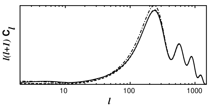
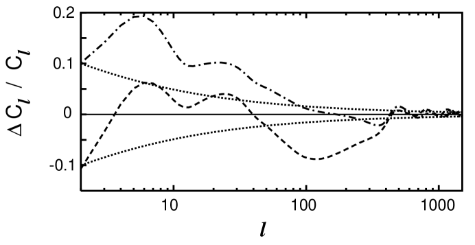
Figure 4: The CMB power spectrum for k-essence (solid line), the model with $c_{s}=1$ (dot-dashed line, $-\log L=127$) and the best-fit spline model (dashed, $-\log L=28$). Models that are distinguishable can still fit quite closely. The lower diagram shows $\Delta C_{l}/C_{l}$ (relative to the fiducial model) and the cosmic variance envelope (with no particular normalization).

The power spectrum for our fiducial model is given by the solid line in Fig. 4. We can see the effect of the unusual speed of sound on this model by computing a new spectrum, which has the same equation of state and cosmological parameters, but whose speed of sound has been set equal to $1$ for all $a$. This corresponds to a quintessence field – with canonical kinetic energy – rolling down a potential. The power spectrum for the model is shown in Fig. 4. The two models have log likelihood difference $-\log L=127$: they are easily distinguishable. The speed of sound has a significant effect on the cmb anisotropy. Figure 5 compares the dark matter and dark energy contributions for quintessence and $k$-essence models. The small sound speed results in distinctive oscillations in the case of $k$-essence.

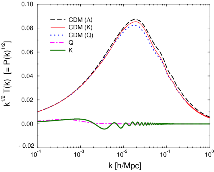
Figure 5: Comparison of the power spectra for dark matter (CDM) and dark energy ($Q$ or $K$) for models with dark energy in the form of cosmological constant ($\Lambda$), quintessence ($Q$) and $k$-essence ($K$). All models have $\Omega_{CDM}=0.3$, $\Omega_{b}h^{2}=0.02$, and $h=0.65$. For models with cosmological constant, there is no perturbed dark energy component. Note the distinctive oscillations of the $k$-essence component associated with having $c_{s}\ll 1$.

Can the effect of the sound speed be distinguished from that of other cosmological parameters? There is already a large degeneracy Hue99 in these parameters, so it would not have been too surprising if allowing a variable speed of sound merely expanded the pre-existing degeneracy. This problem is addressed by considering, as above, quintessence models which have $c_{s}^{2}=1$, but allowing the values of $\Omega_{b}$, $\Omega_{\text{CDM}}$, $\Omega_{Q}$ (quintessence) and $h_{0}$ to vary (subject to the flatness condition $\Omega_{b}+\Omega_{\text{CDM}}+\Omega_{Q}=1$). For the comparison models, the equation of state, $w$, is taken to be constant as a function of the scale factor $a$, but is allowed to vary from model to model. Minimizing the log-likelihood over these parameters, the best fit gives $-\log L=32$, with parameters $\Omega_{b}=0.05$, $\Omega_{\text{CDM}}=0.35$, $\Omega_{Q}=0.60$, $h_{0}=0.48$ and $w=-0.78$. This fit was found using well known minimization schemes. Pre93 It seems likely that $-\log L=32$ is the best that can be done for this class of models, as the result is quite insensitive to the parameter values with which the mimization is started. Hence, the speed of sound is distinguishable.

Thus far, our fiducial model has been compared with two kinds of $c_{s}=1$ models: one with all other parameters, including $w(a)$, identical and one with constant $w$, with the parameters (including $w$) adjusted so as to minimize the likelihood difference. In both cases the fiducial model was easily distinguishable. We next test the possibility that some other form of quintessence, with general $w(a)$ and canonical kinetic energy, can reproduce the cmb anisotropy of the time-varying $c_{s}$ model. For this purpose, we consider models with an equation of state given by a cubic spline.Pre93 That is, we introduce six new parameters into our model: the values of $w$ at $a=10^{-4}$, $10^{-3}$, $10^{-2}$, $10^{-1}$ and $w$ at the two extremes of $a$, which lie at $a=10^{-14}$ and $3.8$. (Introducing more spline points has a negligible effect on our results.) The equation of state at other values of $a$ is then given by a piecewise cubic (in $\log a$) function whose coefficients are chosen so that it passes through the points selected above and has a continuous second derivative. We still allow $\Omega_{b}$, $\Omega_{\text{CDM}}$, $\Omega_{Q}$ and $h_{0}$ to vary (again enforcing flatness), and now allow, for completeness, the spectral tilt $n_{s}$ to vary as well. The model therefore has a total of ten free parameters. The minimum log-likelihood difference found was $-\log L=28$, which is not a significant improvement. This model has $\Omega_{b}=0.05$, $\Omega_{\text{CDM}}=0.34$, $\Omega_{Q}=0.61$, $h_{0}=0.47$, $n_{s}=1.02$. The equation of state is shown in Fig. 1 and the cmb power spectrum is shown in Fig. 4 (dotted line).

The spline technique always produces a very smooth looking equation of state, compared to the rapidly varying equation of state (particularly near $a=0.01$) given by the actual k-essence model. To see that this does not affect the analysis – that the spline equation of state has sufficient freedom to closely mimic that for the fiducial model – we compare two models, one with $c_{s}=1$ and one with an identical speed of sound to the k-essence model. The equations of state of these models are allowed to vary using the spline technique, but the cosmological parameters are fixed to be the same as for the fiducial model. The minimum $-\log L$ for the $c_{s}=1$ model is $70$, whereas the log-likelihood difference for the model with the fiducial sound speed is much less than one. Thus, the spline technique appears to do a very good job of modeling the relevant details of the equation of state.

In sum, we have seen from our example that it is possible to distinguish models with $c_{s}=1$ (e.g. models with canonical kinetic energy density) from models with $c_{s}^{2}\ll 1$, as occurs in models with non-canonical kinetic energy density, such as k-essence. Our studies show that distinction depends on $c_{s}\ll 1$ and $\Omega_{Q}$ being at least a few percent at the last scattering surface so that the small value of the speed of sound affects the acoustic peaks, which can be precisely measured, as well as the large-angular scale anisotropy. If $\Omega_{Q}\ll 1$ at the last scattering surface, then the speed of sound only affects the large angular scale anisotropy and is difficult to distinguish because of the large cosmic variance at those scales.

As a technical device for the study, we have introduced a cubic spline method for studying varying a general equation of state $w(a)$ with a finite number of fitting quantities. The same technique can be extended to include general time-varying $c_{s}$. In this way, near-future observations of the cmb may be used to constrain general models of quintessence without introducing strong priors into its nature.

This work was supported by NSERC of Canada (JKE), NSF grant PHY-0099543 (RRC), SFB375 der Deutschen Forschungsgemeinschaft (VM), and Department of Energy grants DE-FG02-90ER4056 (CAP) and DE-FG02-91ER40671 (PJS).

References

- (1) R.R. Caldwell, R. Dave and P.J. Steinhardt, Phys. Rev. Lett. 80, 1582 (1998).
- (2) J. Frieman, C. Hill, A. Stebbins, I. Waga, Phys. Rev. Lett. 75 2077 (1995); P.J.E. Peebles and B. Ratra, Ap. J. Lett. 325, L17 (1988); B. Ratra and P.J.E. Peebles, Phys. Rev. D 37, 3406 (1988).
- (3) C. Armendariz-Picon, V. Mukhanov, and P.J. Steinhardt, Phys. Rev. Lett. 85, 4438 (2000); Phys. Rev. D 63, 103510 (2001).
- (4) G. Huey, L. Wang, R. Dave, R.R. Caldwell and P.J. Steinhardt, Phys. Rev. D 59, 063005 (1999).
- (5) Wayne Hu, Daniel J. Eisenstein, Max Tegmark, and M. White, Phys.Rev. D59 (1999) 023512; Wayne Hu, Ap. J. 506, 485 (1998).
- (6) T. Chiba, N. Sugiyama, T. Nakamura, MNRAS 301, 72 (1998).
- (7) U. Seljak and M. Zaldarriaga, Astrophys. J. 469, 437 (1996); arcturus.mit.edu:/80/matiasz/CMBFAST/cmbfast.html.
- (8) W.H. Press, S.A. Teukolsky, W.T. Vetterling, B.P. Flannery, Numerical Recipes in C: The Art of Scientific Computing, (Cambridge Univ., Cambridge, 1993).