Radioactivities and nucleosynthesis in SN 1987A

Abstract

The nucleosynthesis and production of radioactive elements in SN 1987A are reviewed. Different methods for estimating the masses of ⁵⁶Ni, ${}^{57}\rm Ni$, and ${}^{44}\rm Ti$  are discussed, and we conclude that broad band photometry in combination with time-dependent models for the light curve gives the most reliable estimates.

1 Introduction

Two of the outstanding issues for SNe are the nucleosynthesis and the explosion mechanism. Although SNe have been known from the 1950’s to be the most important sources of heavy elements, there is little quantitative evidence for this. SN 1987A has in this respect been a unique source of information thanks to the possibility to obtain spectral information at very late epochs when the ejecta is transparent and the central regions observable. The nature of the explosion mechanism is still to a large extent unknown, and constraints from observations are badly needed. The main such constraints are provided by the hydrodynamic structure, e.g., the extent of mixing, and the masses of the iron peak elements, in particular the radioactive isotopes (e.g., Timmes, Woosley, Hartmann, & Hoffman, 1996; Kumagai et al., 1993; Kifonidis, Plewa, Janka, & Müller, 2000).

2 Abundances

To model the spectra and light curve a complicated chain of thermalization processes from the gamma-rays and positrons in the keV – MeV range, to the observed optical and IR photons has to be understood. The details of this are discussed in a series of papers, (Kozma & Fransson, 1992, 1998a, 1998b). See also Fransson (1994) and de Kool, Li, & McCray (1998). Here we only summarize the main points.

After a couple of days the main energy input to the SN ejecta comes from radioactive decay, first ${}^{56}\rm Ni$ followed by ${}^{56}\rm Co$. Later than $\sim 1100$ days ${}^{57}\rm Co$ takes over, while at very late epochs, $\raise 1.29167pt\hbox{$>$}\kern-7.5pt{\lower 2.79857pt\hbox{$\sim$}}2000$ days ${}^{44}\rm Ti$  decay becomes dominant. Table 1 summarizes the different decay routes, the emitted particle (gamma-rays or positrons), the exponential decay time scale and the approximate epoch when the various decays dominated the energy input to SN 1987A.

Table 1: Main radioactive decays in SN 1987A

Decay				Time scale	Epoch when dominating
${}^{56}\rm Ni$	$\rightarrow$	$\hbox{${}^{56}\rm Co$}+\gamma$		8.8 d	0 – 18 d
		${}^{56}\rm Co$	$\rightarrow\hbox{${}^{56}\rm Fe$}+\gamma$	111.3 d	18 – 1100 d
			$\rightarrow\hbox{${}^{56}\rm Fe$}+e^{+}$
${}^{57}\rm Ni$	$\rightarrow$	$\hbox{${}^{57}\rm Co$}+\gamma$		2.17 d
		${}^{57}\rm Co$	$\rightarrow\hbox{${}^{57}\rm Fe$}+\gamma$	390 d	1100 – 1800 d
${}^{44}\rm Ti$	$\rightarrow$	$\hbox{${}^{44}\rm Sc$}+\gamma$		87 yrs	1800 d $\rightarrow$
		${}^{44}\rm Sc$	$\rightarrow\hbox{${}^{44}\rm Ca$}+\gamma$	5.4 h
			$\rightarrow\hbox{${}^{44}\rm Ca$}+e^{+}$

The gamma-rays produced by the radioactive decay loose their energy by Compton scattering off bound electrons, producing a population of non-thermal electrons in the keV range. These, as well as the positrons, are slowed down by scattering off thermal, free electrons, ionizations and excitations. This cascade has to be calculated either by Monte Carlo or by solving the Boltzmann equation, as discussed in Kozma & Fransson (1992). Knowing the heating and ionization rates, one can then calculate the temperature and ionization state of the gas, and from this the emission from the different nuclear burning zones. Finally, by solving the radiative transfer one can calculate a spectrum, which can be compared to the observations.

In figure 1 we show as an example the light curve of the ${\rm H}\alpha$  line compared to data by Danziger et al.(1991) and the SINS/HST collaboration (Wang et al.1996; Chugai et al.1997). For the explosion models we have tested both the 11E1 and 14E1 models by Shigeyama & Nomoto(1990) and the 10H model by Woosley (1988). Thge difference between these models are, however, marginal. The agreement between the model and the observations is very good over the whole evolution, which gives confidence in the whole procedure. A problem here is that a substantial fraction of the hydrogen may be at high velocity, where it is difficult to detect in the faint extended line wings. An accurate reproduction of the line profile is therefore a must in this case. In our models we find that the total mass of hydrogen rich gas is $7.7\pm 2~{}M_{\odot}$, of which $\sim 2.2~{}M_{\odot}$ is mixed within 2000 $\rm~{}km~{}s^{-1}$. Of the hydrogen rich gas $\sim 3.9~{}M_{\odot}$ is helium, while an equal mass is hydrogen.

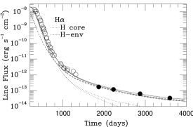
Figure 1: Left panel: Evolution of H$\alpha$ from Danziger et al.  and from SINS/HST observations together with model calculations. The flat tail is mainly a result of freeze-out rather than input from ⁴⁴Ti, as can be seen from the dominance of the low density envelope (dashed line), compared to the higher density core (dotted). Right panel: Evolution of the ’6300 Å’ line. At early epochs the [O I] $\lambda\lambda 6300,6364$ lines dominate (dotted line), while most of the flux at epochs $\raise 1.29167pt\hbox{$>$}\kern-7.5pt{\lower 2.79857pt\hbox{$\sim$}}1400$ days originates from an Fe I line at 6300 Å. The oxygen mass was in this model $1.9~{}M_{\odot}$.

The mass of the helium dominated zone is consistent with $\sim 1.9~{}M_{\odot}$, of which $\sim 1.8~{}M_{\odot}$ is pure helium, with a further $\sim 3.9~{}M_{\odot}$ of helium residing in the hydrogen component. A possible caveat is again that a substantial mass could be hidden at velocities $\raise 1.29167pt\hbox{$>$}\kern-7.5pt{\lower 2.79857pt\hbox{$\sim$}}~{}3000\rm~{}km~{}s^{-1}$.

Oxygen is important both as a diagnostic of the evolutionary calculations, the progenitor mass, and because of its large abundance. In figure 1, right panel, we show the corresponding light curve for this line. A technical point is here that while the feature at $\sim 6300$ Åis dominated by the [O I] $\lambda\lambda 6300,6364$ doublet at epochs $\raise 1.29167pt\hbox{$<$}\kern-7.5pt{\lower 2.79857pt\hbox{$\sim$}}1000$ days, it is at late time instead dominated by an Fe I line at $6300$ Å. This illustrates the importance of a self-consistent calculation of the spectrum, taking all important ions and transitions into account. The total oxygen mass we find is $\sim 1.4~{}M_{\odot}$, but the permissible range is probably as large as $0.7-3.0~{}M_{\odot}$. One can from this with good confidence rule out progenitor models with ZAMS mass less than $15~{}M_{\odot}$, because of the low oxygen mass ($\raise 1.29167pt\hbox{$<$}\kern-7.5pt{\lower 2.79857pt\hbox{$\sim$}}~{}0.5~{}M_{\odot}$).

In table 2 we summarize the most important masses derived from the spectra and light curves (bolometric and broad band UBVRI). The latter are discussed in section 3. Other elements are discussed in Kozma & Fransson (1998b).

Table 2: Masses of some important elements and isotopes in SN 1987A.

Isotope	Mass ($~{}M_{\odot}$)		Method	Note
${}^{1}\rm H$	3.	9	Spectrum
${}^{4}\rm He$	5.	8	Spectrum
${}^{16}\rm O$	1.	9	Spectrum
$\hbox{${}^{56}\rm Ni$}~{}~{}(\hbox{${}^{56}\rm Fe$})$	0.	069	Bol. l.c.	$\pm 0.003~{}M_{\odot}$
$\hbox{${}^{57}\rm Ni$}~{}~{}(\hbox{${}^{57}\rm Fe$})$	0.	003	UBVRI l.c.
${}^{58}\rm Ni$	0.	006	Spectrum
$\hbox{${}^{44}\rm Ti$}~{}~{}(\hbox{${}^{44}\rm Ca$})$	0.	0001	UBVRI l.c.	$(0.5-2)\times 10^{-4}~{}M_{\odot}$

3 The radioactive isotopes and the light curve.

To estimate the masses of the three most abundant radioactive isotopes formed in the explosion, ⁵⁶Ni, ${}^{57}\rm Ni$  and ${}^{44}\rm Ti$ , one can use several approaches, each with its special advantages and disadvantages (Fransson & Kozma, in preparation). The best known, and for the ⁵⁶Ni mass most reliable, is the bolometric light curve. As shown by e.g., Bouchet et al. (1991), this yields a ⁵⁶Ni  mass of $0.069~{}M_{\odot}$.

For ${}^{57}\rm Ni$, or rather, ${}^{57}\rm Co$, which dominates the light curve between 1100 – 1800 days, this is not so straightforward, and a simple approach similar to that of ${}^{56}\rm Co$, yielded a ${}^{57}\rm Ni$  mass at least twice as large as other methods, and much higher than could be produced by the nucleosynthesis models (Suntzeff et al., 1992; Bouchet, Danziger, & Lucy, 1991). This was shown by Fransson & Kozma (1993) to be a result of time dependent effects in the light curve. Because of the decreasing density and ionization, the recombination time scale ($\propto 1/(\alpha_{rec}n_{e})$) as well as the cooling time scale, become longer than the expansion time scale, $t$. The gas is therefore not able to recombine and cool at the same rate as the radioactive input takes place, and only a fraction of the radioactive input is released as radiation. The difference is released later as recombination radiation, giving a higher luminosity than the instantaneous input. The bolometric light curve therefore gives an overestimate of the radioactive mass if a simple steady state calculation is employed.

In figure 2 we show a time dependent calculation of the bolometric light curve, and also showing the various individual radioactivity contributions. When we compare the bolometric luminosity with the total energy input one sees that between $\sim 1200$ days and $\sim 2500$ days the bolometric luminosity is up to a factor three higher than the input. At very late time most of the energy input is in the iron rich zones by positrons from ${}^{44}\rm Ti$, making time dependent effects less important.

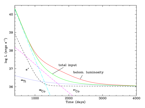
Figure 2: Bolometric light curve of SN 1987A with M$({}^{56}$Co$)=0.07~{}M_{\odot}$, M$({}^{57}$Co$)=3.3\times 10^{-3}~{}M_{\odot}$, and M$({}^{44}$Ti$)=1\times 10^{-4}~{}M_{\odot}$. The separate contributions from the different isotopes as well as the positron input are shown as dashed and dotted lines. Note the dominant positron input from ${}^{44}\rm Ti$  at late epochs.

The most serious problem of using the bolometric light curve at late times is the large bolometric correction necessary because nearly all of the emission emerges in the unobserved far-IR. In figure 3 we nevertheless show the time-dependent bolometric light curve. This represents an extension of the modeling in Fransson & Kozma (1993) to later epochs, and with updated physics. The freeze-out increases in this case the luminosity by a factor 2 – 3 at epochs later than 1200 days. The observations come from CTIO data by Suntzeff et al. (1992), and ESO data by Danziger & Bouchet (1993). While the agreement with the CTIO data is good, the agreement is considerably worse with the ESO data during the late epochs. The discrepancy between the ESO and CTIO data probably gives a good estimate of the systematic errors in the observations, and it is clear that a different approach has to be taken for estimating the mass of ${}^{44}\rm Ti$, and also to get a more accurate estimate of the ${}^{57}\rm Ni$  mass.

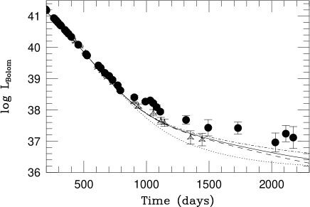
Figure 3: Bolometric light curve with M$({}^{56}$Co$)=0.07~{}M_{\odot}$, M$({}^{57}$Co$)=3.3\times 10^{-3}~{}M_{\odot}$, and M$({}^{44}$Ti$)=1\times 10^{-4}~{}M_{\odot}$. Data are from Danziger & Bouchet (1993) (dots) and from Suntzeff et al.(1992) (triangles). The dotted line gives the steady state light curve, while the solid shows the same with time dependent effects included.

The second approach involves modeling of the line emission from the ejecta. An example of this was shown in figure 1, where we show ${\rm H}\alpha$  light curves for three different values of the ${}^{44}\rm Ti$  mass. . Although the model reproduces the observations very well during the whole evolution, as a measure of the ⁴⁴Ti mass the light curve is clearly not very sensitive. Nearly all of the excitation is due to gamma-rays absorbed by the envelope, and the line is therefore strongly affected by the freeze-out. Most of the emission at $\raise 1.29167pt\hbox{$<$}\kern-7.5pt{\lower 2.79857pt\hbox{$\sim$}}~{}3000$ days is in fact due to the delayed recombination from the epoch at $\raise 1.29167pt\hbox{$<$}\kern-7.5pt{\lower 2.79857pt\hbox{$\sim$}}~{}2000$ days when ⁵⁷Co dominated the energy input. A better alternative is to use lines from the metal rich core, in particular the Fe I and Fe II lines. An important result found by Chugai et al.(1997) is that in order to reproduce the Fe II flux, positrons have to be trapped efficiently in the iron rich gas. Pure Coulomb collisions are not sufficient for this, but a weak magnetic field is enough to make the gyro radius of the positrons small enough. A severe problem is, however, that modeling of individual lines is very sensitive to atomic data, which in spite of dramatic improvements from the IRON-project, is still a problem. In a similar attempt Lundqvist et al. (2001) have tried to use the FIR [Fe II] $26.0\mu$ fine structure line in connection with observations by ISO. Unfortunately, only an upper limit to the flux was obtained, yielding an upper limit to the ${}^{44}\rm Ti$  mass of $1.1\times 10^{-4}~{}M_{\odot}$. There is, however, a number of loop holes in this result, such as extra dust cooling, mixing with other heavy elements contributing to the cooling like silicon and sulphur, as well as uncertainties in the atomic data.

A compromise between these two approaches is offered by broad band photometry, where photometry in the optical and near-IR is compared to synthetic photometry from spectral calculations. This method avoids the need to extrapolate into the far-IR for the bolometric light curve, as well as many of the uncertainties involved in the calculation of individual lines. Rather than modeling individual lines, the broad band fluxes are mainly sensitive to the division between UV, optical and IR in the spectral distributions of the elements. This is determined by the atomic configuration, i.e. the term diagram, and less by the exact path a recombining photon takes when cascading to the ground state. Except for the fraction of the emission in the optical and IR which is absorbed by the dust, the photometry is insensitive to this component. The fraction absorbed by dust can be estimated from mid-IR observations, as well as from line profile shifts (Lucy et al.1991).

In figure 4 we show the B and V band light curves together with observations. The reason for concentrating on these bands is that they are strongly dominated by lines from Fe I and Fe II, and therefore most sensitive to the ${}^{44}\rm Ti$  mass, in contrast to the R band which is dominated by ${\rm H}\alpha$, and therefore sensitive to the freeze out. Observations are taken from Suntzeff et al.(1991) and HST observations from Suntzeff et al.(2001). The models have $6.9\times 10^{-2}~{}M_{\odot}$ of ⁵⁶Co, $3.3\times 10^{-3}~{}M_{\odot}$ of ⁵⁷Co and three different values of the ${}^{44}\rm Ti$  mass, $(0.5,1.0,2.0)\times 10^{-4}~{}M_{\odot}$. As can be seen, both the B and V bands are well reproduced by the observations throughout the whole evolution, and the currently best estimate of the ${}^{44}\rm Ti$ mass is in the range $(0.5-2.0)\times 10^{-4}~{}M_{\odot}$. This method also yields the best estimate of the ${}^{57}\rm Ni$  mass, $\sim 3.3\times 10^{-3}~{}M_{\odot}$. A more complete discussion of these results will be given in Fransson & Kozma (2001).

Figure 4: B and V light curves from Suntzeff et al.(1991, 2001), together with models with $(0.5,1.0,2.0)\times 10^{-4}~{}M_{\odot}$ of ⁴⁴Ti. All models have $3.3\times 10^{-3}~{}M_{\odot}$ of ⁵⁷Ni

4 Conclusions

SN 1987A is by far the best source of nucleosynthesis of any SN. Reliable masses for both the most abundant elements, H, He, and O, as well as the the most abundant radioactive isotopes, ⁵⁶Ni, ${}^{57}\rm Ni$, and ${}^{44}\rm Ti$  have been obtained. These provide some of the most important constraints on the progenitor and on the explosion itself.

CF is grateful to Roland Diehl for organizing a very successful workshop, and to Don Clayton and Nikos Prantzos for useful discussions and comments.

References

- Bouchet & Danziger (1993) Bouchet, P. & Danziger, I. J. 1993, A&A, 273, 451
- Bouchet, Danziger, & Lucy (1991) Bouchet, P., Danziger, I. J., & Lucy, L. B. 1991, AJ, 102, 1135
- Bouchet et al. (1991) Bouchet, P., Phillips, M. M., Suntzeff, N. B., Gouiffes, C., Hanuschik, R. W., & Wooden, D. H. 1991, A&A, 245, 490
- Chugai, Chevalier, Kirshner, & Challis (1997) Chugai, N. N., Chevalier, R. A., Kirshner, R. P., & Challis, P. M. 1997, ApJ, 483, 925
- Danziger & Bouchet (1993) Danziger, I. J. & Bouchet, P. 1993, New Aspects of Magellanic Cloud Research, 208
- Danziger et al. (1991) Danziger, I. J., Bouchet, P., Gouiffes, C., Lucy, L. B. 1991, in Proc. ESO/EIPC Supernova Workshop, SN 1987A and other Supernovae, eds. I.J. Danziger & K. Kjär, (Garching: ESO), 217
- de Kool, Li, & McCray (1998) de Kool, M., Li, H., & McCray, R. 1998, ApJ, 503, 857
- Fransson (1994) Fransson, C., 1994, in Supernovae (Les Houches, Session LIV 1990), eds. J. Audouze, S. Bludman, R. Mochkovitch, & J. Zinn-Justin (New York: Elsevier), 677
- Fransson & Kozma (1993) Fransson, C. & Kozma, C. 1993, ApJ Lett, 408, L25
- Kifonidis, Plewa, Janka, & Müller (2000) Kifonidis, K., Plewa, T., Janka, H.-T., & Müller, E. 2000, ApJ Lett, 531, L123
- Kozma & Fransson (1992) Kozma, C. & Fransson, C. 1992, ApJ, 390, 602
- Kozma & Fransson (1998a) Kozma, C. & Fransson, C. 1998, ApJ, 496, 946
- Kozma & Fransson (1998b) Kozma, C. & Fransson, C. 1998, ApJ, 497, 431
- Kumagai et al. (1993) Kumagai, S., Nomoto, K., Shigeyama, T., Hashimoto, M., & Itoh, M. 1993, A&A, 273, 153
- Lucy, Danziger, Gouiffes, and Bouchet (1991) Lucy, L.B., Danziger, I.J., Gouiffes, C., and Bouchet, P. 1991, in Supernovae, Proc. of the Tenth Santa Cruz Summer Workshop in Astronomy and Astrophysics, ed. S.E. Woosley (Springer Verlag), 82.
- Lundqvist et al. (2001) Lundqvist, P., Kozma, C., Sollerman, J. & Fransson, C. 2001, A&A, 374, 629
- Phillips et al. (1990) Phillips, M. M., Hamuy, M., Heathcote, S. R., Suntzeff, N. B., & Kirhakos, S. 1990, AJ, 99, 1133
- Shigeyama & Nomoto (1990) Shigeyama, T. & Nomoto, K. 1990, ApJ, 360, 242
- Suntzeff et al. (1991) Suntzeff, N. B., Phillips, M. M., Depoy, D. L., Elias, J. H., & Walker, A. R. 1991, AJ, 102, 1118
- Suntzeff et al. (1992) Suntzeff, N. B., Phillips, M. M., Elias, J. H., Walker, A. R., & Depoy, D. L. 1992, ApJ Lett, 384, L33
- Suntzeff et al. (2001) Suntzeff, N. B. et. al. 2001, in preparation
- Timmes, Woosley, Hartmann, & Hoffman (1996) Timmes, F. X., Woosley, S. E., Hartmann, D. H., & Hoffman, R. D. 1996, ApJ, 464, 332
- Wang et al. (1996) Wang, L. et al. 1996, ApJ, 466, 998
- Woosley (1988) Woosley, S. E. 1988, ApJ, 330, 218