Quest for HI Turbulence Statistics: New Techniques
Abstract
HI data cubes are sources of unique information on interstellar turbulence. Doppler shifts due to supersonic motions contain information on turbulent velocity field which is otherwise difficult to obtain. However, the problem of separation of velocity and density fluctuations within HI data cubes is far from being trivial. Analytical description of the emissivity statistics of channel maps (velocity slices) in Lazarian & Pogosyan (2000) showed that the relative contribution of the density and velocity fluctuations depends on the thickness of the velocity slice. In particular, power-law assymptotics of the emissivity fluctuations change when the dispersion of the velocity at the scale under study becomes of the order of the velocity slice thickness (integrated width of the channel map). These results are the foundations of the Velocity-Channel Analysis (VCA) technique which allows to determine velocity and density statistics using 21-cm data cubes. The VCA has been successfully tested using data cubes obtained via compressible magnetohydrodynamic simulations and applied to Galactic and Magellanic Clouds data. As a tool it has become much more sophisticated recently when effects of absorption were accounted for. The systematic studies of vast 21-cm data sets to correlate the variations in the turbulence statistics with the astrophysical activity is on the agenda. This should allow to determine the interstellar energy injection mechanisms. Going beyond the VCA, we discuss other tools, namely, genus and anisotropy analysis. The first characterises the topology of HI, while the second provides magnetic field directions. We show a few applications of these new tools to HI data and MHD simulations.
University of Wisconsin-Madison, USA; lazarian@astro.wisc.edu
University of Alberta, Canada; pogosyan@Phys.UAlberta.CA
University of Wisconsin-Madison, USA; esquivel@astro.wisc.edu
1. Introduction
Atomic hydrogen is an important component of the interstellar media of spiral galaxies (McKee & Ostriker 1977) and much efforts have been devoted to its studies (see this volume). From the point of view of fluid mechanics, HI, as well as other components of interstellar medium, is characterised by huge Reynolds numbers, , which is the ratio of the eddy turnover time of a parcel of gas to the time required for viscous forces to slow it appreciably. For we expect gas to be turbulent and this is exactly what we observe in HI (for HI ).
Statistical description is a nearly indispensable strategy when dealing with turbulence. The big advantage of statistical techniques is that they extract underlying regularities of the flow and reject incidental details. Attempts to study interstellar turbulence with statistical tools date as far back as the 1950s (see Horner 1951, Kampe de Feriet 1955, Munch 1958, Wilson et al. 1959) and various directions of research achieved various degree of success (see reviews by Kaplan & Pickelner 1970, Dickman 1985, Lazarian 1992, Armstrong, Rickett & Spangler 1995). Studies of turbulence statistics of ionized media were successful (see Spangler & Gwinn 1990) and provided the information of the statistics of plasma density at scales - cm. This research profited a lot from clear understanding of processes of scintillations and scattering achieved by theorists (see Narayan & Goodman 1989). At the same time the intrinsic limitations of the scincillations technique are due to the limited number of sampling directions, relevance only to ionized gas at extremely small scales, and impossibility of getting velocity (the most important!) statistics directly.
“Seeing through dust” at 21 cm potentially provides an enormous leap for turbulence studies. First of all, statistics of HI line carries the velocity information. Secondly, the statistical samples are extremely rich and not limited to discrete directions. Thirdly, HI emission allows to study turbulence at large scales which have direct relation to the scales of star formation and energy injection.
Deficiencies in the theoretical description has been, to our mind, the major impediment to studies of turbulence using 21-cm data cubes. In particular, Crovisier & Dickey (1983) Green (1993) measured the spectrum of 21-cm intensity fluctuations, but it was unclear what those spectra mean.
Sally Oey (this volume) identifies several known problems of studying HI turbulence. They are (a) integration of fluctuations along lines of sight, (b) contribution of velocity and density to the emissivity statistics and (c) effects of absorption. The problems related to (a) were dealt in Lazarian (1995), while the issues (b) and (c) happen to be more formidable and have been dealt with only recently (Lazarian & Pogosyan 2000, 2002). Earlier reviews dealing with HI studies include Lazarian (1999a,b). In this volume one can read more about turbulence in Cho, Lazarian & Yan and Vazquez-Semadeni papers.
2. Statistics of HI Data Cubes and Velocity Channel Analysis
Doppler shifted spectral lines carry information about turbulent velocity, but until very recently there was no way of extracting this information. The problem is that both velocity and density fluctuations contribute to the fluctuations of the intensity at a given velocity. In other words: We know the statistics of spectral lines, i.e. the statistics in velocity space, while we want to determine the actual 3D statistics.
Statistics in 3D
Turbulence theory deals with the statistics of turbulence in real space that
can be described by 3D correlation and structure functions (see
Monin & Yaglom 1975). For instance,
if density correlation function (CF) is isotropic in -space then
| (1) |
The power spectrum provides an alternative description and is related to the correlation function as
| (2) |
where integration is performed over the 3D space. For power-law statistics, the dimensional power spectrum and correlation function have indexes related as . In other words,
| (3) |
Statistics in Position Position Velocity (PPV) Space
One does not observe the gas distribution in the real space galactic
coordinates . Rather, intensity of the emission in a given spectral
line is measured towards some direction on the sky and at a
given line-of-sight velocity .
In the plane parallel approximation the direction on the sky can be identified
with the 2D spatial vector perpendicular to the line of sight,
so that the coordinates of experimental PPV cubes are .
If we chose galactic coordinates so that specify the direction of
observation and is the coordinate along the line of sight
, then the relation between the
real space and the PPV descriptions
is that of a map .
The line-of-sight component of velocity at the position is a sum of the regular gas flow (e.g., due to galactic rotation) , the turbulent velocity and the residual component due to thermal motions. The thermal velocity has Maxwellian distribution
| (4) |
where , is the atomic mass and is the gas temperature.
The density of emitters in the PPV space can then be written as
| (5) |
where is the density of gas in the galactic coordinates. This expression just counts the number of atoms along the line-of-sight X which have z-component of velocity in the interval The limits of integration are defined by the extend of spatial distribution of emitting gas.
The statistics available in PPV are the correlation functions
and the power spectra of the emissivity fluctuations.
The latter may be 3D, 2D and 1D. The relation between those spectra and the
underlying velocity and density spectra were established in Lazarian & Pogosyan (2000). In practical
terms, the most frequently used is the 2D spectrum of velocity slices. This
spectrum can be directly obtained with radiointerferometric observations (see
Lazarian 1995).
Velocity-Channel Analysis (VCA)
The VCA technique has been developed
in Lazarian & Pogosyan (2000, henceforth LP00)
for analyzing line
profile formation in the presence of turbulence. We have predicted
analytically that the relative contribution of the velocity and density
fluctuations to the total fluctuations of intensity changes
in a regular fashion with the width of the velocity slice.
This is easy to understand
qualitatively, as it is clear that the line integration should decrease
the influence of velocity fluctuations. We have shown
that if the 3-D density spectrum
is (where is the wavenumber),
two distinct regimes are present when: (a) , and (b) .
Our results are summarized in Table 1.
| Slice | Shallow 3-D density | Steep 3-D density |
|---|---|---|
| thickness | , | , |
| 2-D intensity spectrum for thina slice | ||
| 2-D intensity spectrum for thickb slice | ||
| 2-D intensity spectrum for very thickc slice |
It is easy to see that both in cases (a) and (b) the power law index gradually steepens with the increase of velocity slice thickness. In the thickest velocity slices the velocity information is averaged out and it is natural that we get the density spectral index . The velocity fluctuations dominate in thin slices, and if the 3-D velocity power spectrum is , then the index can be found from thin slices (see Table 1). Note, that the notion of thin and thick slices depends on a turbulence scale under study and the same slice can be thick for small scale turbulent fluctuations and thin for large scale ones. The formal criterion for the slice to be thick is that the dispertion of turbulent velocities on the scale studied should be less than the velocity slice thickness. Otherwise the slice is thin.
Predictions of LP00 were tested in Lazarian et al. (2001) using numerical MHD simulations of compressible intersterllar gas. Simulated data cubes allowed both density and velocity statistics to be measured directly. Then these data cubes were used to produce synthetic spectra which were analysed using the VCA. As the result, the velocity and density statistics were successfully recovered. Thus one can confidently apply the technique to HI observations. Note, that the VCA is only sensitive to velocity111For Kolmogorov turbulence the velocity gradient scales as . and density gradients on the scale under study, so the regular Galactic rotation curve or large scale distribution of emitting gas does not interfere with the analysis.
Further research in Lazarian & Pogosyan (2002) incorporated the effects of absorption into the VCA. Namely, we have shown that in the presence of strong absorption a universal spectrum with index is being produced in very thick slices, provided that the density is steep. The universality means that the emissivity spectral index does not depend on the underlying statistics of velocity and density. For shallow density, its spectral index determines the emissivity statistics. To get velocity information thin slices must be used.
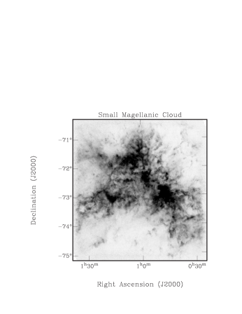
3. Applications of the VCA: SMC and Galactic HI
In the case of SMC the VCA reveals the Kolmogorov-type spectrum, (where is the energy contained in eddies with (eddy size)-1) for velocity fluctuations and a slightly more shallow spectrum of density fluctuations over the range of scales from 4 kpc to 40 pc.

A spectral index similar to the one for SMC has been inferred from the 21 cm Galactic data in Green (1993). However, that index shows more variability, which can stem from a number of causes. First of all, LP00 predicts, and the analysis of Fig. 1 confirms, that the emissivity index depends on whether or not the velocity dispersion on the scale under study is larger or smaller than the thickness of the channel map. In Green (1993) the physical scales and therefore the associated velocity dispersion vary considerably for close and distant slices of HI. Moreover, for the close slices the geometry of parallel lines of sight adopted in LP00 does not provide a good approximation and the convergence of the lines of sight must be accounted for.
The situation is even more complicated for the inner parts of the Galaxy, where (a) two distinct regions at different distances from the observer contribute to the emissivity for a given velocity and (b) effects of the absorption are important. However, the analysis in Dickey et al. (2001) showed that some progress may be made even in those unfavorable circumstances. Dickey et al. (2001) found the steepening of the spectral index with the increase of the velocity slice thickness. They also observed the spectral index for strongly absorbing direction approached in accordance with the conclusions in Lazarian & Pogosyan (2002).
21-cm absorption provides another way of probing turbulence on small scales. The absorption depends on the density to temperature ratio , rather than to as in the case of emission. However, in terms of the VCA this change is not important and we still expect to see emissivity index steepening as velocity slice thickness increases, provided that velocity effects are present. In view of this, results of Deshpande et al. (2001), who did not see such steepening, can be interpreted as the evidence of the viscous suppression of turbulence on the scales less than 1 pc. The fluctuations in this case should be due to density and their shallow spectrum may be related to the damped magnetic structures below the viscous cutoff (see Cho, Lazarian, Yan, this volume).
Clearly, more VCA studies of Galactic HI are required. As the VCA can be used for other emission lines (e.g. CO, Hα), cross-correlation of turbulence properties in HI, molecular and ionized gas is necessary to obtain an insight into the dynamic coupling of different interstellar phases.
4. Complementary Statistical Tools
Genus Analysis
Velocity and density power spectra do not provide the complete description
of turbulence. Intermittency of turbulence (its variations in time and space)
and its topology in the presence of different phases are
not described by the power spectrum.
“Genus analysis” is a good tool for studying the topology of turbulence (see review by Lazarian 1999), receiving well-deserved recognition for cosmological studies (Gott et al. 1989). Consider an area on the sky with contours of projected density. The 2D genus, , is the difference between the number of regions with a projected density higher than and those with densities lower than . Fig. 4 shows the 2D genus as the function of for a Gaussian distribution of densities (completely symmetric curve), for MHD isothermal simulations with Mach number 2.5, and for HI in SMC (Fig. 4b).


Isothermal MHD simulations exhibit more or less symmetric density distributions, but the SMC data reflect a prominent Swiss cheese topology, which also can be suggested from the visual inspection of the image (see Fig. 3). However, unlike visual inspection, the genus quantifies the topology and allows us to compare numerical results with observations. Note, that the MHD simulations in Fig 4a are not so different from the SMC in terms of the power spectrum.
Anisotropy Analysis
In isotropic turbulence, correlations depend only on the distance
between the points. Contours of equal correlation are
circular in this case. Presence of magnetic field introduces anisotropy
and these contours become elongated with a symmetry axis given by
the magnetic field. To study turbulence
anisotropy, we can measure contours of equal correlation corresponding
to the data within various
velocity bins. The results obtained with simulated data are shown in Fig. 3.


Since the anisotropy is related to the magnetic field, the studies of anisotropy can provide means to analyze magnetic fields. It is important to study different data sets and channel maps for the anisotropy. Optical and infrared polarimetry can benchmark the anisotropies in correlation functions. We hope that the anisotropies will reveal magnetic field within dark clouds where grain alignment and therefore polarimetry fails (see Lazarian 2000, astro-ph/0003314 for a review of grain alignment).
5. Summary
For the first time ever we have an adequate theoretical description of spectral line statistics in the presence of both velocity and density fluctuations. This must be exploited to get adequate description of interstellar turbulence. HI data cubes present a great opportunity for such a study. To get a better understading of interstellar dynamics we propose using complementary tools like genus and anisotropy analysis and correlating the statistics of HI with that of molecular species and ions.
Acknowledgement. AL acknowledges the support by the grant NSF AST-0125544.
References
Armstrong, J.M., Rickett, B.J., & Spangler, S.R. 1995, ApJ, 443, 209
Cho, J., Lazarian, A., & Vishniac, E. 2002, ApJ, 564, 000
Crovisier, J. & Dickey, J. M. 1983, A&A, 122, 282
Deshpande, A.A., Dwarakanath, K.S., Goss, W.M., 2000, ApJ, 543, 227
Green, D.A. 1993 MNRAS, 262, 328
von Horner, S. 1951, Zs.F. Ap., 30, 17
Kaplan, S.A. & Pickelner, S.B. 1970, The Interstellar Medium, Harvard Univ. Press
Lazarian, A. 1992, Astron. and Astrophys. Transactions, 3, 33
Lazarian, A. 1995, A&A, 293, 507
Lazarian, A. 1999a, Turbulence in Atomic Hydrogen, in Interstellar Turbulence, eds. Jose Franco & Alberto Carraminana, CUP, p.95
Lazarian, A. 1999b, Statistics of Turbulence from Spectral-Line Data Cubes, in Plasma Turbulence and Energetic Particles, ed. M. Ostrowski and R. Schlickeiser, Cracow, 28, astro-ph/0001001
Lazarian, A. & Pogosyan, D. 2000, ApJ, 537, 720
Lazarian, A., Pogosyan, D., Vazquez-Semadeni,E., & Pichardo, B. 2001, ApJ, 555, 130
Monin, A.S., & Yaglom, A.M. 1975, Statistical Fluid Mechanics: Mechanics of Turbulence, vol. 2, The MIT Press
Munch, G. 1958, Rev. Mod. Phys., 30, 1035
Narayan, R., & Goodman, J. 1989, MNRAS, 238, 963
Stanimirovic, S., & Lazarian, A. 2001, ApJ, 551, L53
Spangler, S.R., & Gwinn, C.R. 1990, ApJ, 353, L29
Wilson, O.C., Munch, G., Flather, E.M., & Coffeen, M.F. 1959, ApJS, 4, 199