Deep HST-WFPC2 photometry of NGC 288. I.
Binary Systems and Blue Stragglers

Abstract

We present the first results of a deep WFPC2 photometric survey of the loose galactic globular cluster NGC 288. The fraction of binary systems is estimated from the color distribution of objects near the Main Sequence (MS) with a method analogous to that introduced by Rubenstein & Bailyn (1997). We have unequivocally detected a significant population of binary systems which has a radial distribution that has been significantly influenced by mass segregation. In the inner region of the cluster ($r<1r_{h}\simeq 1.6r_{c}$) the binary fraction ($f_{b}$) lies in the range 0.08–0.38 regardless of the assumed distribution of mass ratios, $F(q)$. The most probable $f_{b}$ lies between 0.10 and 0.20 depending on the adopted $F(q)$. On the other hand, in the outer region ($r\geq 1r_{h}$), $f_{b}$ must be less than 0.10, and the most likely value is 0.0, independently of the adopted $F(q)$. The detected population of binaries is dominated by primordial systems.

The specific frequency of Blue Straggler Stars (BSS) is exceptionally high, suggesting that the BSS production mechanism via binary evolution can be very efficient. A large population of BSS is possible even in low density environments if a sufficient reservoir of primordial binaries is available. The observed distribution of BSS in the Color Magnitude Diagram is not compatible with a rate of BSS production which has been constant in time, if it is assumed that all the BSS are formed by the merging of two stars.

1 Introduction

Binary systems are the most frequent form in which stars present themselves, at least in our local neighborhood (Duquennoy & Mayor, 1991), and it is generally believed that the same process of stellar birth commonly takes place in clusters (e.g., Mathieu, 1996, and references therein). Furthermore, binaries have a significant impact on the chemical evolution of galaxies and even toy chemical evolution models can easily show that our Universe would not have been as it is without them (Portegies Zwart, Yungelson & Nelemans, 2000).

In collisional stellar systems, binaries can play a key role also in the dynamical evolution. In particular, binaries provide the gravitational fuel that stops and eventually reverses the process of core collapse in globular clusters (Hut et al., 1992; Meylan & Heggie, 1997, and references therein). Moreover, the evolution of binaries in clusters can produce peculiar stellar species such as Blue Stragglers (BSS), Cataclysmic Variables (CV), Low Mass X ray sources (LMXB), millisecond pulsars (MSP) and possibly sdB (Bailyn, 1995; Portegies Zwart, Hut & Verbunt, 1997a; Portegies Zwart et al., 1997b; Saffer, Green & Bowers, 2001; Maxted et al., 2001; Green, 2001; Green, Liebert, & Saffer, 2001). Thus, the study of binary populations in globular clusters can provide powerful constraints both on dynamical models or on models of formation of exotic objects.

Despite their potential interest, the actual detection of binaries and estimate of the binary fraction ($f_{B}$) in globular clusters has eluded the effort of researchers until very recent times (see Hut et al., 1992; Gunn & Griffin, 1979; Irwin & Trimble, 1984), because of the challenging observational requirements.

There are three main techniques which have been used to detect binary populations in globular clusters (reviewed by (Hut et al., 1992)): (i) radial velocity variability surveys (Latham, 1996), (ii) searchs for eclipsing variables (Mateo, 1996a), and (iii) searches for a Secondary Main Sequence (SMS, see Romani & Weinberg, 1991; Hurley & Tout, 1998) parallel to the normal Main Sequence (MS) in the Color Magnitude Diagram (CMD).

Methods (i) and (ii) are based on the actual detection of individual binary systems. They require large amounts of observing time, since time series are necessary. Method (i) also requires very high precision radial velocity measures that limit the luminosity range of the targets and place great demands on the quality and stability of the instrumental setup. These lead to observational biases and intrinsic limitations (see §2.1 and §2.2 in Hut et al., 1992) and ultimately to a low discovery efficiency. Thus, while these methods provide the only route to the physical characterization of individual systems (masses, orbits etc.), they are maladapted to determining population properties, such as the binary fraction.

In contrast, method (iii) is statistical in nature and does not need repeated observations. It is based on the simple fact that any binary system at the distance of globular clusters is seen as a single star with a flux equal to the sum of the fluxes of the two components. In the CMD, systems composed of two equal mass MS stars lie on a sequence $0.752$ mag brighter than the single stars sequence. If the masses are not equal the shift away from the MS is smaller and depends non-linearly on the mass ratio of the two components, $q={M_{2}\over{M_{1}}}\leq 1.0$ (see Hurley & Tout, 1998), where $M_{1}$ and $M_{2}$ are the mass of the primary and secondary stars, respectively.

While the SMS can detect binaries of any orbital period and any orientation of the orbital plane, it suffers from three problems:

• The observational signatures of a genuine binary system and two blended, but unrelated, single stars are indistinguishable. Thus, any SMS in a globular cluster is contaminated to some degree by blended objects.

• Exceptionally accurate photometry extending to at least a couple of magnitudes below the Turn Off point (TO) is required. Any secondary sequence can be easily obscured by the observational scatter in the single star sequence. Thus, while hints of a SMS have been found in many cases (see Tab. 3 in Hut et al., 1992), the only definitive detections from ground based photometry have been in two very loose and relatively nearby clusters, E3 (Veronesi et al., 1996; McClure et al., 1985) and NGC 288 (Bolte, 1992).

• The distribution of mass ratios must be retained as a free parameter while estimating $f_{b}$, although some observational constraints on this distribution may emerge.

• SMS is very sensitive to the distribution of the mass ratios. To obtain an useful constraint on the binary population, the high $q$ part of the distribution must be significantly populated.

Sufficient photometric accuracy at such faint magnitudes can often be be achieved with HST observations, and sometimes with large ground based telescopes in optimal seeing conditions. The correction for blendings has a very complex behavior and can be made only via extensive artificial star experiments which precisely mimic the observations and data reduction.

While the above framework was clearly recognized, e.g., by Bolte (1992), the full development and application of a method that properly accounted for all these effects emerged only with the seminal work by Rubenstein & Bailyn (1997). These authors analyzed a large set of exposures taken with the Planetary Camera of the HST-WFPC2, imaging a field including the central region of the globular cluster NGC 6752. They were able to estimate $f_{b}$ from the distribution of deviation in color with respect to the MS ridge line using a large set of artificial stars experiments to correct for blendings and considering different possible distributions of the mass ratios. They found 15% $\leq f_{b}\leq 38$ % for the sample within the core radius of NGC 6752 and marginal evidence for $f_{b}\leq 16$ % outside that limit.

We have used a method very similar to that of Rubenstein & Bailyn (1997) [RB97] on HST observations of two partially overlapping WFPC2 fields sampling the central part of the low density cluster NGC288. In §2 we will describe the observations, data reduction, and artificial star experiment. In §3 the method will be described in detail, outlining the differences with respect to RB97. Results and discussion are reported in §4. Once the binary fraction and its spatial properties are established, we turn to the analysis of the expected products of the evolution of binary systems, in particular BSS (§5). Finally we summarize the results and provide a global description of the status and the evolution of the binary population in NGC288 (§6). Some preliminary results from the observations presented in this paper have been reported in a recent meeting (Bellazzini & Messineo, 2000).

2 Observations and Data Reduction

The observations were taken on November 17, 1997 as part of the GO-6804 program (P.I., F. Fusi Pecci). Two WFPC2 fields were observed: one with the PC centered on the cluster center (Internal field; hereafter the ‘Int’ field) and one with the WF4 camera partially overlapping the WF3Int (External field; hereafter the ‘Ext’ field). The approximate boundaries of the observed fields are shown in Fig. 1. The position of the center of NGC288 (according to Webbink, 1985) and some characteristic scalelengths are also shown (see caption). It is interesting to note that the Int field is almost completely within the half light radius ($r_{h}$).

Figure 1: Position in the sky of the observed fields. North is up and East is right. The heavy continuous line is the contour of the Int field and the heavy dotted line is the contour of the Ext field. The small dots represent the stars included in our final catalog. The big asterisk is the center of NGC288, according to Webbink (1985). The continuous circles have radii = 1, 2 and 3 core radii ($r_{c}$) and the long dashed circles have radius = 1 and 2 half light radii($r_{h}$). $r_{c}$ and $r_{h}$ are from Trager, Djorgovski & King (1993).

The observational material is described in Table 1. The first column gives the name of the field, the second column the WFPC2 filter used, the third column the exposure times, and the fourth column the number of repeated exposures acquired at the indicated exposure time and passband. The repeated exposures have been taken after shifts of a semi-integer number of pixels in order to minimize the undesired effects of bad pixels and inaccuracies in the flat field correction. Furthermore, such shifts guarantee that the same stellar images are sampled by different subrasters of pixels in each frame, thus limiting the effects associated with the relative position of the PSF peak and the pixel/s collecting the core of the stellar image in the final averaged measure.

2.1 Data Reduction

The data reduction has been performed on the pre-calibrated frames provided by the STScI. The CTE corrections has been applied according to Whitmore, Heyer & Casertano (1999).

In the present work we use mainly the F555W and F814W frames, thus we will concentrate on these. However the general reduction strategy is the same independently of the passband. The relative photometry has been carried out using the PSF-fitting code DoPHOT (Schechter, Mateo & Saha, 1993), running on a Compaq Alpha station at the Bologna Observatory. We adopted a version of the code with spatially variable PSF and modified by P. Montegriffo to read real images. A quadratic polynomial has been adopted to model the spatial variations of the PSF. The parameters that control the PSF shape have been set in the same way as Olsen et al. (1998), who made an accurate analysis of the application of DoPHOT to WFPC2 images. Since the code provides a classification of the sources, after each application we retained only the sources classified as bona fide stars (types 1, 3 and 7).

The procedure adopted to handle the repeated exposures was:

1. The single images were shifted to one reference image and combined into a median frame, cleaned of cosmic rays and other defects. This step has been performed adopting standard IRAF-STSDAS procedures.

2. The cleaned median frame was searched at a 3$\sigma$ threshold with DoPHOT. In this way we obtained a list of sources uncontaminated by spurious detections associated with cosmic rays or bad pixels.

3. We then reduced all of the original single frames using the so called “warmstart” option of DoPHOT, i.e., forcing the code to fit only the stars detected in the median frame. In this way we avoid the spurious detections (taking advantage of the cleaning of the median frame), and we obtain a more robust and accurate photometry by measuring the relative magnitudes of the stars on the single frames.

4. The final catalogs were cross-correlated and the multiple measures were averaged adopting a 2-$\sigma$ clipping algorithm to reject measures in obvious disagreement with the others measures of the same stars. Only stars with at least two valid measures in each filter were retained in the final catalog.

The catalogs obtained from frames of different exposure time were merged by converting the short $t_{\rm exp}$ photometry into the photometric system of the longer $t_{\rm exp}$ catalog and adopting merging thresholds that retained the measures with the highest signal to noise ratios.

The crowding conditions in our images are never critical, thus it was not difficult to derive robust estimates of the aperture correction at $0.5$ arcsec apertures with IRAF/PHOT, for both the Int and Ext fields. Absolute calibrations in the STMAG and Johnsons-Cousins system have been obtained by applying the relations by Holtzman et al. (1995). Small shifts ($\leq 0.02$ mag) were applied to the Ext photometry to transform to the Int photometric system and thus obtain a homogeneous sample over the whole observed field.

Since the Holtzman et al. (1995) absolute calibrations are intrinsically uncertain we compared our photometry to the only other published $V,~{}I$ photometry of NGC 288 (Rosenberg, et al. 2000). We then adopted tiny first degree transformations to transform our photometry to the well established system of Rosenberg et al. (2000). We also checked our final $V$ photometry with that of (Bergbusch, 1993) and found excellent agreement (see Bellazzini et al., 2001, for further details).

The final CMDs for the Int and Ext fields are presented in Fig. 2. Only the stars with ${\rm error}_{V}\leq 0.1$ mag and ${\rm error}_{I}\leq 0.1$ mag are presented. For the Ext sample the saturation level occurs at $V\sim 16.0$. Stars brighter than this limit are present in the field but do not appear in our catalogs.

Figure 2: $V,~{}I$ CMDs of the Int (left panel) and Ext (right panel) fields. Only the stars with observational errors lower than $0.1$ mag in each filter are presented in the plots. Stars brighter than $V\sim 16.0$ in the Ext field have saturated images and are not shown

We will not comment in detail on the CMDs here. In a companion paper (Paper II) we will provide a deeper analysis of the evolutionary sequences and of the Luminosity Function (LF). The relevant points for the present study are: (a) the quality of the CMDs is excellent, the average photometric error is $\leq 0.02-0.03$ mag over the whole range of magnitudes covered by the diagrams, (b) a well populated SMS is clearly evident, and (c) a significant population of BSS candidates is present in the Int sample.

2.2 Artificial Star Experiments

Syntheticly reproducing of the complete process of photometric measurements is the only way to properly characterize of all the undesired effects associated with observations in a crowded stellar field. In the present context a large number of artificial star experiments are crucial. As noted above the effects of photometric errors plus blending gives a signature quite similar to the widening of the MS associated with a population of binary systems. To disentangle the two requires a high degree of accuracy and statistical significance in any subregion of the observed field.

For each individual subfield (i.e., PC-Int, WF2-Int, WF3-Int, WF4-Int, PC-Ext, WF2-Ext, WF3-Ext, WF4-Ext) the adopted procedure for the artificial star experiments, was the following:

1. A ridge line covering the whole range of magnitudes in the CMD was obtained by averaging over 0.4 mag boxes and applying a 2-$\sigma$ clipping algorithm.

2. The $V$ magnitude of artificial stars was randomly extracted from a $V$ Luminosity Function (LF) modeled to reproduce the observed LF for bright stars ($V<20$) and to provide large numbers of faint stars down to below the detection limits of our observations ($20\leq V<28$). Note that the assumption for the fainter stars is only for statistical purposes, i.e., to simulate large number of stars in the range of magnitude where significant losses due to incompleteness are expected. Furthermore, the actual choice of the LF of the artificial stars is not important in the present case since the final estimate of the binary fraction is based on stars colors (see §3.). At each extracted $V$ magnitude the correct $I$ magnitude is determined by interpolation on the cluster ridge line. Thus the (input) artificial stars lie all on the cluster ridge line on the CMD.

3. It is of the utmost importance that the artificial stars do not interfere with each other, since in that case the output of the experiments would be biased by artificial crowding, not present in the original frame. To avoid this potentially serious bias we have divided the frames into grids of cells of known width ($\sim 80$ pixels) and we have randomly positioned only one artificial star per cell for each run (a similar procedure has recently been adopted by RB97, and by Piotto & Zoccali, 2000). In addition, we constrain each artificial star to have minimum distance ($\sim 20$ pixels) from the edges of the cell. In this way we can control the minimum distance between adjacent artificial stars. At each run the absolute position of the grid is randomly changed in a way that, after a large number of experiments, the stars are uniformly distributed in coordinates (see also Tosi et al., 2001).

4. The stars were simulated with the DoPHOT model for the fit, including any spatial variation of the shape of the PSF, and were added on the original frame including poisson photon noise. Each star has been added to the $V$ and $I$ median frames and to all the associated single $V$ and $I$ frames. The measurement process has been repeated in the exactly same way as the original measures and applying the same selection criteria described in the previous subsection.

5. The results of each single set of simulations was appended to a file until the desired total number of simulations was reached. The final result for each subfield is a list containing the input and output values of positions $(X,~{}Y)$ and magnitudes ($V,~{}I$).

More than $80,000$ artificial stars were produced in each subfield, and the total number is $>1,500,000$. The whole procedure was driven by an automated pipeline taking advantage of the large degree of automation of DoPHOT. A set of $100,000$ experiments on a subfield was typically completed in $\sim 6$ hours, running on a Compaq Alpha station.

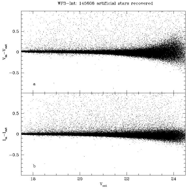
Figure 3: Differences between the input and output magnitudes of the artificial stars versus output $V$ magnitudes for the $V$ [panel (a)] and $I$ [panel (b] passbands, for the WF3int subfields shown as an exemple.

In Fig. 3 the differences between input magnitudes and output magnitudes are reported as a function of input magnitude for the artificial stars simulated and recovered in the WF3Int subfield, chosen as an example case (panel (a): $V_{\rm in}-V_{\rm out}$ vs $V_{\rm out}$, panel (b): $I_{\rm in}-I_{\rm out}$ vs $V_{\rm out}$). 182,441 stars were simulated in this case and 145,608 were recovered. The plots shows that our measures are very accurate: for instance, the average $\sigma(V_{\rm in}-V_{\rm out})$ and $\sigma(I_{\rm in}-I_{\rm out})$ are both $\leq 0.05$ mag in for $V_{\rm out}<23$.

The distributions of magnitude differences are not symmetrical: there is a almost uniform cloud of stars in the upper half of each plot that has no counterpart in the lower half region. These stars have been recovered with a significantly brighter magnitude than that assigned in input—they are the artificial stars that blended with a real stars of similar (or larger) brightness.

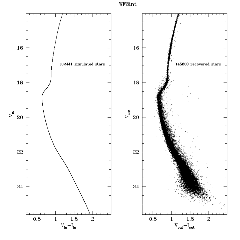
Figure 4: The CMD for the artificial stars obtained with input magnitudes (left panel) and output magnitudes (right panel). As an example, the results for the WF3int subfields are shown. The left diagram is mapped into the right diagram by the processes of observation and measure. Note the widening of the base of the RGB at $V>17$—this is the junction between the long and intermediate photometry. The stars just fainter than this limit are the highest S/N sources extracted from the long exposure frames, while the stars just brighter than this limit are lowest S/N sources of those extracted from the intermediate exposure frames. It is also interesting to note that the SMS is well populated by the numerous blendings occurred.

Fig. 4 shows the input (left panel) and output (right panel) CMD of the same set of artificial stars. Note the excellent agreement between the observed (Fig. 2) and simulated (Fig. 4, right panels) CMDs.

It is important to realize that the output CMDs demonstrate the effect of the observation and data reduction processes on the input stars, thus it can be thought as modeling a function that maps the true distribution of stars in the $(V,~{}V-I)$ plane into the observed version of the same distribution. Stars in the right panel of Fig. 4 have been subjected to all the effects that moved real stars from their true position in the $(V,~{}V-I)$ plane to their actually observed one.

Figure 5: Completeness factors as a function of $V$ magnitude for the 8 subfields.

As a check on the ability to recover stars of the whole procedure we show in Fig. 5 the completeness factors [$C_{f}=N_{\rm recovered}/N_{\rm added}$] as a function of $V$ for each of the eight subfields corresponding to the different chips of the Int and Ext fields. Note that the continuous line is not a fit to the data but is simply the line connecting them. The very low noise of the observed curves is a spin-off of the very large number of artificial star experiments performed. With the sole exception of the PC-Int subfield the completeness is quite similar everywhere and is larger than $80$ % at $V\leq 24$. The worse performance of the PC camera are mainly due to a brighter limiting magnitude at fixed $t_{\rm exp}$ with respect to WFs, because of the smaller pixel scale. We tested the possible crowding variation within each subfield by comparing the $C_{f}(V)$ curves obtained in different quadrants. In all cases the maximum quadrant to quadrant differences were $<2$–4% over the whole magnitude range. Thus, we concluded that the crowding conditions are very similar everywhere within each single subfield.

3 The Method

Our method for estimating $f_{b}$ is based on the comparison of the distributions of the color deviation from the Main Sequence Ridge Line (MSRL) of the real stars and of appropriate sets of artificial stars originally placed on the same MSRL. This is exactly as devised by RB97. We can imagine the effect of observation and data reduction on a stars as a sum of pulls that move it from the true place it would occupy in the CMD: photometric error provides a random pull while blending or the occurrence of a real binary system pulls the star systematically toward redder and brighter positions. The artificial star experiments optimally characterize the effects of photometric errors and blendings associated with the considered observation but do not include any pull due to the occurrence of a real binary. Thus, their distribution of color deviations from the MSRL should be different from that of a sample of real stars if binary systems are present. To estimate $f_{b}$, we produced additional artificial sets of MS artificial stars introducing a given fraction of binary systems, and then we compare the distribution of color deviations of the synthetic population to that of real stars, searching for the $f_{b}$ providing the best match to observations.

We apply the method to the MS in the range $20\leq V\leq 23$, were the SMS signal is most easily detected. For $V<20$ the MS is nearly vertical in the CMD and no significant color deviation can be detected. For $V>23$ the widening of the sequence due to photometric errors is too large to distinguish it from that introduced by a population of binary systems.

Figure 6: CMDs in the range $20\leq V\leq 23$ for (a) the sample of real stars observed into the WF2int subfield, (b) a synthetic catalog with $f_{b}=0$, (c) a synthetic catalog with $f_{b}=30\%$ and uniform $F(q)$ and (d) a synthetic catalog with $f_{b}=50\%$ and uniform $F(q)$. All the simulated CMDs contains the same number of stars as the observed sample and are extracted from the set of artificial stars simulated on the WF2int chip. Note that each of the simulations shown is just one of the infinite possible realizations of the CMD with the given $F(q)$ and $f_{b}$.

The general scheme adopted is the following:

1. Stars are randomly generated from an appropriate mass function. The associated $V$ magnitudes are obtained from an appropriate Mass vs. Luminosity relation obtained from theoretical isochrones. The corresponding $I$ magnitudes are obtained from the MSRL.

2. A given fraction of the generated stars is assumed to be the primary of a binary system; the secondary mass is assigned by randomly drawing from a mass ratio distribution $F(q)$. ¿From the extracted $q$ the mass and the $V$ and $I$ magnitudes are assigned to the secondary star, the $V$ and $I$ fluxes of the primary and secondary are summed and the final $V$ and $I$ magnitude of the unresolved binary system is obtained. The final product of this process is a list of $V$ and $I$ magnitudes, a fraction of which has been modified by the addition of the flux by a companion. The total number of entries of the list is equal to the size of the sample of real stars we have to compare with.

3. We associate to each entry in the list described above an artificial star having $V_{\rm in}$ within $\pm 0.03$ mag and that has been successfully recovered. Thus for each entry, either representing a single star or a binary system, we also obtain the corresponding $V_{\rm out}$ and $I_{\rm out}$ that takes into accounts all the possible pulls due to observational errors and eventual blendings. The final product is a list of synthetic stars with the same characteristics of the real stars, in which a known fraction of binary systems has been introduced. Note that each real star has a counterpart in the synthetic catalog which in turn has a final $V$ and $I$ from an artificial star that was recovered in the same region of the field were the real star is. Thus local variations of the crowding are taken into account and the whole process is done independently for each subfield. In Fig. 6 we show as an example, the CMD in the range $20\leq V\leq 23$ for (a) the WF2int sample of real stars, (b) a synthetic catalog with $f_{b}=0$, (c) a synthetic catalog with $f_{b}=30$ % and uniform $F(q)$ and (d) a synthetic catalog with $f_{b}=50$ % and uniform $F(q)$ (see caption for further details).

4. For each fixed $f_{b}$ and $F(q)$, 100 synthetic catalogs are generated. Each of these is one of the infinite number of possible random realizations of a sample having the same characteristics as the observed one and including a fraction of binary systems $f_{b}$ whose mass ratios are extracted from $F(q)$. The distribution of color deviations from the MSRL of each of these synthetic samples is compared to that of real stars by means of a function of merit and the average degree of agreement as well as the dispersion in the degree of agreement is finally determined.

5. The whole process is repeated for a wide grid of binary fractions and $F(q)$ distributions, and finally a probability curve as a function of $f_{b}$ is produced for each assumed $F(q)$ (cf., Fig. 6 of RB97).

We now examine in more detail some of the single steps.

3.1 The Mass Function

Since our original aims included placing constraints on the distribution of mass ratios, we preferred to produce our synthetic samples by extracting masses instead of luminosities or magnitudes, as done by RB97. Our tests showed that useful constraint on $F(q)$ from the SMS morphology can be derived only if the true binary fraction in the sample under consideration is larger than $30$ %. We adopted a Mass Generating Function (MGF) similar to that presented by Jarrod & Tout (1999), adjusted to fit the observed mass function of NGC 288. The MGF is just a numerical algorithm that maps random numbers between 0 and 1 into a given mass distribution, the relevant characteristic being its ability to reproduce a realistic distribution. In Fig. 7 the Luminosity Function (LF) derived from the adopted MGF (through a proper $M_{V}$ vs. Mass relation, described below) is compared to the completeness corrected LFs from the observed fields. In this case the samples from the WF cameras have been merged into the WF-Int and WF-Ext samples, while the PC-Int and PC-Ext LFs are shown separately. All the reported LFs have been normalized to approximately match each other in the range $18.5<V<20.5$. The LF from the Generating Function clearly provides a good representation of the observed LFs.

Figure 7: The LF derived from the Mass Generating Function (MGF; large full dots) compared to the completeness corrected LF for the PC-Int (open squares), the PC-Ext (open triangles), the combined WF-Ext cameras (open pentagons) and the WF-Ext cameras (open exagons). All the LF’s are normalized to approximately match in the range $18.5<V<20.5$. The MGF luminosity function is in good agreement with the observed ones.

To convert masses (in solar mass units) into $V$ magnitudes we utilized theoretical models. In particular, a $Z=0.002$ isochrone from the recent set by Cassisi et al. (2000) provides an excellent fit to the observations once corrected for distance and reddening [$(M-m)_{0}=14.73$ and $E(B-V)=0.03$, from Ferraro et al. (1999a)], as shown in Fig. 8. We use the fitted isochrone to derive the $Mass(V)$ function shown in Fig. 9, obtained by cubic spline interpolation.

Figure 8: Comparisons between the C2000 isochrone adopted to convert masses to $V$ magnitudes and the observations. In the left panel the isochrone (continuous line) is superposed to the observed CMD. In the right panel it is superposed to the MSRL (large open dots).

It should be noted that the only use of stellar models in the whole process is the conversion of extracted masses into $V$ magnitudes. Uncertainties intrinsic to the adopted model or associated with small errors in the fit would have some (moderate) impact only on the assumed $F(q)$ distributions. The actual $f_{b}$ estimates are based on color deviations from the MSRL and are largely independent from the assumed $Mass(V)$ function.

Figure 9: The adopted Mass - $V$ magnitude relation as derived from the theoretical isochrone presented in Fig. 8.

3.2 The Mass Ratio Distributions

Significant samples of local field binaries have been studied by various authors (Trimble, 1974; Trimble & Walker, 1986; Eggleton, Fitchett & Tout, 1989; Duquennoy & Mayor, 1991), reaching a reasonable agreement on the general form of the distribution of mass ratios $F(q)$. The local $F(q)$ shows a shallow peak at $q\sim 0.2$–0.3. The reality of a possible second peak at $q\sim 1$ has been questioned since it may be produced by selection effects. Tout (1991) has shown that, if all of the selection effects are taken into account, the observed $F(q)$ is naturally reproduced by extracting secondary stars from the observed Initial Mass Function, i.e. what would be expected by random associations between stars (hereafter we will refer to this kind of distribution as to the Natural $F(q)$).

There is neither observational constraint on the form of $F(q)$ in globular clusters, nor theoretical arguments suggesting that the original $F(q)$ in a globular has to be different from that of the field. However a difference in the formation of primordial binaries due to the higher environmental density cannot be excluded. On the other hand it is expected that a binary population in a globular may be subjected to significant evolution through (a) ionization of soft systems, (b) binary-single star and binary-binary interactions leading to star exchanges and, eventually, (c) tidal captures and/or merging of the two components (see Hut et al., 1992; Bailyn, 1995, and references therein). There is no reason to think that the processes leading to the disruption or merging of binary systems have some influence on $F(q)$, and the same conclusion is valid for the tidal capture phenomenon which is efficient only in extremely dense environments. Conversely, any exchange reaction would tend to preserve the most massive components in the bound system and to eject the lighter ones, thus moving mass ratios toward unity.

Given this framework, the only possible approach is to keep $F(q)$ as a sort of free parameter, by measuring $f_{b}$ under the assumption of different “toy models” for $F(q)$, as done by RB97. While in principle $0<q\leq 1$, this is not necessarily the case while dealing with the SMS technique, since there is a fundamental limit to the mass of secondary stars that can contribute additional flux to their primary, i.e., the stellar mass limit $M\sim 0.08M_{\odot}$. This limit, coupled with the maximum mass in the MS ($M\sim 0.8M_{\odot}$), sets a lower limit in the range of $q$. All of our model $F(q)$ include this limit to ensure that we remain in the star/star regime and avoid star/brown dwarf and star/planet systems.

In the choice of the possible $F(q)$ to adopt as test cases we have been driven by two obvious but opposite requirements, to cover the widest portion of the parameter space and to avoid an infinite amount of computing. Thus we considered toy models covering somewhat extreme cases with $F(q)$ peaking toward the extremes of the $q$ range, an intermediate one (uniform $F(q)$), and the most realistic model one can simply conceive, a natural distribution.

Fig. 10 shows the normalized histograms of 100,000 binary systems randomly drawn from each of the adopted $F(q)$ distributions. The lower limit $q>0.1037$ has been applied to each of them. The distribution Peaked at High Mass Ratios (PHMR; Fig. 10, panel b) has been produced with a generating function of the form $GF(q)=\sqrt{x}$, where $x$ is a random number within 0 and 1. For the distribution Peaked at Low Mass Ratios (PLMR; Fig. 10, panel c) with $GF(q)=1.-\sqrt{x}$ was adopted, The Natural distribution has been obtained by extracting the mass of both the primary and secondary component of the binary systems from the MGF.

RB97 modeled $F(q)$ through distributions of the $V$ magnitude ratio in the form $V_{2}=V_{1}/R^{\xi}$, where R is a random number between 0 and 1 and the exponent $\xi$ determines the form of the distribution. Six cases where considered, $\xi=0,~{}0.125,~{}0.250,~{}0.5,~{}1.0,~{}2.0$. The case $\xi=0$ is trivial (all binaries have $q=1$). The $F(q)$ associated with $\xi=0.125$ is very similar to our PHMR, while for $\xi=0.25$ $F(q)$ nearly corresponds to a uniform distribution. The cases $\xi=0.5,~{}1.0,~{}2.0$ all correspond to $F(q)$ peaked at low mass ratios, with different importance of the peaks. A lower limit to $q$ similar to ours was achieved by adopting a faint limit for the magnitude of the secondary. In the end, the range of mass ratio distributions sampled in the present analysis is similar to that considered by RB97.

Figure 10: Normalized histograms of 100,000 binary systems randomly drawn from the adopted $F(q)$ distributions. Panel a: uniform distribution; panel b: Peaked at High Mass Ratios (PHMR) distribution; panel c: Peaked at Low Mass Ratios (PLMR) distribution; panel d: Natural distribution. The limit $q>0.1037$ has been applied to all the distributions to exclude stars/brown dwarf systems from the estimate of the total binary fraction.

3.3 The Estimate of $f_{b}$

We compared the red sides of the $\Delta(V-I)$ distributions of each synthetic sample with the observed distributions by means of a Kolmogorov-Smirnov (KS) test as done by RB97. We sample the range of possible binary fractions at $5$ % steps i.e., $f_{b}=0.05,~{}0.10,~{}0.15,~{}0.20,...,~{}0.50$. RB97 adopted a $1$ % step. For each fixed $f_{b}$ and $F(q)$ we produced and compared 100 synthetic samples instead of 1000 as done by RB97. The latter two choices allowed a significant saving in computation time without any significant reduction of the accuracy of our estimates. In fact our tests demonstrated that in the present case (a), the $f_{b}$ with the highest probability of being compatible with the observation is easily picked out within the uncertainties with a $5$ % step, and for case (b) the mean probability associated with a $[f_{b},~{}F(q)]$ pair as estimated from 1000 simulations differs by negligible amounts from that estimated with 100 simulations.

3.4 Technical Comments

The present paper reports the final consequences of an extensive set of tests carried on to optimize the method and to try to extract all the possible information from the analysis of a well observed SMS. The results of such tests oriented our choices and drove us to a step by step definition of the final method. It is interesting to note that in many cases an alternative to an approach adopted by RB97 for some specific problem turned out to be unfruitful, forcing us to follow their path. This may indicate that the basic characteristics of the method are indeed best suited for the SMS technique. A detailed description of the many tests we have performed is beyond the scope of the present paper. We plan to present the most interesting results in another paper (Monaco et al., in preparation). However, there are several points worthy of comment here.

While it is valid to say that we adopted the RB97 method for the estimating the binary fraction, there are some differences in detail. For example, 1) we used a $Mass(V)$ function and 2) we adopted somewhat different $F(q)$. In the end, we felt it worthwhile to describe our method completely.

It is also important to note that the application of the method requires a very high accuracy in each step of the procedure. For instance, RB97 found small shifts in $\Delta(V-I)$ introduced by the artificial star experimental procedure. They were forced to adopt a MSRL for the artificial stars which was different from the observed MSRL. Despite of the different pipelines and reduction package used, the same problem occurred in our study. For our ‘fix’ we felt that it was a safer choice to adopt a different MSRL for each subset of artificial stars (i.e., PC-Int, WF2-Int, etc.). We verified that if the effect is ignored a significant fraction of the signal associated with the SMS is lost.

Furthermore, the final MSRLs of each set of artificial stars is based on $>50,000$ stars in the relevant range of magnitudes. Thus the derived MSRL is statistically a very robust representation of the mean locus of the artificial stars. This is not necessarily the case for the observed sample. While a robust MSRL can be derived for the total sample, tiny camera to camera differences in the photometry can be present, hence (a) the global MSRL may not be an optimal representation of the CMD of each single subfield and (b) the number of stars in each single subfield may not be sufficient to obtain a “local” MSRL sufficiently good for the present application. Since case (a) produces a small artificial (and symmetrical) widening of the observed $\Delta(V-I)$ distributions, fine adjustments are necessary to obtain consistent comparisons between observed and synthetic $\Delta(V-I)$. Otherwise, the relevant distorsion of the distributions (i.e., those associated with the red tail) would be smoothed by spurious global discrepancies. We regard this sensitivity to small inaccuracies as the major drawback of the SMS technique as developed by RB97 and in the present work. However, it is important to stress that if the described adjustments are neglected the fit to the observed data is worse but the final best fit $f_{b}$ estimate is unchanged.

4 The Binary Fraction of NGC288

In Fig. 11 [panel (a)] we compare the cumulative distributions of color deviations from the MSRL ($\Delta(V-I)_{MSRL}$) of the whole observed sample to a randomly extracted set of 70,000 artificial stars without any binary systems added (i.e., $f_{b}=0.0$). It is immediately evident that the observed distribution is significantly more skewed toward large color deviations. A KS test shows that the probability that the two distributions are extracted from the same parent population is significantly lower than $10^{-6}$. From this simple test, performing a direct comparison between observed and artificial stars, we obtain a first very important result: the observed distribution of $\Delta(V-I)_{MSRL}$ in NGC 288 cannot be produced by a stellar population made only of single stars, i.e., the binary fraction of the cluster is not null, $f_{b}>0.0$. Note that the same conclusion is obtained even if subsamples of artificial stars of the same size of the observed one are considered.

Since we have demonstrated that $f_{b}>0.0$ we can now turn to the actual determination of $f_{b}$. This goal is obtained through comparisons similar to that presented in panel (a) of Fig. 11. The observed sample is now compared with subsamples of artificial stars with varying fractions of binary systems added, according to the prescriptions described in §3 (see §3.3, in particular). One example of a good reproduction of the observed $\Delta(V-I)_{MSRL}$ distribution is shown in panel (b) of Fig. 11. This example was obtained assuming a binary fraction of $15$ % and a uniform $F(q)$. According to a KS test, the probability that the two compared distributions are drawn from the same parent population is $P=84$ %.

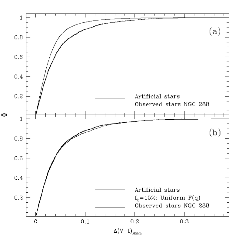
Figure 11: Panel (a): Comparison between the cumulative distributions of color deviations from the MSRL of the observed sample (thick line) and of a large subsample of artificial stars (thin line). The color deviations are only for stars in the range $20\leq V\leq 23$ (see §3.). Note that the observed distribution is significantly skewed toward larger color deviations with respect to the artificial star distribution that, by definition, contains no binaries. The probability that the compared samples are drawn from the same parent population is $P<10^{-6}\%$. Panel (b): a “good fit” case is also shown for comparison. The observed sample is compared to a realization of a synthetic sample of the same dimension with a binary fraction of $15\%$ drawn from a uniform distribution of mass ratios. The probability that the compared samples are drawn from the same parent population is $P=84\%$.

The results for all of the simulated samples are shown in Fig. 12. Each of the small dots (in the vertical columns) shows the probability that a given simulated sample is extracted from the same parent population of the observed sample as a function of the $f_{b}$ of the simulated sample. The different panels of Fig. 12 show the results obtained assuming different $F(q)$ (from top to bottom: PLMR, PHMR, Natural and Uniform). There are 100 of these for each $f_{b}$. The open circles give the average probability. The average points have been connected by a continuous line as an aid for the eye and as a first order interpolation between the obtained estimates.

Figure 12: Estimates of the binary fraction in the whole observed sample (Int+Ext), for the four $F(q)$ we considered. In each panel the probability that the actual simulated sample is drawn from the same parent population as the observed sample (according to a KS test) is plotted versus the binary fraction introduced in the simulated samples. Each small dot represents one of the 100 random realizations of the simulated sample at a given [$f_{b},F(q)$] pair. The open circles are the average probability of the 100 realizations of simulated samples. A line connecting the open circles has been drawn as an aid for the eye. The figure has been arranged in a way to be as similar as possible to the corresponding plots by RB97.

There are many features worthy of comment in Fig. 12:

1. Independently of the assumed $F(q)$, the observed distribution of color deviations is strongly incompatible with a binary fraction lower than $5$ %.

2. Compatibility with observations (at least marginal) can be obtained for 5 % $\leq f_{b}\leq 35$ %, depending of the adopted $F(q)$. However if we consider [$F(q),~{}f_{b}$] pairs which yield at least one case in which $P>1$ %, the compatibility with $f_{b}=5$ % remains only for the PHMR case, and even then for only one realization out of one hundred. On the other hand, the compatibility with $f_{b}=35$ % is excluded in all cases and $f_{b}=30$ % is only allowed for the PLMR. Hence, independently of the assumed $F(q)$, an appreciable compatibility (i.e., $P>1$ % in a non-negligible number of cases) is reached only for $5$ % $<f_{b}\leq 30$ %.

3. The most probable $f_{b}$ ranges from 10 to 20% depending on the assumed $F(q)$.

4. As expected the PLMR case provides both the highest $f_{b}$ estimate and the widest range of compatibility. This is because in this case most of the binaries are hidden near the MSRL and the observed SMS would be a minor component of the whole population.

5. The estimates obtained assuming a PHMR, Natural or Uniform distribution of mass ratios are rather similar. If these $F(q)$ are considered, the $P>1$ % compatibility range is $5$ % $<f_{b}\leq 20$ %.

The global field covers a significant fraction of the cluster within 2 $r_{h}$. Thus, we consider the above estimates as fairly representative of the whole population in NGC 288. Therefore, we conclude that the global binary fraction in NGC 288 is 5 % $\leq f_{b}\leq 30$ %, independently of the assumed $F(q)$, while recalling that the range giving the highest degree of compatibility with observations is $10\%\leq f_{b}\leq 20$ %. This result is in good agreement with the lower limit $f_{b}$ derived by Bolte (1992).

4.1 Radial Segregation

A very basic prediction of the theory of dynamical evolution of globular cluster is that such collisional systems tend to energy equipartition which in turn generates mass segregation. The heavier objects sink toward the central region of the system on timescales comparable with the relaxation time (Meylan & Heggie, 1997). The evolutionary rate driven by two-body encounters is quite low in NGC 288 because of its low stellar density. However, the cluster has an age comparable with the Hubble time ($\geq 10$ Gyr) which is much longer than its relaxation time (either central or median $t_{rc}\sim t_{rh}\sim 1$ Gyr; for either definitions and estimates see Djorgovski, 1993). Thus, the cluster should have dynamically relaxed long ago, and the binary systems, that are heavier than single stars in average, are expected to be significantly concentrated in the inner regions.

To verify this we considered separately the Int and Ext sample to provide an estimate of $f_{b}$ in the two regions at different radial distances from the cluster center. We take advantage of the lucky circumstance that, with good approximation, the Int field samples the region within $1r_{h}$ from the center, while the Ext samples the region between $1\,r_{h}$ and $2\,r_{h}$, so the comparison of the Int and Ext fields has a well defined physical meaning.

In principle, one might desire to divide the sample in many radial annuli, providing an estimate of $f_{b}$ in each annulus and obtaining a radial profile of the binary fraction. In practice, this approach turns out to be unviable because the method needs large samples to provide significant estimates (see also RB97), so each subdivision of the sample would reduce the constraining power of the test.

Figure 13: Estimates of the binary fraction in the Int sample, approximately enclosed in the region within 1 $r_{h}$ from the cluster center (see Fig. 1). The arrangement and symbols are the same as Fig. 12

Figure 14: Estimates of the binary fraction in the Ext sample, approximately enclosed in the region between 1 and 2 $r_{h}$ from the cluster center (see Fig. 1). The arrangement and symbols are the same as Fig. 12 and 13. Note that $f_{b}=0$ is by far the most likely binary fraction independently of the assumed $F(q)$.

In Fig. 13 the $f_{b}$ estimates for the Int region are presented. A direct comparison with Fig. 12 makes it immediately evident that the ranges of compatibility have shifted toward higher $f_{b}$ values, independently of the adopted $F(q)$. The results are no longer compatible with $f_{b}=5$ %. The broad range of compatibility is 8 % $<f_{b}\leq 38$ %, while the most probable $f_{b}$ values ranges from 10 % $to25$ %, depending on the $F(q)$ considered. These results suggest that the binary fraction within $1\,r_{h}$ is higher than in the global sample.

Fig. 14 shows the results obtained in the Ext region. Independently of the considered $F(q)$ the most probable binary fraction is 0 and in any case $f_{b}\leq$ 10 % ($P>1$ % compatibility range). Thus, there is a strong indication of a significant difference in binary fraction between the two considered radial zones. Furthermore, it can be concluded that most of the binary systems in NGC 288 reside within $1\,r_{h}$ from the cluster center, a clear effect of the mass segregation.

It is worth emphasizing that the above results cannot be achieved by a direct comparison of the $\Delta(V-I)_{MSRL}$ distributions of the Int and Ext samples, since they suffer from different degrees of crowding and, by consequence, have different photometric errors and rate of blending. It is expected that the stars in the Int sample have, on average, larger $\Delta(V-I)_{MSRL}$ with respect to the Ext ones. It was essential to determine if the difference induced by photometric errors and blendings was sufficient to explain the observed difference in the distribution of color deviations and to correctly quantify the effect of these factors. This was exactly the aim of the adopted technique, without which neither absolute nor differential $f_{b}$ estimates can be reliably obtained.

4.2 The Nature and Evolution of Binaries in NGC 288

Note that a binary fraction $f_{b}=10$ %, a value near the lower limit for the region within the half light radius, implies that 18 % of the cluster stars are bound in binary systems. Since the evolution of such stars may be somehow influenced by the presence of a companion, it is evident that a moderate binary fraction can have a significant impact on the production of anomalous populations in the cluster (BSS, sdB, etc).

With simple and basic theoretical arguments it is possible to derive some useful (though statistical in nature) constraints on the origin of the binary population of NGC 288. There are three possible origins for a binary in a globular cluster: (a) the member stars were gravitationally bound at their birth , i.e., the system is primordial, (b) occasionally three single stars can have a close encounter leaving two of them gravitationally bound, the third stars having gained the excess energy, i.e., a three body encounter, or (c) during a very close encounter, “two unbound stars can divert enough orbital energy in the form of stellar oscillation that the pair becomes bound” (Hut et al., 1992), i.e. a tidal capture.

According to Binney & Tremaine (1994) the number of binaries formed by three body encounters in a cluster having $N$ member stars is $\sim 0.1/(N\ln N)$ per relaxation time. The predicted number of such systems formed over the whole lifetime of NGC 288 is $\sim 10^{-7}$, under the very conservative assumption that all members have mass $1\,M_{\odot}$ and adopting the total mass estimate by Pryor & Meylan (1993), i.e. $M=10^{4.9}M_{\odot}$. The rate of tidal capture can be roughly estimated with the analytical formula provided by Lee & Ostriker (1986). Under the most conservative assumptions it turns out that the number of tidal captures that may have occurred in NGC 288 in its whole lifetime is $<10$. Thus, it can be concluded that the overwhelming majority of the binary systems in NGC 288 have a primordial origin.

Binary systems in a globular cluster may be broadly classified according to the ratio between their intrinsic energy and the typical kinetic energy of the cluster stars. Binaries are said to be hard or soft if their energy is, respectively, larger or lower than this value (Hut et al., 1992). As a general statistical rule, encounters between a single star and a binary results in an hardening for hard system (the unbound star is accelerated and the binary becomes more tightly bound) while soft binaries are softened (the unbound star is decelerated and the binary becomes less tightly bound; see Binney & Tremaine, 1994; Meylan & Heggie, 1997). The average result of the evolution driven by single star-binary encounters is that hard binaries increase their energy reservoir and decrease their cross section for close encounters, while soft binaries increase their cross section becoming less and less bound. Assuming an average mass of 0.2$\,M_{\odot}$ for the members of NGC 288, according to Kroupa (2001), it turns out that all of the binary systems formed by two MS stars and with semimajor axis larger than $\sim 5$ AU are soft. From eq. 8 of Hut et al. (1992) one finds that all of the primordial binaries with semimajor axis larger than $\sim 7$ AU are likely to have had at least one close encounter in their lifetime. Thus, it can be concluded that the population of soft binaries in NGC 288 has significantly evolved because of encounters with single stars, and probably most of the original soft binaries have been destroyed. Finally, if one considers only the population of hard binaries, neither binary-single star nor binary-binary encounters are expected to have had a large impact on the evolution of such systems.

To summarize these points:

• the population of binaries in NGC 288 is largely dominated by primordial systems;

• the present day population is likely to be mainly composed of hard binaries whose rate of evolution due to encounters is not great.

It has to be noted that the above conclusions are based on the hypothesis that the stellar density in NGC 288 was not significantly higher in the past. This possibility is shortly discussed in §5.3.1.

5 Blue Stragglers

Blue Straggler Stars (BSS) are hydrogen burning stars that presently have a mass higher than at their birth. This situation is thought to arise either via the collision and merger of two single stars (ss collision; a mechanism that may be efficient in the central regions of the densest globulars), or via the mass transfer and/or coalescence between the members of a binary system (see Stryker, 1993; Fusi Pecci et al., 1992; Bailyn, 1995; Mateo, 1996a; Sarajedini, 1997, and references therein). The coalescence between the members of a binary system may be favored by binary-binary encounters, an occurrence that greatly enhances the probability of a physical collision between two of the member stars (bb collision, see Leonard, 1989). While there are only indirect clues supporting the collisional scenario, the link between (at least some) BSS and binary systems is firmly established (Mateo, 1996b). However, it seems probable that either single star and binary mechanisms may be responsible of the formation of BSS in different conditions, even in different regions within the same cluster or at different epochs of the evolution of a cluster (see Fusi Pecci et al., 1992; Ferraro et al., 1993; Ferraro, Fusi Pecci & Bellazzini, 1995; Ferraro et al., 1997, 1999b; Sigurdsson, Davies & Bolte, 1994; Sills, 1998).

The presence of Blue Stragglers in NGC 288 was first noted by Alcaino & Liller (1980) and by Buonanno et al. (1984a, b). Bolte (1992) found a remarkable population of such stars and showed that BSS in NGC 288 are more centrally concentrated than SGB and RGB stars of comparable magnitude. This trend is observed in many other globulars and usually interpreted as due to the settling of the more massive BSS to the inner part of the clusters (however the interpretation of the radial distribution of BSS is not always so straighforward, see Ferraro et al., 1993; Bailyn, 1995).

5.0.1 BSS from binary-binary collisions in NGC 288

Before proceeding in the analysis, we estimate the efficiency of bb encounters in NGC 288 to check if this mechanism may be relevant for the production of BSS stars in this cluster (Leonard, 1989; Leonard & Fahlman, 1991).

According to Eq. 14 of Leonard (1989), adopting the structural and kinematical parameters from Djorgovski (1993, $r_{c}$) and Pryor & Meylan (1993, $M/M_{\odot},\sigma_{0}$), and assuming an average stellar mass of 0.2 $M_{\odot}$ as in §4.2 (Kroupa, 2001), the number of bb collisions per gyr ($N_{bb}$ [Gyr^-1]) in NGC 288 is:

$$N_{bb}\simeq 387.6af_{b}^{2}$$

where $a$ is the semimajor axis of the considered binaries in AU. If only hard binaries are taken into account ($a\leq 5$ AU; see §4.2) and a binary fraction $f_{b}=0.2$ is assumed (quite likely for the cluster core) $\sim 80$ bb collisions per gyr are expected. It is not clear how many of such encounters may ultimately lead to the physical collision between two members of the involved systems. However it is clear that bb encounters are a viable mechanism for the production of (at least) part of the BSS in NGC 288, unless the fraction of bb encounters producing a physical collision is significantly lower than ${1\over{100}}$.

5.1 BSS in the UV: Specific Frequency

A clear sequence of BSS is evident in the CMD of the Int sample in Fig. 1, while the Ext sample hosts at most one clear BSS candidate (see §5.2). We will discuss the radial distribution later on, since it is safer to assess the selection criteria of candidate BSS before. In Fig. 15 the BSS candidates are selected in the ($m_{F255W}$, $m_{F255W}-m_{F336W}$) CMD according to the criteria introduced by Ferraro et al. (1997, 1999b). In this plane the hottest sources are especially obvious and the BSS sequence stands out as an almost vertical plume at $16.50\leq m_{F255W}\leq 18.65$ and $-1.0\leq m_{F255W}-m_{F336W}\leq 0.4$. Furthermore, adopting this selection criterion allows a direct comparison with the clusters studied by Ferraro and collaborators (see Ferraro, 2000; Bellazzini & Messineo, 2000, and references therein). The F255W observations were available only for the Int field, thus the CMD presented in Fig. 1 refers to the region within $\sim 1\,r_{h}$ from the cluster center. The derived BSS specific frequency $F_{BSS}$, defined as the ratio between the number of BSS ($N_{BSS}$) and the number of HB stars ($N_{HB}$) observed in the same given field, is $F_{BSS}=1.35\pm 0.49$, where the error is the Poisson noise on the star counts. The specific frequency in the very central region $r\leq 1\,r_{c}$ is $F_{BSS}=1.45\pm 0.59$, while in the annulus $1r_{c}<r\leq 2r_{c}$ it is $F_{BSS}=1.00\pm 0.82$, hinting that the BSS population is more centrally concentrated than HB stars. It is very interesting to note that NGC 288 has a BSS frequency significantly higher than all the other clusters for which $F_{BSS}$ has been measured with this technique, i.e. M13, M3, M92, M30 all having $F_{BSS}\leq 0.67$ (see Table 1 in Bellazzini & Messineo, 2000, and references therein). The only exception is the core-collapsing cluster M80 in which Ferraro et al. (1999b) discovered an exceptionally abundant and extremely concentrated population of BSS (305 stars). M80 has a global frequency $F_{BSS}\simeq 1.0$, and $F_{BSS}\simeq 1.7$ in the core, very similar to NGC 288. Ferraro et al. (1999b) argued that during the phase of core collapse the extreme stellar density occurring in the core of M80 boosted the star-to-star collision rate, thus providing a very efficient mechanism for the production of collisional BSS. Since, as said, ss collisions are quite rare in the loose NGC 288, the observed exceptionally high specific frequency suggests that the formation of BSS via binary evolution in low density clusters can be as efficient as the ss collisional mechanism in very dense ones. The possible consequences of this result will be discussed in §6 (see also Renzini, Mengel & Sweigart, 1977; Nemec & Harris, 1987; Nemec & Cohen, 1989; Leonard, 1989; Leonard & Fahlman, 1991; Stryker, 1993).

Nearly at the center of Fig. 15, at $m_{F255W}\simeq 16.3$ and $m_{F255W}-m_{F336W}\simeq 0.6$, one can see a HB star much cooler than other stars in this phase. The same star stands out very clearly in the $(V,~{}V-I)$ CMD, at $V\simeq 15$ and $V-I\simeq 0.8$, in the panel (a) of Fig. 2. The position of this star in the CMD is consistent with the hypothesis that it is an Evolved BSS (E-BSS, see Ferraro et al., 1999b; Bellazzini & Messineo, 2000; Fusi Pecci et al., 1992), i.e. a BSS in its Helium burning phase.

Figure 15: Blue Stragglers selected in the ($m_{F255W}$, $m_{F255W}-m_{F336W}$) CMD. The F255W observations are available only for the Int field.

5.2 BSS in the $V,~{}V-I$ Plane

The selection criteria used above has been very useful in making strictly homogeneous comparisons with the BSS population of other clusters. However, to study the evolutionary status of our sample of BSS we must adopt a selection criterion, based on the ($V,~{}V-I$) CMD. Any such BSS sample may be somewhat contaminated by non-genuine BSS. In the vicinity of the upper MS and SGB sequences, blended stars and/or real detached binaries may be impossible to distinguish from bona fide BSS. For NGC 288, we can take advantage of our extensive set of realistic (with correct colors) artificial stars experiments to select a pure sample of BSS. In the panel (a) of Fig. 16 we show the CMD of a large ($\sim 200,000$ stars) randomly extracted subsample of artificial stars, in the region where the observed candidate BSS lie. The large number of artificial stars ensures that many blendings are included in the sample. Indeed, a number of stars are found outside the narrow band around the input ridge line. In particular, some blending between MS and SGB stars populates a small region to the blue of the SGB. We defined a selection box (the irregular polygon delimited by the thick line) as a region of the $V$, $V-I$ plane that is not contaminated by blended sources. Note that this approach is extremely conservative in avoiding spurious BSS. The number of stars found between the red edge of the selection box and the single-star SGB sequence is comparable in the artificial star CMD and in the observed one (Fig. 16, panel (b)), while the former sample is $\sim 25$ times larger than the observed sample. This means that most of the observed stars in that region of the CMD are genuine BSS or detached binary systems, and only a small minority must be attributed to blendings. (Note, for instance, the concentration of observed stars to the blue of the MSTO, between $V\simeq 18.8$ and $V\simeq 19.6$ and compare with the same region in the artificial star CMD). Still, we chose not to include these stars to ensure that the contamination by blendings and/or detached binaries is certainly null, and that our sample includes only bona fide BSS. This conservative approach causes us to lose roughly 20% of the potential BSS sample based on the fact that 28 out of the 35 UV selected BSS candidates in Fig. 15 also fall in the $V,~{}V-I$ selection box adopted here.

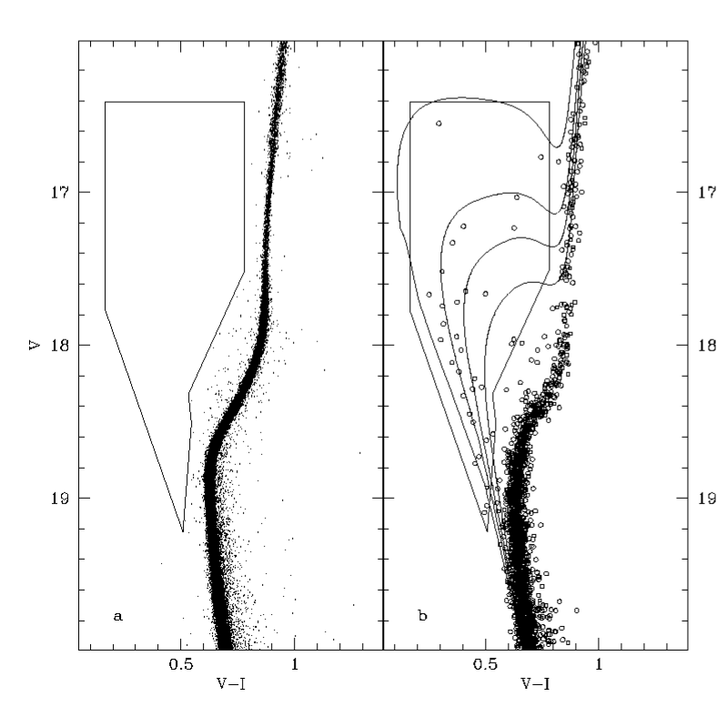
Figure 16: Blue Stragglers selected in the ($V$, $V-I$) CMD. Panel (a): $\sim 200,000$ artificial stars and the uncontaminated selection box (see text). Panel (b): the selection box is superimposed to the observed CMD (circles: stars of the Int sample; squares: stars of the Ext sample). Four isochrones ($Y=0.23$; $Z=10^{-3}$) from the set by Castellani, Degl’Innocenti & Marconi (1999). From left to right: Age = 2 Gyr, $M_{TO}=1.33\,M_{\odot}$; Age = 3.5 Gyr, $M_{TO}=1.13\,M_{\odot}$; Age = 4.5 Gyr, $M_{TO}=\,1.05M_{\odot}$; Age = 6 Gyr, $M_{TO}=0.96\,M_{\odot}$.

In the panel (a) of Fig. 16, the selection box is superimposed to the observed CMD (circles: Int sample; squares: Ext sample). The selected BSS sample contains 33 stars, just one of them belonging to the Ext sample

Four isochrones of the appropriate chemical composition ($Y=0.23$; $Z=10^{-3}$) from the set by Castellani, Degl’Innocenti & Marconi (1999) are also shown in the plot, assuming the reddening and distance modulus listed by Ferraro et al. (1999a). The faintest and reddest isochrone has an age of 6 Gyr, the mass of the stars at the TO is $M_{TO}=0.96\,M_{\odot}$; then, going toward bluer color and younger ages, age = 4.5 Gyr, $M_{TO}=\,1.05\,M_{\odot}$; age = 3.5 Gyr, $M_{TO}=\,1.13M_{\odot}$; and finally age = 2 Gyr, $M_{TO}=1.33\,M_{\odot}$. The reported isochrones encompass the whole distribution of BSS, thus constraining the range of masses covered by the selected BSS to $0.9\,M_{\odot}\leq M_{BSS}\leq 1.4\,M_{\odot}$. Blue Stragglers with $M_{BSS}\leq 0.8\,M_{\odot}$, i.e. formed by the merging of low mass MS stars, are still hidden in the single-star Main Sequence.

There are some BSS that cannot lie on the MS of any reasonable isochrone (at $V<17.4$ and $V-I>0.6$), but which can be well fitted by the SGB sequences. Given our stringent selection criteria, there may be very little doubt that these stars have evolved to the thinning hydrogen burning shell phase and are rapidly moving to the base of the RGB, i.e., they are Yellow Stragglers (YS; Hut et al., 1992; Portegies Zwart, Hut & Verbunt, 1997a; Portegies Zwart et al., 1997b).

5.3 Evolution of the BSS

5.3.1 The Conventional Merger Scenario and BSS Formation Rate

Most modern BSS formation scenarios have the implicit hypothesis that there is no preferred mass ratio for the stars that merge to form a new BSS. For instance, in the simulations by Sills & Bailyn (1999); Sills et al. (2000) the merging stars are drawn at random from a properly choosen IMF of single stars. Furthermore, Sills’ models assume that all BSS are the final result of a merging between two stars. Given this, simple considerations about the stellar lifetimes predict that if the rate of formation of BSS were constant over the lifetime of a globular, or at least from a given epoch in the past to the present day, the number of observed BSS must increase toward the red-faint part of the sequence, i.e., near the single-star MS and SGB. The prediction is quantitatively confirmed by detailed models of BSS populations (Sills, 1998; Sills & Bailyn, 1999; Sills et al., 2000). This is certainly not the case of NGC 288. Even in the region between the 2 Gyr and the 6 Gyr isochrones the number of BSS decreases toward the redder-fainter direction. There are 13 BSS between the 2 Gyr and the 3.5 Gyr isochrones, 9 between the 3.5 Gyr and 4.5 Gyr isochrones and 5 between the 4.5 Gyr and 6 Gyr isochrones. Taking the counts between 2 Gyr and the 3.5 Gyr isochrones as normalization point and assuming uniform rate of BSS production, crude estimates based on lifetimes would predict $\sim 19$ BSS in the region between the 3.5 Gyr and 4.5 Gyr isochrones and $\sim 24$ between the 4.5 Gyr and 6 Gyr isochrones. It can be concluded that the observed distribution of BSS in the CMD is not consistent with a constant rate of production over a long time ($\sim 5$ Gyr or larger).

The BSS in our sample lie in a remarkably narrow band, significantly clustered around the 3.5 Gyr isochrone. Indeed, the observed distribution of BSS in NGC 288 resembles that predicted by BSS evolutionary models with a short 1–2 Gyr burst of BSS formation which occurred 1–4 Gyr ago, (see in particular Fig. 1 and Fig. 3 of Sills et al., 2000).

A BSS formation rate with significant variations with time has been recently invoked to explain the BSS distribution in M80 (Ferraro et al., 1999b) and in 47 Tuc (Sills et al., 2000). A possible explanation for the enhancement of the BSS production rate that appear to have occured in NGC 288 may be related to the process of mass segregation that, during the lifetime of the cluster, has collected more and more binaries in the cluster core, thus enhancing the rate of bb collisions. However, according to the present day relaxation time, the segregation of binaries into the cluster core should have occurred long time ago, at most a few $t_{rh}\sim 1$ gyr after the birth of the cluster.

The conclusion that phenomena driven by collisions are highly inefficient in NGC 288 (§4.2.) has been drawn on the basis of the presently observed structural and dynamical conditions of this cluster. However such conditions may have been different in the past. It may be conceived that NGC 288 was significantly denser in the past and has been brought to the present status by the disruptive effects of disc and bulge shocks. If this were the case, it can be imagined that the peak of BSS production rate coincided with the epoch of maximum contraction of the cluster, during which BSS may have been efficiently produced by stellar collisions. The subsequent expansion decreased the collision rate to the present level, virtually stopping the production of collisional BSS.

While this framework provide an explanation for the deduced variation of the BSS formation rate with time, there are reasons to regard it as unlikely. In fact, to raise the collision rate at the required level it would have been necessary for NGC 288 to reach central densities some 100 - 1000 times larger than the present one. Since shocks fasten the internal evolution, the cluster would probably reach the core collapse phase (Meylan & Heggie, 1997; Gnedin & Ostriker, 1997). Even if binaries stopped the collapse, it would be very difficult to re-expand the cluster core to the present status. While most of the cluster halo may have been torn apart in the subsequent perigalactic passages, the dense core would have become very resistent to shocks. Thus the cluster present-day density would have been sinificantly higher than observed. On the other hand, if the cluster experienced a shock so strong to alter its whole structure, this would finally lead to its complete disruption. Since from its birth NGC 288 had $\sim 50$ perigalactic passages, probably it would have not survived to the present day.

5.3.2 An Alternative View: Evolutionary Mass Transfer

Let’s consider now the alternative hypothesis that the BSS population in NGC 288 is dominated by stars that increased their original mass via mass transfer from their primary (McCrea, 1964; Collier & Jenkins, 1984, hereafter CJ84).

In this case the rate of formation of BSS will be driven by the rate that stars leave the main sequence. At the age of NGC 288 0.8$\,M_{\odot}$ stars leave the main sequence and might begin to transfer mass on the lower RGB. They might dump most of their mass down to some helium core, say 0.2$\,M_{\odot}$, onto the secondary. If $F(q)$ is peaked for large $q$, say 0.6–1.0, then the resulting star will have a mass 1.08–1.40$\,M_{\odot}$. Even for a natural $F(q)$ only 18% of binaries have $q<0.4$ so 82% of BSS would have $M>0.92$$\,M_{\odot}$. As the mass of the secondary increases the Roche lobe moves toward the primary. Mass transfer will take place more easily. Indeed stable mass transfer can occur only in binary systems with mass ratio not too far from unity. For example CJ84 assume a critical mass ratio $q_{\rm crit}\geq 0.4$ as the condition for stable mass transfer. With this condition, the lowest possible mass for a present day forming BS in NGC 288 would be 0.92$\,M_{\odot}$.

In the scenario described above there is a strict lower limit for the mass of a BSS and the formation of more massive BSS is clearly promoted. In this case the observed BSS distribution may be accomodated with a rate of production running at a pace set by the evolutionary rate of cluster stars (e.g., see the predicted BSS distribution in Fig. 2g by CJ84). It is interesting to note that in the CJ84 model (# 12) that is most like a typical globular cluster, a high specific frequency of BSS is (crudely) predicted, $F_{BSS}\sim 2.5$ within a factor 2 of what observed in NGC 288. Note that CJ84 assumed empirically-determined distributions of binary orbital periods and mass ratios, thus the fraction of mass-transfer systems producing BSS was not artificially boosted.

The framework depicted above seems to provide a natural explanation for the observed properties of the BSS population in NGC 288 without invoking a burst of BSS formation. Still it is clear that understanding the NGC 288 BSS population requires more work. Spectroscopic follow-up of individual BSS might help to distinguish between different scenarios, though the spectral signatures of the various possible origins are also not well defined (Stryker, 1993; Bailyn, 1995; Sills, 1998).

6 Summary and Discussion

We have measured the fraction of binary system ($f_{b}$) in the loose globular cluster NGC 288 using the SMS method to identify binaries in the $V,~{}V-I$ CMD. We employed a technique that accurately accounts for all the observational effects (observational scatter, blending, etc., see RB97) that may affect the estimate of $f_{b}$. This is only the second measurement of this kind ever obtained for a globular cluster, the first having been made by RB97 for NGC 6752.

We find that the observations are strongly incompatible with the hypothesis $f_{b}=0$ %, independently of any assumption concerning the distribution of mass ratios, $F(q)$, thus the presence of binary systems in NGC 288 is confirmed beyond any doubt (see also Bolte, 1992). We have estimated $f_{b}$ for various assumed $F(q)$, and have found that, independently of the adopted $F(q)$, the observations are strongly incompatible with global binary fractions lower than 5–7% or higher than $\sim 30$ %.

The binary fraction in the region within the half-light radius ($r_{h}$) is significantly larger than in the region outside this limit. For $r<1\,r_{h}$, 8 % $<f_{b}\leq 38$ % and the most probable binary fractions ranges from 10 % to 25 %, depending somewhat on the assumed $F(q)$. On the other hand, for $r>1\,r_{h}$, $f_{b}\leq 10$% and the most probable binary fraction is $f_{b}=0$ %, independently of the assumed $F(q)$. Hence, binary systems are much more abundant in the inner regions of the cluster, a clear sign of the occurrence of dynamical mass segregation.

Simple dynamical arguments strongly suggest that the large majority of binary systems present in NGC 288 are of primordial origin, and that single star - single star collision processes are highly inefficient in this cluster. Thus the large majority of the BSS in NGC 288 must have a binary origin. Despite that, NGC 288 has a very high Specific Frequency of BSS, comparable to or exceeding that of much more dense clusters. Like the binaries, the BSS population is centrally concentrated with virtually all the identified BSS lie within $1\,r_{h}$ from the cluster center.

The selected BSS candidates appear to have masses between $\sim 0.9M_{\odot}$ and $\sim 1.4M_{\odot}$, and form a remarkably narrow and well defined sequence in the $(V,~{}V-I)$ CMD. If the majority of BSS have been produced by the merging of two binary member stars, then the BSS distribution is not compatible with a BSS formation rate which has been constant in time. On the contrary, the existence of a significant peak in the BSS formation rate in the recent past ($\sim 1$–4 Gyr ago and lasting $\sim 1$–2 Gyr) is suggested by the comparison with theoretical models (Sills et al., 2000). The observations also seem compatible with a scenario in which most of the BSS population of NGC 288 has been producted via the mass transfer occurring in close binary systems.

A few yellow stragglers and one candidate E-BSS (in the Helium burning phase) have also been identified.

6.1 Binary Fraction: Comparisons with Other Systems

The two globular clusters for which a robust estimates of the global binary fraction have been obtained using the SMS technique, i.e., NGC 6752 (RB97) and NGC 288 (this work) are very different in terms of stellar density. The central density in NGC 6752 is $\sim 1000$ times that of NGC 288. It is very likely that the past dynamical evolution of the two clusters has been very different. Despite of that, the present day observed binary fraction (and binary distribution) is remarkably similar, at least at the present level of accuracy. However, while many details of the radial distribution of the binary populations are beyond the reach of the present day techniques, a first comparison of their broad properties is now possible. For NGC 6752 $15\%\leq f_{b}\leq 38\%$ within $1\,r_{c}$ from the cluster center and $f_{b}\leq 16\%$ in the outer region. For NGC 288 8 % $\leq f_{b}\leq 38$ % within $1\,r_{h}\simeq 1.6\,r_{c}$ and $f_{b}\leq 10$ % in the outer region. It may be presumed that a broad upper limit is set by primordial conditions and by the fact that in any globular cluster a significant number of binaries are soft (and thus are rapidly destroyed). Lower limits may be set by the equilibrium between destruction and formation of binary systems, somehow regulated by the density of the environment (since the efficiency of both mechanisms increase with stellar density, Hut et al., 1992).

It is also interesting to note that the global $f_{b}$ extrapolated from spectroscopic binaries and/or eclipsing variable searches in globulars is broadly constrained to be in the range 10 % $\leq f_{b}\leq 40$ % (see Mateo, 1996a, and references therein). Hence, two decades after the pioneering (and negative) results by Gunn & Griffin (1979), a very different picture of binaries in globular clusters seems firmly established: the binary fraction in globulars is not null (and likely larger than $\sim 5-10$ %), but is still significantly lower than in most of other environments, i.e., the local field, open clusters and star forming regions, for which $f_{b}\geq 50$ % (Mateo, 1996a; Mathieu, 1996; Duquennoy & Mayor, 1991).

6.2 Blue Stragglers in Low Density Systems

One of the most interesting results of the present analysis is the demonstration that the formation of BSS via mass transfer/coalescence of primordial binary systems may be as efficient as collisional mechanisms, occurring in the most favorable environments (see §5). This is a further (and quantitative) piece of evidence indicating that large populations of BSS may be produced in environments with remarkably low stellar density, if a sufficient reservoir of primordial binaries is available (see also Nemec & Harris, 1987; Nemec & Cohen, 1989; Leonard & Linnell, 1992; Leonard, 1993; Mateo, 1996a, b, and references therein).

This statement may have important consequences in the interpretation of the ubiquitous “blue plumes” observed above the main MSTO in the CMD of many dwarf Spheroidal galaxies (dSphs) dominated by old “globular-cluster-like” populations (as for instance Ursa Minor, Draco, Sextans and Sagittarius, see Martínez-Delgado et al., 2001; Carney & Seitzer, 1986; Mateo et al., 1991; Bellazzini, Ferraro & Buonanno, 1999, respectively, and references therein). These sparsely populated sequences are usually associated with recent, very small episodes of star formation. This hypothesis is also supported by the presence of stellar species thought to result from the evolution of stars with initial mass larger than the typical TO mass of old population (1–$2\,M_{\odot}$ vs. $0.8\,M_{\odot}$), such as Anomalous Cepheids (AC) and/or bright AGB stars (see Mateo, 1998; Da Costa, 1998, and references therein). Even though the blue plumes lie in the region of the CMD populated by BSS, BSS are sometimes considered an unlikely explanation because of the very low density environments.

The results presented here confirms that a dense environment is not a conditio sine qua non for the efficient production of BSS. Further, there is no reason to believe that primordial binaries are under-abundant in dSphs (see also Leonard & Fahlman, 1991; Leonard, 1993, and references therein). Indeed, the few available estimates suggest that (at least in Ursa Minor and Draco) the binary fraction may be even larger than in the local field (Olszewski, Pryor & Armandroff, 1996). It is also important to recall that once a star more massive than the typical old TO stars is formed from a binary system (via mass transfer or coalescence), it will follow the evolutionary path typical of its new mass, thus possibly passing through the AC or bright-AGB phases (as succesfully demonstrated by Renzini, Mengel & Sweigart, 1977, more than two decades ago). There is every reason to suspect a significant BSS population in dSphs, and they remain a viable explanation for the blue plumes (see, e.g. Grillmair et al., 1998).

Table 1: Observational material.

Field	Filter	$t_{exp}$ [s]	N
Int	F814W	140	4
Int	F814W	12	2
Int	F814W	1.2	1
Int	F555W	100	4
Int	F555W	14	2
Int	F555W	2.3	1
Int	F336W	1700	1
Int	F336W	1000	2
Int	F336W	60	1
Int	F255W	350	2
Ext	F814W	160	3
Ext	F814W	40	1
Ext	F555W	230	2
Ext	F555W	200	1
Ext	F555W	40	1

Note. — The fourth column (N) reports the number of repeated exposures taken in a given passband.

References

- Alcaino & Liller (1980) Alcaino, G., & Liller, W., 1980, AJ, 85, 1592
- Bailyn (1995) Bailyn, C. D., 1995, ARA&A, 33, 133
- Bellazzini, Ferraro & Buonanno (1999) Bellazzini, M., Ferraro, F.R., & Buonanno R., 1999, MNRAS, 307, 619
- Bellazzini & Messineo (2000) Bellazzini, M., & Messineo, M., 2000, in The Evolution of the Milky Way: Stars versus Clusters, F. Matteucci and F. Giovannelli Eds., Dordrecht, Kluwer, Astroph. & Sp. Science, 255, 213
- Bellazzini et al. (2001) Bellazzini, M., Fusi Pecci, F., Ferraro, F.R., Galleti, S., Catelan, M., & Landsman, W.B., 2001, AJ, in press
- Bergbusch (1993) Bergbusch, P.A., 1993, AJ, 106, 1024
- Binney & Tremaine (1994) Binney, J., & Tremaine, S., 1994, Galactic Dynamics, Princeton (NJ), Princeton University Press
- Bolte (1992) Bolte, M., 1992, ApJS, 82, 145
- Buonanno et al. (1984a) Buonanno, R., Corsi, C.E., Fusi Pecci, F., Alcaino, G., & Liller, W., 1984, A&AS,57, 75
- Buonanno et al. (1984b) Buonanno, R., Corsi, C.E., Fusi Pecci, F., Alcaino, G., & Liller, W., 1984b, ApJ, 227, 220
- Carney & Seitzer (1986) Carney, B. W., & Seitzer, P., 1986, AJ, 92, 23
- Cassisi et al. (2000) Cassisi, S., Castellani, V., Ciarcelluti, P., Piotto, G., & Zoccali, M., 2000, MNRAS, 315, 679 (C2000)
- Castellani & Castellani (1993) Castellani, M., & Castellani, V., 1993, ApJ, 407, 649
- Castellani, Degl’Innocenti & Marconi (1999) Castellani, V., Degl’Innocenti S., & Marconi, M., 1999, MNRAS, 303, 265
- Collier & Jenkins (1984) Collier, A.C., & Jenkins, C.R., 1984, MNRAS, 211, 391 [CJ84]
- Da Costa (1998) Da Costa, G. S., 1998, in Stellar astrophysics for the local group : VIII Canary Islands Winter School of Astrophysics, A. Aparicio, A. Herrero, and F. Sanchez Eds., Cambridge - New York, Cambridge University Press, p.351
- Dolphin (2000a) Dolphin, A.E., 2000, PASP, 112, 1383
- Dolphin (2000b) Dolphin, A.E., 2000, PASP, 112, 1397
- Djorgovski (1993) Djorgovski, S.G., 1993, in Structure and Dynamics of Globular Clusters, S.G. Djorgovski and G. Meylan eds., ASP, S. Francisco, ASP Conf. Ser., vol. 50, p. 373
- Duquennoy & Mayor (1991) Duquennoy, A., & Mayor, M., 1991, A&A, 248, 485
- Eggleton, Fitchett & Tout (1989) Eggleton, P.P., Fitchett, M.J., & Tout, C.A., 1989, ApJ, 347, 998
- Ferraro et al. (1993) Ferraro, F.R., Fusi Pecci, F., Cacciari, C., Corsi, C.E., Buonanno, R., Fahlman, G.G., & Richer, H.B., 1993, AJ, 106, 2324
- Ferraro, Fusi Pecci & Bellazzini (1995) Ferraro, F.R., Fusi Pecci, F., & Bellazzini, M., 1995, A&A, 194, 80
- Ferraro et al. (1997) Ferraro, F.R., et al., 1997, A&A, 324, 915
- Ferraro et al. (1999a) Ferraro, F.R., Messineo, M., Fusi Pecci, F., Straniero, O., Chieffi, A., & Limongi, M., 1999a, AJ, 118, 1758
- Ferraro et al. (1999b) Ferraro, F.R., Paltrinieri, B., Rood, R.T., & Dorman, B., 1999b, ApJ, 522, 983
- Ferraro (2000) Ferraro, F.R., 2000, in The Evolution of the Milky Way: Stars versus Clusters, F. Matteucci and F. Giovannelli Eds., Dordrecht, Kluwer, Astroph. and Sp. Science, 255, 205
- Fusi Pecci et al. (1992) Fusi Pecci, F., Ferraro, F.R., Corsi, C.E., Cacciari, C., & Buonanno, R., 1992, AJ, 104, 1831
- Gnedin & Ostriker (1997) Gnedin, O. Y., & Ostriker, J. P., 1997, ApJ, 474, 223
- Green (2001) Green, E.M., 2001, in Joint European and National Meeting JENAM 2001 of the European Astronomical Society and the Astronomische Gesellschaft, Astronomische Gesellschaft Abstract Series, Vol. 18., # MS 09 11
- Green, Liebert, & Saffer (2001) Green, E. M, Liebert, J., & Saffer, R. A. 2001, in Twelfth European Workshop on White Dwarfs (San Francisco:ASP), in press (astro-ph/0012246)
- Grillmair et al. (1998) Grillmair, C.J., et al., 1998, AJ, 115, 144
- Gunn & Griffin (1979) Gunn, J. E., & Griffin, R. F., 1979, AJ, 84,752
- Holtzman et al. (1995) Holtzman J.A., Burrows C.J., Casertano S., Hester J.J., Trauger J.T., Watson A.M., & Worthey G., 1995, PASP, 107, 1065
- Hurley & Tout (1998) Hurley, J., & Tout, C. A., 1998, MNRAS, 300, 977
- Hut et al. (1992) Hut, P., McMillan, S., Goodman, J., Mateo, M., Phinney, E.S., Pryor, C., Richer, H.B., Verbunt, F., & Weinberg, M., 1992, PASP, 104, 981 [HAL92]
- Irwin & Trimble (1984) Irwin, M.J., & Trimble, V., 1984, AJ, 89, 83
- Jarrod & Tout (1999) Jarrod, H., & Tout, C.A., 1999, MNRAS, 300, 977
- Kroupa (2001) Kroupa, P., 2001, MNRAS, 322, 231
- Latham (1996) Latham, D. W.,1996, in The Origins, Evolution, and Destinies of Binary Stars in Clusters, E.F. Milone and J.C. Mermilliod eds., ASP, S. Francisco, ASP Conf. Ser., vol. 90, p. 31
- Lee & Ostriker (1986) Lee, H-M., & Ostriker, J., 1986, ApJ, 310, 176
- Leonard (1989) Leonard, P.J.T., 1989, AJ, 98, 217
- Leonard & Fahlman (1991) Leonard, P.J.T., & Fahlman, G.G., 1991, AJ, 102, 994
- Leonard & Linnell (1992) Leonard, P.J.T., Linnell, A.P., 1992, AJ, 103, 1928
- Leonard (1993) Leonard, P.J.T. 1993, in Blue Stragglers, R.E. Saffer ed., ASP, S. Francisco, ASP Conf. Ser., vol. 53, p. 186
- Martínez-Delgado et al. (2001) Martínez-Delgado, D., Alonso-Garcìa, J., Aparicio, A., & Gòmez-Flechoso, M. A., ApJ, 459, L63
- Mathieu (1996) Mathieu, R. D., 1996, in The Origins, Evolutions, andcDestinies of Binary Stars in Clusters, E.F. Milone and J.C. Mermilliod eds., ASP, S. Francisco, ASP Conf. Ser., vol. 90, p. 231
- Mateo et al. (1991) Mateo, M., Nemec, J., Irwin, M., & McMahon, R., 1991, AJ, 101, 1102
- Mateo (1996a) Mateo, M., 1996a, in The Origins, Evolutions, and Destinies of Binary Stars in Clusters, E.F. Milone and J.C. Mermilliod eds., ASP, S. Francisco, ASP Conf. Ser., vol. 90, p. 21
- Mateo (1996b) Mateo, M., 1996b, in The Origins, Evolutions, and Destinies of Binary Stars in Clusters, E.F. Milone and J.C. Mermilliod eds., ASP, S. Francisco, ASP Conf. Ser., vol. 90, p. 346
- Mateo (1998) Mateo, M., 1998, ARA&A, 36, 435
- Maxted et al. (2001) Maxted, P. F. L., Heber, U., Marsh, T. R., & North, R. C. 2001, MNRAS, in press (astro-ph/0103342)
- McClure et al. (1985) McClure, R.D., Hesser, J.E., Stetson, P.B., & Stryker, L.L., 1985, PASP, 97, 665
- McCrea (1964) McCrea, W.H., 1964, MNRAS, 128, 147
- Meylan & Heggie (1997) Meylan, G., & Heggie, D. C., 1997, A&A Rev., 8, 1
- Nemec & Harris (1987) Nemec, J.M., & Harris, H.C., 1987, ApJ, 316, 172
- Nemec & Cohen (1989) Nemec, J.M., & Cohen, J.G., 1989, ApJ, 336, 780
- Olsen et al. (1998) Olsen K.A.G., Hodge P.W., Mateo M., Olszewski E.W., Schommer R.A., Suntzeff N.B., & Walker A.R., 1998, MNRAS, 300, 665
- Olszewski, Pryor & Armandroff (1996) Olszewski, E. W., Pryor, C., & Armandroff, T. E., 1996, AJ, 111, 750
- Piotto & Zoccali (2000) Piotto, G., & Zoccali, M., 2000, A&A, 358, 943
- Portegies Zwart, Hut & Verbunt (1997a) Portegies Zwart, S. F., Hut, P., & Verbunt, F., 1997a, A&A, 328, 143
- Portegies Zwart et al. (1997b) Portegies Zwart, S. F., Hut, P., McMillan, S. L. W.,&, Verbunt, F., 1997b, A&A, 328, 143
- Portegies Zwart, Yungelson & Nelemans (2000) Portegies Zwart, S. F., Yungelson, L. R., & Nelemans, G., 2000, in The Formation of Binary Stars, IAU Symp. n. 200, H. Zinnecker and R. Mathieu eds., ASP, S. Francisco, in press (astro-ph/0008033)
- Pryor & Meylan (1993) Pryor, C., & Meylan, G., 1993, in Structure and Dynamics of Globular Clusters, S.G. Djorgovski and G. Meylan eds., ASP, S. Francisco, ASP Conf. Ser., vol. 50, p. 357
- Renzini, Mengel & Sweigart (1977) Renzini, A., Mengel, J. G., & Sweigart, A. V., 1977, A&A, 56, 369
- Romani & Weinberg (1991) Romani, R. W., & Weinberg, M. D., 1991, ApJ, 372, 487
- Rosenberg et al. (2000) Rosenberg A., Piotto G., Saviane I., & Aparicio A., 2000, A&AS, 144,5
- Rubenstein & Bailyn (1997) Rubenstein, E. P., & Bailyn, C. D., 1997, ApJ, 474, 701 (RB97)
- Saffer, Green & Bowers (2001) Saffer, R. A., Green, E. M., & Bowers, T. P. 2001, in Twelfth European Workshop on White Dwarfs (San Francisco: ASP), in press (astro-ph/0012244)
- Sarajedini (1997) Sarajedini, A., 1997, in The Third Conference on Faint Blue Stars, A. G. D. Philip, J. Liebert, R. Saffer and D. S. Hayes Eds., Schenectady (NY): L. Davis press, p. 153
- Schechter, Mateo & Saha (1993) Schechter P., Mateo M., & Saha A., 1993, PASP, 105, 1342
- Sigurdsson, Davies & Bolte (1994) Sigurdsson, S., Davies, M.B., & Bolte, M., 1994, ApJ, 431, L115
- Sills (1998) Sills, A.I., 1998, Ph.D. Thesis, Yale University
- Sills & Bailyn (1999) Sills, A.I., & Bailyn, C.D., 1999, 513, 428
- Sills et al. (2000) Sills, A.I., Bailyn, C.D., Edmonds, P.D., & Gilliland, R.L., 2000, ApJ, 535, 298
- Spitzer (1987) Spitzer, L., 1987, Dynamical Evolution of Globular Clusters, Princeton (NJ), Princeton University Press
- Stryker (1993) Stryker, L.L., 1993, PASP, 105, 1081
- Tout (1991) Tout, C.A., 1991, MNRAS, 250, 701
- Tosi et al. (2001) Tosi, M., Sabbi, E., Bellazzini, M., Aloisi, A., Greggio, L., Leitherer, C., & Montegriffo, P., 2001, AJ, in press (astro-ph/)
- Trager, Djorgovski & King (1993) Trager, S.C., Djorgovski, S.G., & King, I.R., 1993, in Structure and Dynamics of Globular Clusters, S.G. Djorgovski and G. Meylan eds., ASP, S. Francisco, ASP Conf. Ser., vol. 50, p. 347
- Trimble (1974) Trimble, V., 1974, AJ, 79, 967
- Trimble & Walker (1986) Trimble, V., & Walker, D., 1986, Astr. & Space Sci., 126, 243
- Veronesi et al. (1996) Veronesi, C., Zaggia, S., Piotto, G., Ferraro, F.R., & Bellazzini, M., 1996, in Formation of the Galactic Halo … Inside and Out, H. Morrison and A. Sarajedini eds., ASP, S. Francisco, ASP Conf. Ser., vol. 92, p. 301
- Webbink (1985) Webbink, R., 1985, in Dynamics of Star Clusters, IAU Symp. n. 113, J.Goodman and P. Hut Eds., Dordrecht: Reidel, p. 541
- Whitmore, Heyer & Casertano (1999) Whitmore, B., Heyer, I., & Casertano S., 1999, PASP, 111, 1559