A scaling law for interstellar depletions

Abstract

An analytical expression is presented that allows gas-to-dust elemental depletions to be estimated in interstellar environments of different types, including Damped Ly $\alpha$ systems, by scaling an arbitrary depletion pattern chosen as a reference. As an improvement on previous work, the scaling relation allows the dust chemical composition to vary and includes a set of parameters which describe how sensitive the dust composition is to changes in both the dust-to-metals ratio and the composition of the medium. These parameters can be estimated empirically from studies of Galactic and extragalactic depletion patterns. The scaling law is able to fit all the typical depletion patterns of the Milky Way ISM (cold disk, warm disk, and warm halo) with a single set of parameters, by only varying the dust-to-metals ratio. The dependence of the scaling law on the abundances of the medium has been tested using interstellar observations of the Small Magellanic Cloud (SMC), for which peculiar depletion patterns have been reported in literature. The scaling law is able to fit these depletion patterns assuming that the SMC relative abundances are slightly non solar.

1 Introduction

It is well known that elemental abundances measured in the interstellar gas of the solar vicinity are generally depleted with respect to the solar values (Morton 1974; Jenkins, Savage & Spitzer 1986). The commonly accepted interpretation of this depletion effect is that a fraction of these elements is not detected in the gas because it is locked into dust grains. Elemental depletions are estimated by comparing the abundances measured in the gas with the abundances of the medium (gas plus dust). Intrinsic solar abundances are usually adopted in local interstellar studies, even though the interstellar abundance standard is not yet firmly established (Savage & Sembach 1996, hereafter SS96; Sofia & Meyer 2001). Different elements may have very different values of depletion, the so called ”refractory” elements being almost completely in dust form. In addition, elemental depletions can vary significantly among different lines of sight. In spite of this complex behavior, interstellar regions with similar physical conditions are characterized by similar depletions (Spitzer 1985; Jenkins et al. 1986). In the Galactic disk the cold gas has higher depletions than the warm gas; in the halo the warm gas shows even lower depletions (SS96).

Elemental depletions constitute an important piece of information for solving the complex puzzle of the origin and evolution of interstellar dust (Tielens & Allamandola 1987 and refs. therein). Studies of depletions in the Galaxy and in the Magellanic Clouds (MCs) have received new impulse (Roth & Blades 1995; Welty et al. 1997, 2001) owing to their importance in the interpretation of abundance patterns measured in the QSO absorbers of highest H I column density, namely the Damped Ly $\alpha$ systems (DLAs). These systems originate in intervening galaxies or protogalaxies and their abundances yield unique information on galactic chemical evolution at different redshifts (Lu et al. 1996; Prochaska & Wolfe 1999; Molaro et al. 2000). The evidence that dust depletion may significantly affect the abundances of DLAs is quite compelling (Pettini et al. 1994; Lauroesch et al. 1996; Hou et al. 2001; Prochaska & Wolfe 2002). In order to cope with the problem of depletion in DLAs some authors have concentrated on studies of non-refractory elements (Pettini et al. 1997; Centuriòn et al. 2000; Vladilo et al. 2000) and of systems with small dust content (Pettini et al. 2000, Molaro et al. 2000). At the same time, formalisms have been developed to quantify the effect of dust depletions on DLA abundances (Kulkarni et al. 1997; Vladilo 1998; Savaglio, Panagia & Stiavelli 2000). These formalisms assume that the dust in DLAs is similar to Galactic interstellar dust. Depletions in DLAs have been modeled scaling Galactic depletions by allowing variations of the dust-to-metals ratios, but not of the dust chemical composition. In addition, the fact that the dust composition may be affected by variations of the intrinsic abundances of the intervening galaxies has not been considered.

In this work a scaling law of interstellar depletions is derived that allows the dust chemical composition to vary according to changes in the dust-to-metals ratio and/or to changes in the overall abundances of the medium (Section 2). Rather than assuming ad hoc types of dust, a set of parameters is introduced to describe how sensitive the dust composition is to changes in the physical and chemical properties of the medium. In Sections 3 and 4 it is shown that such parameters can be estimated from Galactic and extragalactic interstellar data. The conclusions are summarized in Section 5.

2 A scaling law for interstellar depletions

The interstellar depletion of an element X is usually defined as

$$D_{\mathrm{x}}=\log\left({N_{\mathrm{x}}\over N_{\mathrm{H}}}\right)_{\mathrm{g}}-\log\left({{\rm X}\over{\rm H}}\right)_{\rm m},$$ (1)

where $N_{\mathrm{x}}$ and $N_{\mathrm{H}}$ are the column densities measured in the gas (Spitzer 1978) and $({{\rm X}\over{\rm H}})_{\rm m}$ is the abundance in the medium (gas plus dust). In Galactic studies one usually takes $({{\rm X}\over{\rm H}})_{\rm m}=({{\rm X}\over{\rm H}})_{\sun}$ (see, however, Sofia & Meyer 2001). For galaxies with non-solar composition one should instead use the corresponding abundance pattern. The depletion $D_{\mathrm{x}}$ does not scale linearly with the quantity of dust or with its chemical composition. In order to derive a scaling law we define instead the fraction in dust ,

$$f_{\mathrm{x}}={N_{\mathrm{x,d}}\over N_{\mathrm{x,m}}}~{},$$ (2)

where $N_{\mathrm{x,d}}$ is the column density of atoms X in the dust and $N_{\mathrm{x,m}}$ the column density in the medium (gas plus dust). The fraction in dust is simply related to the measured depletion:

$$f_{\mathrm{x}}=1-10^{D_{\mathrm{x}}}~{}~{}.$$ (3)

The fraction $f_{\mathrm{x}}$ must scale linearly with the amount of dust and with the abundance of X in dust. To derive this relation we express all abundances by number and relative to the abundance of an arbitrary element Y (e.g. iron). We therefore define the abundance of X in the medium

$$a_{\mathrm{x}}={N_{\mathrm{x,m}}\over N_{\mathrm{y,m}}}~{},$$ (4)

and the abundance of X in the dust

$$p_{\mathrm{x}}={N_{\rm x,d}\over N_{\mathrm{y,d}}}~{}.$$ (5)

We also use the element Y as a reference for estimating the dust content of the system. For a given chemical composition of the dust (of the medium) the total number of atoms of metals in the dust (in the medium) will be proportional to $N_{\mathrm{y,d}}$ (to $N_{\mathrm{y,m}}$). Therefore we define the dust-to-metals ratio as

$$r={N_{\mathrm{y,d}}\over N_{\mathrm{y,m}}}~{}.$$ (6)

This definition is free from any assumption on the extinction properties of the dust. With the above definitions the fraction in dust becomes

$$f_{\mathrm{x}}=r~{}a_{\mathrm{x}}^{-1}~{}p_{\mathrm{x}}~{}.$$ (7)

In previous work $f_{\mathrm{x}}$ was assumed to scale linearly with $r$. This is correct only if the $p_{\mathrm{x}}$ parameters are constant, i.e. if the dust composition does not vary when $r$ varies. Here the more general situation is considered in which the abundances in the dust may depend on $r$ and also on $a_{\mathrm{x}}$, i.e.

$$p_{\mathrm{x}}=p_{\mathrm{x}}(r,a_{\mathrm{x}})~{}~{}.$$ (8)

Studies of the Galactic ISM indicate that the dust-to-metals ratio is linked to the physical state of the medium. In fact clouds with similar physical properties have similar levels of depletion and depletions appear to be lower when the physical conditions become harsher (e.g. higher temperature or kinetic energy) (SS96). It is reasonable to expect that once the physical conditions of the medium are specified, also $r$ and the dust composition characteristic of those particular physical conditions are determined. If we consider $r$ as an indirect indicator of the physical state, then relation (8) is equivalent to assuming that the dust composition is determined by the physical state and by the chemical composition of the medium. This assumption is much more realistic than assuming that the dust composition is constant.

Therefore, we consider $r$ and $a_{\mathrm{x}}$ as independent variables of our problem. By logarithmic differentiating Eq. (7) taking into account the functional dependence (8), we derive

$${df_{\mathrm{x}}\over f_{\mathrm{x}}}=(1+\eta_{\mathrm{x}})~{}{dr\over r}+(\varepsilon_{\mathrm{x}}-1)~{}{da_{\mathrm{x}}\over a_{\mathrm{x}}}~{},$$ (9)

where

$$\eta_{\mathrm{x}}\equiv{r\over p_{\mathrm{x}}}~{}{\partial p_{\mathrm{x}}\over\partial r}$$ (10)

and

$$\varepsilon_{\mathrm{x}}\equiv{a_{\mathrm{x}}\over p_{\mathrm{x}}}~{}{\partial p_{\mathrm{x}}\over\partial a_{\mathrm{x}}}~{}.$$ (11)

We now consider an interstellar medium $i$ (with $r=r_{i}$ and $a_{\mathrm{x}}=a_{\mathrm{x},i}$) that undergoes small variations $\delta r$ and $\delta a_{\mathrm{x}}$ and is transformed, as a result, into a medium $j$ (with $r=r_{j}$ and $a_{\mathrm{x}}=a_{\mathrm{x},j}$). If $\eta_{\mathrm{x}}$ and $\varepsilon_{\mathrm{x}}$ can be considered constant during such transformation we can integrate Eq. (9) and obtain the scaling law

$${f_{\mathrm{x},j}\over f_{\mathrm{x},i}}=\left({r_{j}\over r_{i}}\right)^{(1+\eta_{\mathrm{x}})}~{}\left({a_{\mathrm{x},j}\over a_{\mathrm{x},i}}\right)^{(\varepsilon_{\mathrm{x}}-1)}~{}.$$ (12)

The scaling law (12), together with Eq. (1), relates variations of depletion patterns to variations of dust-to-metals ratios and of elemental abundances. This relation has been derived mathematically, having made no assumption as to the mechanisms of dust formation, accretion and destruction. The relation holds always true for infinitesimal changes $\delta r$ and $\delta a_{\mathrm{x}}$. It can be applied to transformations involving discrete changes $\Delta r$ and $\Delta a_{\mathrm{x}}$ as long as $\eta_{\mathrm{x}}$ and $\varepsilon_{\mathrm{x}}$ are constant during the integration of Eq. (9). Thanks to the fact that abundances in the dust $p_{\mathrm{x}}$ do not appear explicitly in the scaling law, it is not necessary to make ad hoc assumptions on the dust chemical composition. Instead, we must determine the parameters $\eta_{\mathrm{x}}$ and $\varepsilon_{\mathrm{x}}$. In the following sections we discuss the physical meaning of such parameters and show how they can be empirically determined.

2.1 Physical meaning of the parameters $\eta_{\mathrm{x}}$ and $\varepsilon_{\mathrm{x}}$

The physical meaning of $\eta_{\mathrm{x}}$ and $\varepsilon_{\mathrm{x}}$ can be understood by writing the definitions (10) and (11) in the following form

$${\delta p_{\mathrm{x}}\over p_{\mathrm{x}}}\simeq\eta_{\mathrm{x}}{\delta r\over r}~{}~{},$$ (13)

and

$${\delta p_{\mathrm{x}}\over p_{\mathrm{x}}}\simeq\varepsilon_{\mathrm{x}}{\delta a_{\mathrm{x}}\over a_{\mathrm{x}}}~{}~{}.$$ (14)

Both parameters describe how sensitive the dust relative abundances $p_{\mathrm{x}}$ are to changes in the conditions of the medium. The parameter $\eta_{\mathrm{x}}$ indicates what percent variation of the relative abundance in the dust occurs in correspondence to a percent variation of the dust-to-metals ratio. Since $r$ is related to the physical conditions of the medium, in practice $\eta_{\mathrm{x}}$ indicates how efficiently the abundance in the dust is affected by changes of the physical conditions. If $\eta_{\mathrm{x}}=0$, the relative abundance in the dust of the element X is not affected by variations of $r$.

The parameter $\varepsilon_{\mathrm{x}}$ indicates the percent variation of the relative abundance in the dust that occurs in correspondence to a percent variation of the relative abundance in the medium. In practice, the parameters $\varepsilon_{\mathrm{x}}$ indicate the efficiency of the mechanisms that convert a change in the composition of the medium into a change in the composition of the dust. If $\varepsilon_{\mathrm{x}}=0$, the relative abundance of X in the dust is not affected by changes in the relative abundance in the medium.

The parameters $\eta$ and $\varepsilon$ have special values, or do not need to be determined, for the reference element Y. In fact, it is easy to see from (12) that $\eta_{\mathrm{y}}=0$ since, by definition, $f_{\mathrm{y},j}/f_{\mathrm{y},i}=r_{j}/r_{i}$. On the other hand, because $a_{\mathrm{y},j}=a_{\mathrm{y},i}=1$, $\varepsilon_{\mathrm{y}}$ does not need to be determined to use relation (12). In the next two sections we show how it is possible to empirically determine the parameters $\eta_{\mathrm{x}}$ and $\varepsilon_{\mathrm{x}}$ for the generic element X.

3 Estimate of the $\eta_{\mathrm{x}}$ parameters from Galactic studies

We assume that Galactic interstellar abundances are constant, at least in the solar vicinity. This implies that $a_{\mathrm{x},j}=a_{\mathrm{x},i}$ and, as a consequence, the scaling law (12) becomes

$$f_{\mathrm{x},j}=\left({r_{j}\over r_{i}}\right)^{\left(1+\eta_{\mathrm{x}}\right)}~{}f_{\mathrm{x},i}~{}.$$ (15)

Given the simplified form of the scaling relation, the Galactic ISM is the ideal place to determine the parameters $\eta_{\mathrm{x}}$ and to probe whether they are constant or not in different environments. The fractions in dust $f_{\mathrm{x}}$ and $r=f_{\mathrm{y}}$ can be determined from the measured depletions by using Eqs.(3) and (1). By comparing the fractions in dust in two different types of clouds $i$ and $j$, each type characterized by a specific depletion pattern, it is possible to derive $\eta_{\mathrm{x},ij}=\log(f_{\mathrm{x},j}/f_{\mathrm{x},i})/\log(r_{j}/r_{i})-1$. If the parameter $\eta_{\mathrm{x}}$ is constant for any variation of the dust-to-metals ratio, then a single value of $\eta_{\mathrm{x}}$ should be obtained from any pair ($ij$) of depletion patterns considered.

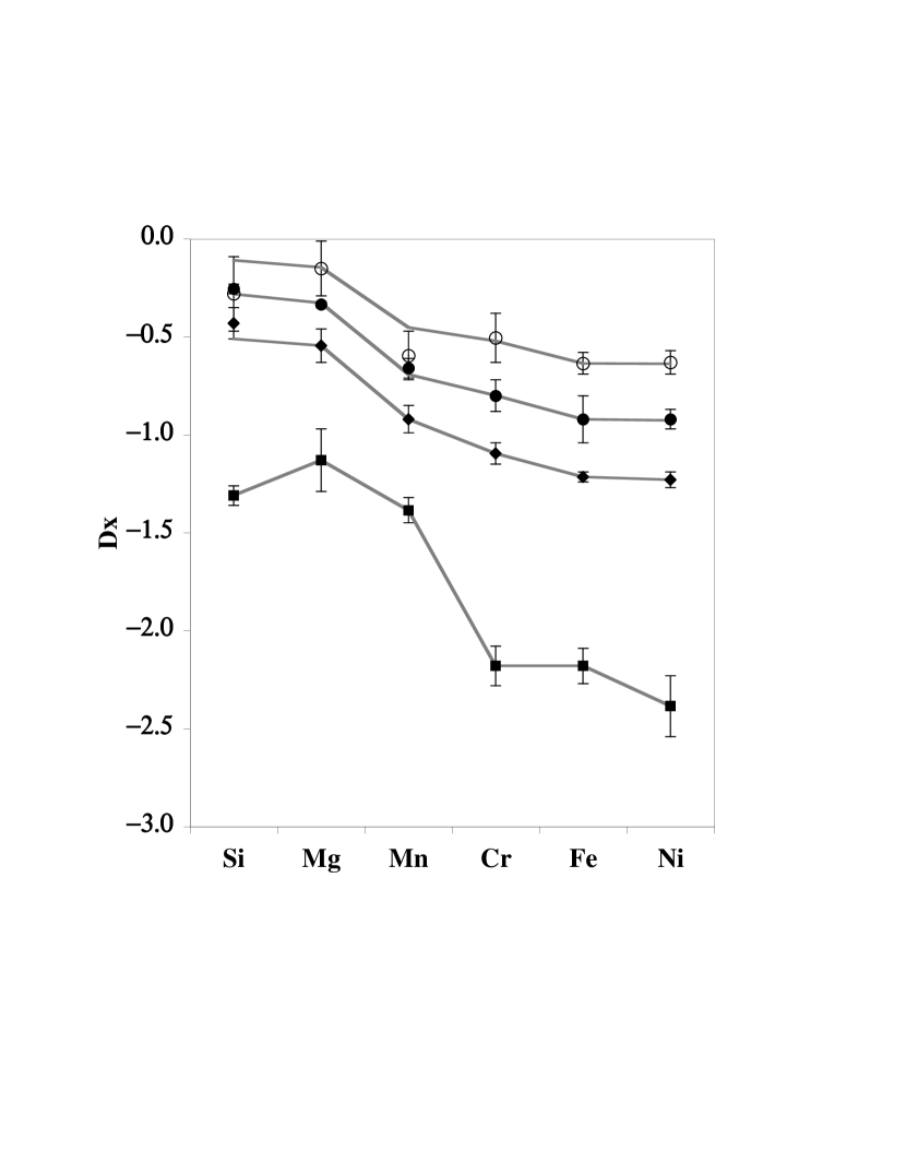
Figure 1: Comparison of observed and predicted interstellar depletion patterns in the Galaxy. Symbols: Galactic patterns observed in the cool disk (squares), the warm disk (diamonds), the warm disk plus halo (filled circles), and the warm halo (empty circles), from Table 6 in SS96. Lines: model predictions obtained from the scaling law (15), derived using the warm disk as the reference depletion pattern and normalized to fit the observed Fe depletions using the values $r_{1}/r_{2}=1.058$, $r_{3}/r_{2}=0.935$, and $r_{4}/r_{2}=0.840$; the parameters $\eta_{\mathrm{x}}$ are taken from Table 1 ($\eta_{\mathrm{x,21}}$).

Here we consider the four types of depletion patterns discussed in SS96 (see Fig. 1). In order of decreasing depletion, these patterns are representative of (1) cool clouds in the Galactic disk, (2) warm clouds in the disk, (3) disk plus halo clouds, and (4) warm halo clouds. The lines of sight considered by SS96 also cover a significant range of extinction properties, with strength of the 217.5 nm emission bump as high as E(bump)=0.89 in HD 24912 and as low as E(bump)=0.00 and 0.36 in HD 38666 and HD 116852, respectively (Savage et al. 1985). We compared pairs of the 4 SS96 depletion patterns to estimate $\eta_{\mathrm{x},ij}$. The results are shown in Table 1, where the quoted errors have been estimated propagating the uncertainties of the fractions in dust. For some elements the $\eta_{\mathrm{x}}$ values obtained from different pairs of patterns show a different behavior depending on whether the warm halo is considered or not. The $\eta_{\mathrm{x}}$ values obtained from cool disk, warm disk and warm disk-plus-halo patterns are in agreement for all elements considered. When we compare the warm halo with the cool and warm disk, the derived parameters for Ni, Cr and Mg are still approximately constant. However, Mn and Si show different values, suggesting that for these elements the rate of incorporation into dust, or detachment from dust, is different when we consider the transition to halo gas.

The approximately constant values of the $\eta_{\mathrm{x}}$ parameters obtained for most elements over a wide range of interstellar conditions encourages us to use relation (15) for modeling all the Galactic depletion patterns. In Fig. 1 we show the results obtained using the warm disk as the $i$-th reference pattern. One can see that all the Galactic patterns can be matched using the set of values $\eta_{\mathrm{x,21}}$ listed in Table 1. In spite of the lack of constancy of $\eta_{\mathrm{Si}}$ and $\eta_{\mathrm{Mn}}$ when the warm halo pattern is considered, the model is capable of fitting also the Si and Mn depletions in the warm halo within the observational errors. Therefore, relation (15) provides an empirical way to express all the different types of depletion patterns by varying only one parameter, $r_{j}/r_{i}$. This is a significant improvement with respect to previous work, in which the fractions in dust were assumed to scale linearly with $r_{j}/r_{i}$ (i.e. $\eta_{\mathrm{x}}=0$ for all elements) and in which by no means was it possible to model at the same type different depletion patterns.

The fact that all types of Galactic depletions can be modeled with a single analytical expression suggests a continuity of the dust properties in different types of interstellar clouds, consistent with results of previous work (Joseph et al. 1986; Joseph 1988; Sofia, Cardelli & Savage 1994). The existence of specific patterns of depletions probably reflects the existence of well defined phases of the ISM, each one with characteristic physical parameters which determine the properties of the dust, as proposed by Spitzer (1985). However, in the transition from disk to halo gas important changes in the dust properties must occur to explain the sudden changes of $\eta_{\mathrm{x}}$ values. These changes are quite significant for Si, suggesting a different behavior of this element as far as its ability to be incorporated in (or detached from) dust grains in different types of interstellar environments.

4 Estimate of the $\varepsilon_{\mathrm{x}}$ parameters from extragalactic studies

If the chemical composition of the medium is not constant, it is necessary to know the $\varepsilon_{\mathrm{x}}$ parameters to apply the scaling law (12). Among the possible choices of $\varepsilon_{\mathrm{x}}$, two values have a special meaning: $\varepsilon_{\mathrm{x}}=0$ implies that the dust composition is insensitive to variations of the overall composition; $\varepsilon_{\mathrm{x}}=1$ implies that dust composition scales in proportion to the composition of the medium, a possibility which seems logical a priori. In addition, the possibility that $\varepsilon_{\mathrm{x}}=1$ is attractive as this would imply that Galactic-type depletion patterns can be applied to studies of galaxies with different chemical compositions. In fact, when $\varepsilon_{\mathrm{x}}=1$, Eq. (12) becomes equal to Eq. (15), i.e. the depletion patterns are of Galactic type independent of any change of the chemical composition of the medium.

As in this study we are not treating the complex mechanisms of dust formation and destruction, we leave the possibility open that $\varepsilon_{\mathrm{x}}$ may take different values. We do not consider, however, values $\varepsilon_{\mathrm{x}}<0$. In fact, negative values would imply that an increase of the abundance of the element X in the medium would lead to a decrease of its abundance in the dust.

In order to constrain the parameters $\varepsilon_{\mathrm{x}}$ we must study interstellar depletions in environments with non-solar abundances. These can be found, for instance, in the ISM of external galaxies. To apply the scaling law to external galaxies we assume that any medium $i$ with specified $r=r_{i}$ and $a_{\mathrm{x}}=a_{\mathrm{x},i}$, even if located in two arbitrary galaxies $A$ and $B$, is characterized by a unique dust composition, i.e. $p_{\mathrm{x}}(r_{i},a_{\mathrm{x},i})_{A}=p_{\mathrm{x}}(r_{i},a_{\mathrm{x},i})_{B}$. From this assumption, from (7) and from (12) we derive an expression which relates the depletions of the $j$-th interstellar medium in the external galaxy $E$ to the depletions of the $i$-th medium in our Galaxy:

$$f_{\mathrm{x},j}=\left({r_{j}\over r_{i}}\right)^{(1+\eta_{\mathrm{x}})}\cdot 10^{\left(\varepsilon_{\mathrm{x}}-1\right)\left[{{\rm X}\over{\rm Y}}\right]_{\mathrm{m},E}}\cdot f_{\mathrm{x},i}~{}~{},$$ (16)

where

$$\left[{{\rm X}\over{\rm Y}}\right]_{\mathrm{m},E}\equiv\log\left({{\rm X}\over{\rm Y}}\right)_{\mathrm{m},E}-\log\left({{\rm X}\over{\rm Y}}\right)_{\sun}~{}~{},$$ (17)

$\left({{\rm X}\over{\rm Y}}\right)_{\mathrm{m},E}$ is the abundance in the medium of the external galaxy, and $\left({{\rm X}\over{\rm Y}}\right)_{\sun}$ is the abundance in the medium of our Galaxy, taken to be solar. Eq. (16) is a generalization of Eq. (11) in Vladilo (1998), which can be derived from (16) for $\eta_{\mathrm{x}}=0$ and $\varepsilon_{\mathrm{x}}=0$.

The scaling law (16) can be used to estimate the depletions in galaxies with non-solar abundances using a well-known Galactic depletion pattern as the reference pattern $i$. As discussed in the previous section, Galactic studies indicate that the $\eta_{\mathrm{x}}$ parameters can be considered approximately constant under different types of interstellar conditions, including variations of the physical state and of the strength of the 217.5 nm emission bump. This gives us confidence to use the values derived in our Galaxy for other galaxies as well, even though, in principle, the adoption of Galactic $\eta_{\mathrm{x}}$ values should be considered as an a priori assumption. As far as the $\varepsilon_{\mathrm{x}}$ parameters are concerned, we can probe their behavior from the study of nearby galaxies with non-solar abundances. For an external galaxy $E$, sufficiently close to measure the gas-phase abundances, $(\mathrm{X\over H})_{\mathrm{g},E}$, and to derive a set of reference abundances from stellar studies, $(\mathrm{X\over H})_{\mathrm{m},E}$, the depletions can be estimated from the expression

$$D_{\mathrm{x},E}~{}=~{}\left[\mathrm{X\over H}\right]_{\mathrm{g},E}-\left[\mathrm{X\over H}\right]_{\mathrm{m},E}~{}=~{}\left[\mathrm{X\over H}\right]_{\mathrm{g},E}-\left[\mathrm{Y\over H}\right]_{\mathrm{m},E}-\left[\mathrm{X\over Y}\right]_{\mathrm{m},E}~{}~{},$$ (18)

where the terms in square brackets are defined as in Eq. (17). It should be noted that not only the model depletions (16), but also the measured depletions (18) change according to the abundance ratios $[\mathrm{X\over Y}]_{\mathrm{m},E}$. If we know these ratios from stellar studies we can compare the observed and predicted depletions and so constrain the parameters $\varepsilon_{\mathrm{x}}$, since we adopt $\eta_{\mathrm{x}}$ from Galactic studies. The Magellanic Clouds (MCs) are ideal targets for applying this technique. A first application is presented in the next Section 4.1.

4.1 Constraints from SMC interstellar studies

Only a few lines of sight have been observed at high spectral resolution in the UV to study interstellar depletions in the MCs. We consider in this study the lines of sight to the SMC stars Sk 78, Sk 108, and Sk 155, for which interstellar column densities of several metals have been obtained from HST observations (Welty et al. 1997, 2001; Koenigsberger et al. 2001) and H I column densities from IUE observations (Fitzpatrick 1985).

To derive the observed depletions (18) we used the gas phase abundances $\left[\mathrm{X/H}\right]_{\mathrm{g,SMC}}$ obtained from the total SMC interstellar column densities (Table 1 in Welty et al. 2001). For the intrinsic SMC metallicity we adopted $\left[\mathrm{Fe/H}\right]_{\mathrm{m,SMC}}=-0.6\pm 0.2$ dex from the typical values of SMC stellar abundances (Russell & Dopita 1992; Welty et al. 1997). This range of metallicity is in agreement with the SMC interstellar [Zn/H] measurements in the same lines of sight, taking into account that Zn is modestly depleted in the Galactic ISM (Roth & Blades 1995). To derive the model depletions (16), we used the fractions in dust $f_{\mathrm{x},i}$ of the Galactic warm disk and the exponents $\eta_{\mathrm{x},21}$ that simultaneously fit all the Galactic ISM patterns (Fig. 1 and Table 1). All the model predictions are normalized to match the SMC iron depletions by varying the parameter $r_{j}/r_{i}$.

As far as the intrinsic SMC abundances $\left[\mathrm{X/Fe}\right]_{\mathrm{\mathrm{m},SMC}}$ are concerned, we first considered the case of solar ratios and then a few non-solar abundance patterns discussed below. In all cases we obtain $r_{j}/r_{i}=0.930,0.802$, and $1.020$ for the sight lines to Sk 78, Sk 108, and Sk 155, respectively. These values of $r_{j}/r_{i}$ are in the range typical of Galactic warm halo, warm disk+halo, and cold disk clouds, respectively (compare with the $r_{j}/r_{i}$ values in the caption to Fig. 1), in agreement with the conclusions pointed out by Welty et al. (1997, 2001).

For the case of solar ratios, i.e. $\left[\mathrm{X/Fe}\right]_{\mathrm{\mathrm{m},SMC}}=0$, the results for the sight lines to Sk 78, Sk 108, and Sk 155 are shown in Figs. 2, 3, and 4, respectively. One can see that the predicted depletions do not fit well the observed ones. In particular, the Si and Mg measurements tend to lie above the predictions while the opposite is true for Mn and Ni. These disagreements cannot be attributed to the uncertainty of the metallicity level. In fact, similar results are found adopting $\left[\mathrm{Fe/H}\right]_{\mathrm{m,SMC}}=-0.8$ dex, and $\left[\mathrm{Fe/H}\right]_{\mathrm{m,SMC}}=-0.4$ dex, the two extreme values of SMC metallicity still consistent with stellar data.

The systematic deviations between observed and predicted depletions suggest that the SMC depletion patterns are peculiar and/or that the SMC relative abundances are non solar. Welty et al. (2001) suggested that the SMC dust may be essentially free of Si and Mg, particularly in the line of sight to Sk 155 where they find exceedingly high [Si/Zn] and [Mg/Zn] ratios. These authors made their analysis assuming solar SMC abundance ratios. In the present work we consider, in addition, the possibility that the SMC abundances have modest deviations from solar ratios.

The SMC abundance pattern is rather uncertain. In Table 2 we list average abundance ratios derived from SMC stellar studies, taken from Russell & Dopita (1992), Hill (1997), and Venn (1999). The observational spread is high and the measurements are often consistent with solar values (Welty et al. 1997). However, tentative evidence of departures from solar ratios is present in the data. In fact, small departures are expected at the metallicity of the SMC. For instance, Milky Way stars with metallicities [Fe/H] $\simeq-0.6$ dex do show characteristic non solar ratios that we also list in Table 2 (from Ryan, Norris & Beers 1996; RNB96). An enhancement of the $\alpha$/Fe ratios [Si/Fe] and [Mg/Fe] and an underabundance of the [Mn/Fe] ratio are present in metal-poor Galactic stars. Even if the SMC has probably undergone a chemical evolution different from that of the Milky Way, we still expect to find a hint of similar deviations in the SMC abundance pattern. For instance, if the chemical evolution has proceeded with a lower rate of (or a more episodic) star formation, the deviations of the $\alpha$/Fe ratios are probably less marked, but still present (Matteucci 1991).

Since modest departures from solar ratios are consistent with SMC stellar data and are expected from the comparison with Galactic stars, it is worth examining if such departures can explain the peculiarities of the SMC depletion patterns. To probe this possibility we adopted the SMC abundance pattern A in Table 2 that was chosen (1) to be consistent with the SMC stellar data and (2) to deviate from solar ratios in the same sense of metal-poor Galactic stars, but by a conservatively low amount. The results obtained adopting the abundance pattern A to represent $\left[\mathrm{Fe/Y}\right]_{\mathrm{\mathrm{m},SMC}}$ are shown in Figs. 5, 6, and 7 for the sight lines to Sk 78, Sk 108, and Sk 155, respectively. In each case, three different values of $\varepsilon_{\mathrm{x}}$ were considered, namely $\varepsilon_{\mathrm{x}}=$ 0, 1, and 2. For $\varepsilon_{\mathrm{x}}=1$, the agreement between observed and predicted depletions is better than in the case of intrinsic solar ratios. For instance, the Si depletion is reproduced within the errors for Sk 78 and Sk 108. However discrepancies are still present for other elements, especially in the sight-line to Sk 155. For $\varepsilon_{\mathrm{x}}$ somewhat below unity the predictions are in agreement with the observations. In fact, all the three depletion patterns, including the peculiar one towards Sk 155, can be simultaneously fit with $0<\varepsilon_{\mathrm{x}}<1$ for most elements considered. For $\varepsilon_{\mathrm{x}}=2$, the discrepancies are even larger than in the case of solar ratios.

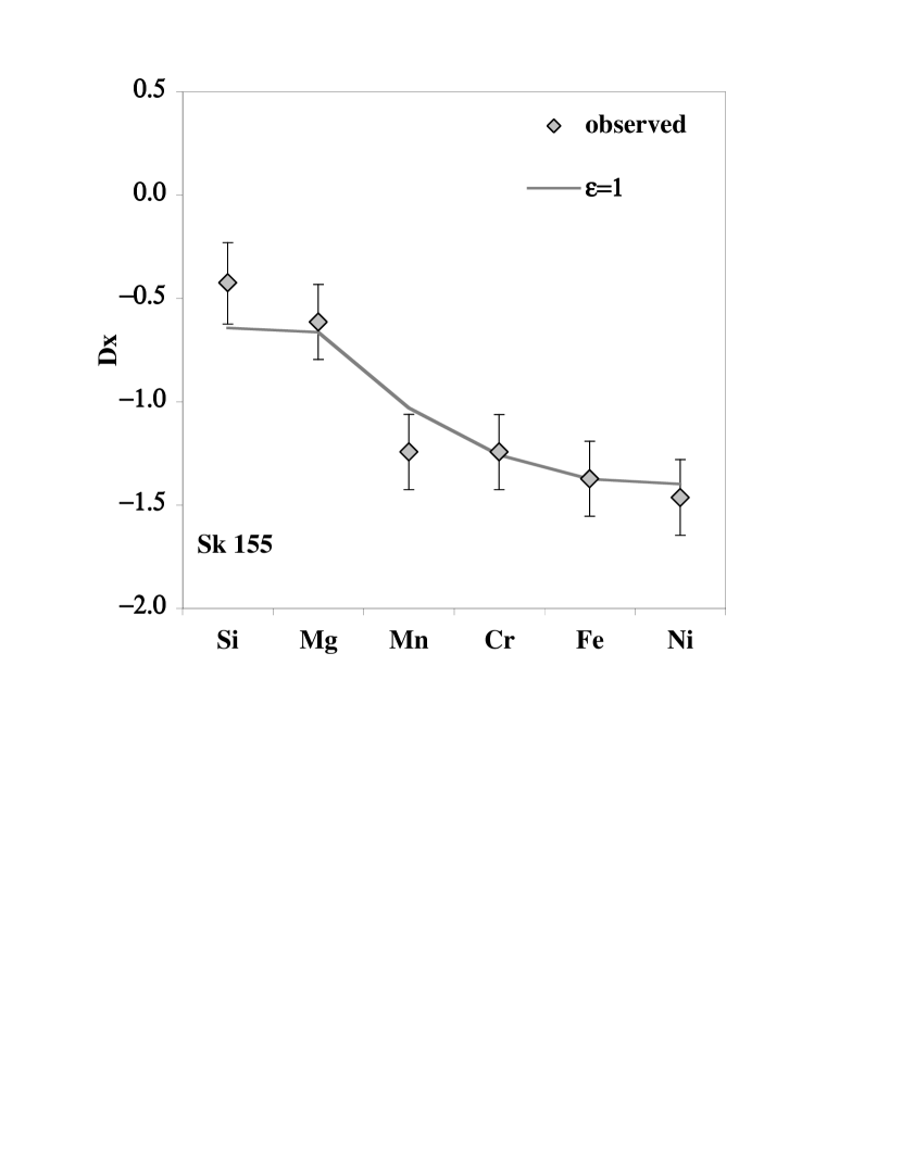
Figure 10: Observed and predicted SMC depletions toward Sk 155. Same as in Fig. 4, but with non solar $\left[\mathrm{X/Fe}\right]_{\mathrm{ref,SMC}}$ ratios (abundance pattern ”B” in Table 2). Thick line: depletions predicted for $\varepsilon_{\mathrm{x}}=1$.

The depletions predicted for $\varepsilon_{\mathrm{x}}\neq 1$ tend to jump to values much lower or higher than the observed depletions. In some cases $\varepsilon_{\mathrm{x}}\neq 1$ all the atoms of an element are predicted to be in dust (Figs. 5 and 7). The curves obtained for $\varepsilon_{\mathrm{x}}=1$ do not suffer from this inconvenience. In addition, the case $\varepsilon_{\mathrm{x}}=1$ is attractive for the reasons explained above (Section 4, first paragraph). We therefore searched for a set of SMC relative abundances able to reproduce the observed depletions while keeping $\varepsilon_{\mathrm{x}}=1$ fixed for all elements. By trial and error we find that the abundance pattern B in Table 2 fits all elements reasonably well. The results for the sightlines to Sk 78, Sk 108, and Sk 155 are shown in Figs. 8, 9, and 10, respectively. It is encouraging that a single set of abundances is able to simultaneously fit the depletions observed in all the three lines of sight with Galactic type depletion patterns (i.e. with $\varepsilon_{\mathrm{x}}=1$). However, at the present time, some of the ratios of the abundance pattern B seem difficult to reconcile with SMC stellar data.

In conclusion, it is not possible to model the SMC depletions if the SMC abundances are strictly solar. We have two choices in modeling the observed depletions: (1) modest departures from solar values (pattern A in Table 2) and $0<\varepsilon_{\mathrm{x}}\leq 1$; (2) ”Galactic type” depletions for all elements ($\varepsilon_{\mathrm{x}}=1$), but larger departures from solar ratios (pattern B in Table 2). Values of $\varepsilon_{\mathrm{x}}$ in excess of unity give depletion patterns inconsistent with the observations.

5 Summary and conclusions

An analytical expression has been derived that allows dust depletions to be estimated in interstellar environments characterized by a wide range of chemical and physical properties. In practice, the depletions are estimated as a function of the dust-to-metals ratio, $r$, and of the relative abundance of the element X in the medium, $a_{\mathrm{x}}$, by scaling a depletion pattern chosen as a reference. The scaling law, given in Eq. (12), has been derived making no assumption on the mechanisms of dust formation, accretion or destruction. No hypothesis has been made on the extinction properties of the dust. The functional form (12) is always valid for infinitesimal changes $\delta r$ and $\delta a_{\mathrm{x}}$. For finite changes $\Delta r$ and $\Delta a_{\mathrm{x}}$ the expression is valid if the parameters $\eta_{\mathrm{x}}$ and $\varepsilon_{\mathrm{x}}$ are constant. These parameters are essentially derivatives of the relative abundance of the element X in the dust, $p_{\mathrm{x}}$. In practice, the parameters $\eta_{\mathrm{x}}$ indicate how the chemical composition of the dust is affected by changes of the dust-to-metals ratio $r$. The parameters $\varepsilon_{\mathrm{x}}$ indicate how the composition of the dust is affected by changes in the composition of the medium.

The scaling law can be applied to interstellar clouds of our Galaxy and of external galaxies with solar or non-solar abundances — including Damped Ly $\alpha$ systems — once the sets of parameters $\eta_{\mathrm{x}}$ and $\varepsilon_{\mathrm{x}}$ are determined. The assumption required to apply the scaling law to external galaxies is that the dust chemical composition is a function of $r$ and $a_{\mathrm{x}}$ valid in any type of interstellar medium. This assumption is much more realistic than assumptions previously adopted in studies of DLA systems, in which depletion patterns were estimated using specific types of Galactic dust.

The parameters $\eta_{\mathrm{x}}$ and $\varepsilon_{\mathrm{x}}$ can be determined empirically by comparing observed depletion patterns in interstellar media with different physical and chemical properties. We have used the typical Milky Way depletion patterns to estimate the parameters $\eta_{\mathrm{x}}$ in environments with variable $r$ but constant (solar) abundances. The resulting values of $\eta_{\mathrm{x}}$ are approximately constant for most elements in a wide range of physical conditions, supporting the validity of the scaling law (12), at least as far as the dependence on $r$ is concerned. With the derived set of $\eta_{\mathrm{x}}$ parameters, the scaling law is able to simultaneously fit all the typical Milky Way depletion patterns by only varying $r$.

The parameters $\varepsilon_{\mathrm{x}}$ can be determined empirically by studying interstellar depletions of galaxies with known abundances different from the solar ones. We have applied this technique to the SMC, for which the intrinsic abundances are constrained from stellar studies and depletion data are available for three lines of sight. The observed SMC depletions can be modeled with the scaling law if the SMC abundance ratios are slightly non solar. The required departures from solar ratios are consistent with the results of SMC stellar studies and with expectations based on Galactic stellar abundances of stars having the same metallicity of the SMC. The agreement between observed and predicted depletions is obtained at values $\varepsilon_{\mathrm{x}}\simeq 1$ or somewhat below unity. With this choice of parameters the scaling law is able to simultaneously fit the three available SMC depletion patterns, including the anomalous pattern observed toward Sk 155. Values $\varepsilon_{\mathrm{x}}>1$ are excluded by the present analysis. The uncertainty of the SMC stellar abundances prevent firmer conclusions or more constrained $\varepsilon_{\mathrm{x}}$ values.

The capability of the scaling relation presented here to match Galactic and SMC depletion patterns is rather encouraging. To probe the general validity of the scaling law it is desirable to measure depletions in a larger number of extragalactic lines of sight. However, these studies will yield stringent constraints only if the intrinsic abundances of the external galaxies, mostly based on stellar observations, will be determined with accuracy. A major step in this direction can be made in the next few years by observing a relatively large number of stars of the Magellanic Clouds at high spectral resolution. These time-consuming efforts will be rewarded by the possibility of modeling interstellar depletions and deriving dust-corrected abundances in high redshift galaxies observed as QSO absorption systems. An implementation of the scaling relation for deriving dust-corrected abundances in Damped Ly $\alpha$ systems will be presented in a separate paper.

Table 1: Empirical determination of the $\eta_{\mathrm{x}}$ parameters

X	$\eta_{\mathrm{x,21}}$	$\eta_{\mathrm{x,31}}$	$\eta_{\mathrm{x,32}}$	$\eta_{\mathrm{x,42}}$	$\eta_{\mathrm{x,41}}$
Si	$+4.68\pm 1.77$	$+5.27\pm 0.60$	$+5.78\pm 1.89$	$+0.87\pm 2.53$	$+1.70\pm 1.94$
Mg	$+3.60\pm 1.50$	$+3.48\pm 0.35$	$+3.37\pm 1.29$	$+3.46\pm 3.98$	$+3.49\pm 3.10$
Mn	$+0.53\pm 0.41$	$+0.69\pm 0.27$	$+0.82\pm 0.60$	$-0.18\pm 0.51$	$-0.02\pm 0.39$
Cr	$+0.37\pm 0.20$	$+0.37\pm 0.29$	$+0.36\pm 0.56$	$+0.45\pm 0.66$	$+0.43\pm 0.52$
Fe	$+0.00\pm 0.07$	$+0.00\pm 0.32$	$+0.00\pm 0.59$	$+0.00\pm 0.19$	$+0.00\pm 0.15$
Ni	$+0.01\pm 0.11$	$+0.02\pm 0.13$	$+0.03\pm 0.26$	$+0.03\pm 0.21$	$+0.02\pm 0.17$

Table 2: Abundance ratios in metal-poor Galatic stars and in the SMC

	RNB96	RD92	H97	V99	A	B
$\left[\mathrm{Si/Fe}\right]$	+0.19	+0.15 $\pm$ 0.22	$-0.14\pm 0.19$	$+0.26\pm 0.19$	+0.10	+0.15
$\left[\mathrm{Mg/Fe}\right]$	+0.12	+0.07 $\pm$ 0.18	$+0.16\pm 0.22$	$-0.01\pm 0.12$	+0.10	+0.10
$\left[\mathrm{Mn/Fe}\right]$	$-$0.30	+0.17 $\pm$ 0.34	$\cdots$	$\cdots$	$-0.10$	$-0.25$
$\left[\mathrm{Cr/Fe}\right]$	$-$0.02	+0.09 $\pm$ 0.24	$-0.31\pm 0.18$	$-0.02\pm 0.13$	+0.00	+0.00
$\left[\mathrm{Ni/Fe}\right]$	+0.00	+0.27 $\pm$ 0.24	$-0.38\pm 0.14$	$\cdots$	+0.00	$-0.10$

Note. — Solar ratios taken from the meteoritic values by Anders & Grevesse (1989). The errors have been computed propagating the errors of each of the two elements considered in the ratio.

Figure 2: Observed and predicted SMC depletion patterns in the line of sight to Sk 78 derived from Eqs. (18) and (16), respectively, for the case of solar $\left[\mathrm{X/Fe}\right]_{\mathrm{ref,SMC}}$ ratios. Symbols: observed depletions obtained using the SMC column densities by Welty et al. (2001), $\log N$(H I)_SMC = $20.93\pm 0.05$ (Fitzpatrick 1985), and $\left[\mathrm{Y/H}\right]_{\mathrm{ref,SMC}}=-0.6$ dex. Line: predicted depletions obtained using the Galactic warm disk as the reference pattern, $r_{j}/r_{i}=0.930$, and the parameters $\eta_{\mathrm{x,21}}$ (see Table 1 and Fig. 1).

Figure 3: Observed and predicted SMC depletion patterns in the line of sight to Sk 108 derived from Eqs. (18) and (16), respectively, for the case of solar $\left[\mathrm{X/Fe}\right]_{\mathrm{ref,SMC}}$ ratios. Symbols: observed depletions obtained using the SMC column densities by Welty et al. (2001), $\log N$(H I)_SMC = $20.54^{+0.11}_{-0.14}$ (Fitzpatrick 1985), and $\left[\mathrm{Y/H}\right]_{\mathrm{ref,SMC}}=-0.6$ dex Line: predicted depletions obtained using the Galactic warm disk as the reference pattern, $r_{j}/r_{i}=0.802$, and the parameters $\eta_{\mathrm{x,21}}$ (see Table 1 and Fig. 1).

Figure 4: Observed and predicted SMC depletion patterns in the line of sight to Sk 155 derived from Eqs. (18) and (16), respectively, for the case of solar $\left[\mathrm{X/Fe}\right]_{\mathrm{ref,SMC}}$ ratios. Symbols: observed depletions obtained using the SMC column densities by Welty et al. (2001), $\log N$(H I)_SMC = $21.54\pm 0.18$ (Fitzpatrick 1985), and $\left[\mathrm{Y/H}\right]_{\mathrm{ref,SMC}}=-0.6$ dex. Line: predicted depletions obtained using the Galactic warm disk as the reference pattern, $r_{j}/r_{i}=1.020$, and the parameters $\eta_{\mathrm{x,21}}$ (see Table 1 and Fig. 1).

Figure 5: Observed and predicted SMC depletions toward Sk 78. Same as in Fig. 2, but with non solar $\left[\mathrm{X/Fe}\right]_{\mathrm{ref,SMC}}$ ratios (abundance pattern ”A” in Table 2). Lines: depletions predicted for different values of $\varepsilon_{\mathrm{x}}$. Dashed line: $\varepsilon_{\mathrm{x}}=0$. Thick line: $\varepsilon_{\mathrm{x}}=1$. Dotted line: $\varepsilon_{\mathrm{x}}=2$. For $\varepsilon_{\mathrm{Mn}}=0$ all the atoms of Mn are predicted to be in dust; a conventional value $D_{\mathrm{Mn,SMC}}=-2$ dex is plotted in the figure.

Figure 6: Observed and predicted SMC depletions toward Sk 108. Same as in Fig. 3, but with non solar $\left[\mathrm{X/Fe}\right]_{\mathrm{ref,SMC}}$ ratios (abundance pattern ”A” in Table 2). Lines: depletions predicted for different values of $\varepsilon_{\mathrm{x}}$. Dashed line: $\varepsilon_{\mathrm{x}}=0$. Thick line: $\varepsilon_{\mathrm{x}}=1$. Dotted line: $\varepsilon_{\mathrm{x}}=2$.

Figure 7: Observed and predicted SMC depletions toward Sk 155. Same as in Fig. 4, but with non solar $\left[\mathrm{X/Fe}\right]_{\mathrm{ref,SMC}}$ ratios (abundance pattern ”A” in Table 2). Lines: depletions predicted for different values of $\varepsilon_{\mathrm{x}}$. Dashed line: $\varepsilon_{\mathrm{x}}=0$. Thick line: $\varepsilon_{\mathrm{x}}=1$. Dotted line: $\varepsilon_{\mathrm{x}}=2$. For $\varepsilon_{\mathrm{Mn}}=0$ and $\varepsilon_{\mathrm{Mg}}=2$ all the atoms of Mn and Mg are predicted to be in dust; conventional values $D_{\mathrm{Mn,SMC}}=D_{\mathrm{Mg,SMC}}=-2$ dex are plotted in the figure.

Figure 8: Observed and predicted SMC depletions toward Sk 78. Same as in Fig. 2, but with non solar $\left[\mathrm{X/Fe}\right]_{\mathrm{ref,SMC}}$ ratios (abundance pattern ”B” in Table 2). Thick line: depletions predicted for $\varepsilon_{\mathrm{x}}=1$.

Figure 9: Observed and predicted SMC depletions toward Sk 108. Same as in Fig. 3, but with non solar $\left[\mathrm{X/Fe}\right]_{\mathrm{ref,SMC}}$ ratios (abundance pattern ”B” in Table 2). Thick line: depletions predicted for $\varepsilon_{\mathrm{x}}=1$.

References

- (1) Anders, E., & Grevesse, N. 1989, Geochim. Cosmochim. Acta, 53, 197
- (2) Centuriòn, M., Bonifacio, P., Molaro, P., & Vladilo, G. 2000, ApJ, 536, 540
- (3) Fedchak, J.A., & Lawler, J.E. 1999, ApJ, 523, 734
- (4) Fitzpatrick, E.L. 1985, ApJS, 59, 77
- (5) Hill, V. 1997, A&A, 324, 435
- (6) Hou, J.L., Boissier, S., Prantzos, N. 2001, A&A, 370, 23
- (7) Howk, J.C., & Savage, B.D., & Fabian, D. 1999, ApJ, 525, 253
- (8) Jenkins, E.B., Savage, B.D., & Spitzer L., Jr. 1986, ApJ, 301, 355 (JSS86)
- (9) Joseph, C.L., 1988, ApJ, 335, 157
- (10) Joseph, C.L., Snow, T.P., Seab, C.G., & Crutcher, R.M. 1986, ApJ, 309, 771
- (11) Koenigsberger, G., Georgiev, L., Peimbert, M., Walborn, N.R., Barbá, R., Niemela, V.S., Morrell, N., Tsvetanov, Z., Schulte-Ladbeck, R. 2001, AJ, 121, 267
- (12) Kulkarni, V.P., Fall, S.M., & Truran, J.W. 1997, ApJ, 484, L7
- (13) Lauroesch, J.T., Truran, J.W., Welty, D.E., & York, D.G. 1996, PASP, 108, 641
- (14) Lu, L., Sargent, W.L.W., & Barlow, T.A. 1996, ApJS, 107, 475
- (15) Matteucci, F. 1991, in SN1987A and other Supernovae, eds. I.J. Danziger & K.Kjar, ESO Proc. 37, (Garching: ESO), 703
- (16) Molaro, P., Bonifacio, P., Centurión, M., D’Odorico, S., Vladilo, G., Santin, P., Di Marcantonio, P. 2000, ApJ, 541, 54
- (17) Morton, D.C. 1974, ApJ, 193, L35
- (18) Pettini, M., Ellison, S.L., Steidel, C.C., Shapley, A.E., & Bowen, D.V. 2000, ApJ, 532, 65
- (19) Pettini, M., King, D.L., Smith, L.J., & Hunstead, R.W. 1997, ApJ, 478, 536
- (20) Pettini, M., Smith, L.J., Hunstead, R.W. & King, D.L. 1994, ApJ, 426, 79
- (21) Prochaska, J.X., & Wolfe, A.M. 1999, ApJS, 121, 369
- (22) Prochaska, J.X., & Wolfe, A.M. 2002, ApJ, in press, (astro-ph/0110351)
- (23) Roth, K.C., & Blades, C., 1995, ApJ, 445, L95
- (24) Russell, S.C., & Dopita, M.A. 1992, ApJ, 384, 508
- (25) Ryan , S.G., Norris, J.E., & Beers, T.C. 1996, ApJ, 471, 254
- (26) Savage, B.D., Massa, D., Meade, M., Wesselius, P.R. 1985, ApJS, 59, 397
- (27) Savage, B.D., & Sembach, K.R. 1996, ARA&A, 34, 279 (SS96)
- (28) Savaglio, S., Panagia, N., & Stiavelli, M. 2000, ASP Conf. Ser. 215, 65
- (29) Sofia, U.J., Cardelli, J.A., & Savage, B.D. 1994, ApJ, 430, 650
- (30) Sofia, U.J., & Meyer, D.M. 2001, ApJ, 554, L221
- (31) Spitzer, L. 1978, Physical Processes in the Interstellar Medium, (New York: Wiley Interscience)
- (32) Spitzer, L. 1985, ApJ, 290, L21
- (33) Tielens, A.G.G.M., Allamandola, L.J. 1987, in Interstellar Processes, ed. D.J. Hollenbach & H.A. Thronson, (Dordrecht: Reidel), 533
- (34) Venn, K.A. 1999, ApJ, 518, 405
- (35) Vladilo, G. 1998, ApJ, 493, 583
- (36) Vladilo, G., Bonifacio, P., Centurión, M., & Molaro, P. 2000, ApJ, 543, 24
- (37) Welty, D.E., Hobbs, L.M., Lauresch, J.T., Morton, D.C., Spitzer, L., & York, D. 1999, ApJS, 124, 465
- (38) Welty, D.E., Lauroesch, J.T., Blades J.C., Hobbs, L.M., & York, D.G. 1997, ApJ, 489, 672
- (39) Welty, D.E., Lauroesch, J.T., Blades J.C., Hobbs, L.M., & York, D.G. 2001, ApJ, 554, L75