Cosmological constraints on quintessential halos

Abstract

A complex scalar field has recently been suggested to bind galaxies and flatten the rotation curves of spirals. Its cosmological behavior is thoroughly investigated here. Such a field is shown to be a potential candidate for the cosmological dark matter that fills up a fraction $\Omega_{\rm\,cdm}\sim 0.3$ of the Universe. However, problems arise when the limits from galactic dynamics and some cosmological constraints are taken simultaneously into account. A free complex field, associated to a very small mass $m\sim 10^{-23}$ eV, has a correct cosmological behavior in the early Universe, but behaves today mostly as a real axion, with a problematic value of its conserved quantum number. On the other hand, an interacting field with quartic coupling $\lambda\sim 0.1$ has a more realistic mass $m\sim 1$ eV and carries a quantum number close to the photon number density. Unlike a free field, it would be spinning today in the complex plane – like the so-called “spintessence”. Unfortunately, the cosmological evolution of such field in the early Universe is hardly compatible with constraints from nucleosynthesis and structure formation.

6 February 2001

I Introduction

The observations of the Cosmic Microwave Background (CMB) anisotropies [1], combined either with the determination of the relation between the distance of luminosity and the redshift of supernovae SNeIa [2], or with the large scale structure (LSS) information from galaxy and cluster surveys [3], give independent evidence for a dark matter density in the range $\Omega_{\rm\,cdm}\,h^{2}=0.13\pm 0.05$ [1], to be compared to a baryon density of $\Omega_{\rm b}\,h^{2}=0.019\pm 0.002$ as indicated by nucleosynthesis [4] and the relative heights of the first acoustic peaks in the CMB data. The nature of that component is still unresolved insofar. The favorite candidate for the non–baryonic dark matter is a weakly–interacting massive particle (WIMP). The so–called neutralino naturally arises in the framework of supersymmetric theories. Depending on the numerous parameters of the model, its relic abundance $\Omega_{\rm\,cdm}$ falls in the ballpark of the measured value. New experimental techniques have been developed in the past decade to detect these evading species. However, detailed numerical simulations have recently pointed to a few problems related to the extreme weakness with which that form of matter interacts. Neutralinos tend naturally to collapse in numerous and highly packed clumps [5] that are not seen – see however [6]. The halo of the Milky Way should contain $\sim$ half a thousand satellites with mass in excess of $10^{8}$ $M_{\odot}$ while a dozen only of dwarf–spheroidals are seen. The clumps would also heat and eventually shred the galactic ridge. More generally, this process would lead to the destruction of the disks of spirals. A neutralino cusp would form at their centers. This is not supported by the rotation curves of low–surface–brightness galaxies that indicate on the contrary the presence of a core with constant density. Finally, two–body interactions with halo neutralinos and its associated dynamical friction would rapidly slow down the otherwise observed spinning bars at the center of spirals like M31.

New candidates for the astronomical dark matter are therefore under scrutiny such as warm dark matter [7], particles with self interactions [8], or non–thermally produced WIMPs [9]. An exciting possibility would be to have a common explanation for both the dark energy $\Omega_{\Lambda}$ and the dark matter $\Omega_{\rm\,cdm}$ components of the Universe. Before trying to reach such an ambitious goal, one could explore the relevance of scalar fields to the cosmological and galactic dark matter puzzles, as was done for dark energy with the so-called “quintessence” models [11]. The archetypal example of quintessence is a neutral scalar field $\varphi$ with Lagrangian density

$${\cal L}\;=\;\frac{1}{2}\,g^{\,\mu\nu}\,\partial_{\mu}\varphi\,\partial_{\nu}\varphi\,-\,V\left(\varphi\right)\;\;.$$ (1)

Should the field be homogeneous, its cosmological energy density would be expressed as

$$\rho_{\varphi}\equiv T^{0}_{\;0}\;=\;{\displaystyle\frac{\dot{\varphi}^{2}}{2}}\,+\,V\left(\varphi\right)\;\;,$$ (2)

whereas the pressure would obtain from $T_{ij}\equiv-g_{\,ij}\,P$ so that

$$P_{\varphi}\;=\;{\displaystyle\frac{\dot{\varphi}^{2}}{2}}\,-\,V\left(\varphi\right)\;\;.$$ (3)

If the kinetic term ${\dot{\varphi}^{2}}/{2}$ is small with respect to the contribution from the potential $V\left(\varphi\right)$, the equation of state can match the condition for driving accelerated expansion in the Universe, $\omega_{Q}\equiv P_{\varphi}/\rho_{\varphi}<-1/3$. Instead, in order to behave as dark matter today, the field should be pressureless: $|P_{\varphi}|\ll\rho_{\varphi}$. So, the kinetic and potential energies should cancel out in Eq. (3), a condition automatically fulfilled by a quickly oscillating scalar field averaged over one period of oscillation. This well–known setup is that of the cosmological axion. It requires a quadratic scalar potential, so that the kinetic and potential energies both redshift as $\varphi^{2}\propto a^{-3}$ with the Universe expansion and cancel out at any time during the field dominated stage, which is then equivalent to the usual matter dominated one.

Axions – or more generally, bosonic dark matter – were revived recently due to the undergoing CDM crisis. For instance, it was noticed in [12] that stucture formation on small scales can be forbidden by quantum mechanics, for wavelengths smaller than the Compton wavelength – i.e., the minimal spreading of an individual boson wave function. The latter matches the scale of galactic substructures for an ultra–light mass of order $m\sim 10^{-22}$ eV. Alternatively, one may introduce a self–coupling term [13, 14]. As we have seen, the existence of a matter–like dominated stage requires that the contribution of non–quadratic terms to the potential energy remains subdominant. Nevertheless, a self–coupling would modify the field behavior in the early Universe, as well as its clustering properties today in regions where the field is overdense – exactly like for boson stars, which are crucially affected by the presence of a self–coupling [15]. The self–coupling is also relevant for the issue of field clumps stability, and can explain why dwarf and low–surface–brightness galaxies have cores with finite density [16].

A remarkable feature with bosonic dark matter is the possibility to form Bose condensates, i.e., large domains where the field is coherent in phase and is in equilibrium inside its own gravitational potential – like boson stars – or in that of an external baryonic matter distribution. This opens the possibility to have a very simple and elegant model for galactic halos, in which rotation curves would follow from simple equations – essentially the Klein–Gordon wave equation, which governs classical scalar fields as well as Bose condensates. This situation strongly differs from the more conventional picture of a gas of individual particles – fermions or heavy bosons – for which gravitational clustering does not lead to universal density profiles and where the shape of galactic halos can only be studied through technically difficult $N$–body simulations.

The formation and stability of such condensates is a complicated issue – see e.g. [19, 20, 21] – even when the field is complex and has a global charge – not to be understood as an electric charge, but as a conserved number of quanta like the baryon or lepton number. For instance, a large condensate can be unstable under fragmentation into smaller clumps. For a real scalar field with no conserved charge, the issue of stability is even more subtle since the field can self–annihilate, especially when the condensate core density exceeds a critical value [19]. This property can improve the agreement with observations [16], since the coupling constant will tune the upper limit on the density of dark matter cusps at the center of galaxies. However, such a positive feature is far from excluding models with a conserved charge. In fact, the issue of Bose condensation on galactic scales – in an expanding Universe – has never been studied in details. The result would depend very much on the scalar potential, and it is difficult to guess what would be the maximal core density today.

In this work, we will focus on the scenario with a conserved charge, and assume that dark matter consists in a complex scalar field with a quasi–homogeneous density in the early Universe, producing later galactic halos through Bose–condensation. The Lagrangian density reads

$${\cal L}\;=\;g^{\mu\nu}\,\partial_{\mu}\phi^{\dagger}\,\partial_{\nu}\phi\;-\;V\left(\phi\right)\,.$$ (4)

Throughout this analysis, we will focus on the potential

$$V\;=\;m^{2}\phi^{\dagger}\phi\,+\,\lambda\,\left\{\phi^{\dagger}\phi\right\}^{2}\;\;.$$ (5)

As a prologue to the study of density perturbations, we will follow the evolution of the homogeneous cosmological background of this field, taking into account the constraints on the scalar potential coming from galactic halos. In a previous work [17], we did a detailed comparison of such halos with universal galactic rotation curves [23], for a massive complex scalar field. We recall the salient features of this analysis in section II and discuss how the corresponding constraint on the mass $m$ is modified when a self–interaction coupling $\lambda$ is introduced. In the subsequent section III, we study how this scenario can be implemented cosmologically. Neglecting the spatial variations of $\phi$, we are led to the cosmological density

$$\rho_{\phi}\;=\;\dot{\phi}^{\dagger}\dot{\phi}\,+\,V\left(\phi\right)$$ (6)

and pressure

$$P_{\phi}\;=\;\dot{\phi}^{\dagger}\dot{\phi}\,-\,V\left(\phi\right)\;\;.$$ (7)

Beside the issue of charge conservation, the case for a complex scalar field is somewhat richer than that of a real (neutral) scalar field. In one limit, the complex field can behave as an effective real one, similar to the usual axion. On the other hand, it can be spinning in the complex plane with slowly–varying modulus, like in the so–called spintessence [18] scenario. This depends on the dominant term in the kinetic energy, which can be either radial and oscillating, or orthoradial and slowly varying. As a result, during the field dominated era, the spintessence would have a continuously vanishing pressure, while the axion pressure would oscillate between $+\rho_{\phi}$ and $-\rho_{\phi}$. Finally, in section IV, we discuss our results and feature the problems that plague the axion–spintessence dark matter scenario. We will suggest some future directions worth being investigated.

II Galactic halos

We are interested in galactic halos consisting in self–gravitating scalar field configurations – which can be seen as Bose–Einstein condensates spanning over very large scales. Since the typical velocities observed in galaxies do not exceed a few hundreds of km.s^-1, it is enough to study the quasi–Newtonian limit where the deviations from the Minkowski metric $\eta_{\mu\nu}={\rm diag}(1,-1,-1,-1)$ are accounted for by the vanishingly small perturbation $h_{\mu\nu}$. Inside galaxies, the latter is of order the gravitational potential

$$h_{\mu\nu}\sim\Phi\sim V_{C}^{2}\;\;,$$ (8)

where $V_{C}$ is the rotation velocity – in the case of spirals – and where $\sqrt{2}\,V_{C}$ is the escape velocity from the system. In the harmonic coordinate gauge where it satisfies the condition

$$\partial_{\alpha}h^{\alpha}_{\;\mu}\,-\,\frac{1}{2}\partial_{\mu}h^{\alpha}_{\;\alpha}\;=\;0\;\;,$$ (9)

the perturbation $h_{\mu\nu}$ is related to the source tensor

$$S_{\mu\nu}\;=\;T_{\mu\nu}\,-\,\frac{1}{2}\,g_{\mu\nu}\,T^{\alpha}_{\;\alpha}$$ (10)

through

$$\Box h_{\mu\nu}\;=\;-\,16\pi\,{\cal G}\;S_{\mu\nu}\;\;.$$ (11)

The Poisson equation reads like

$$\Delta\Phi\;=\;8\pi\,{\cal G}\;S_{00}\;\;,$$ (12)

where $\Phi=h_{00}/2$ is the Newtonian potential. For pressureless matter, $2~{}S_{00}=T_{00}=\rho$. On the other hand, for the complex scalar field, the gravitational potential is sourced by the effective mass density

$${\displaystyle\frac{\rho^{\rm eff}_{\phi}}{2}}\equiv S_{00}\;=\;\left\{2\,\dot{\phi}^{\dagger}\dot{\phi}\,-\,V\left(\phi\right)\right\}$$ (13)

which is a priori different from its cosmological counterpart (6). So, inside a galactic halo, the gravitational potential is given by

$$\Delta\Phi\;=\;4\pi\,{\cal G}\,\left(\rho^{\rm eff}_{\phi}\,+\,\rho_{\rm b}\right)\;\;,$$ (14)

where $\rho_{\rm b}$ is the distribution of baryonic matter forming the various galactic components – stellar disk, bar, bulge… In first approximation, the galaxy can be seen as spherically symmetric. In that case, one shows [22] that all stable field configurations must be in the form

$$\phi(r,t)\;=\;{\displaystyle\frac{\sigma(r)}{\sqrt{2}}}\,e^{\displaystyle i\,\omega t}$$ (15)

where the amplitude $\sigma$ depends only on the radius $r$. Then, the effective field density reads like

$$\rho^{\rm eff}_{\phi}\;=\;\left\{2\,\omega^{2}\sigma^{2}\,-\,m^{2}\sigma^{2}\,-\,\frac{1}{2}\lambda\;\sigma^{4}\right\}\;\;.$$ (16)

The radial distribution of the field $\sigma(r)$ and the gravitational potential $\Phi(r)$ are given by a system of two coupled equations: the Poisson equation (14) and the Klein–Gordon equation. The latter may be expressed as

$$e^{\displaystyle-2v}\,\left\{\sigma^{\prime\prime}\,+\,\left(u^{\prime}+v^{\prime}+\frac{2}{r}\right)\,\sigma^{\prime}\right\}\;+\;\omega^{2}e^{\displaystyle-2u}\,\sigma\;-\;m^{2}\,\sigma\;-\;\lambda\,\sigma^{3}\;=\;0$$ (17)

in the isotropic metric where

$$d\tau^{2}\;=\;e^{\displaystyle 2u}\,dt^{2}\,-\,e^{\displaystyle 2v}\,\left\{dr^{2}+r^{2}d\theta^{2}+r^{2}\sin^{2}\theta\,d\varphi^{2}\right\}\;\;.$$ (18)

The prime denotes the derivative with respect to the radius $r$. The Newtonian approximation corresponds to

$$u\;\simeq\;-\,v\;\simeq\;\Phi\;\;.$$ (19)

Relation (17) simplifies into

$$\Delta\sigma\;+\;\left(1\,-\,4\Phi\right)\,\omega^{2}\,\sigma\;-\;\left(1\,-\,2\Phi\right)\left(m^{2}\,\sigma\;+\;\lambda\,\sigma^{3}\right)\;=\;0\;\;.$$ (20)

For each value of the parameters ($m$, $\lambda$, $\omega$) and a given baryon distribution, these equations form an eigenvalue problem with discrete solutions, labelled either by the central value $\sigma_{0}>0$ or by the number of nodes $n$ in which $\sigma(r)=0$. The lowest energy state – which is not identically null due to charge conservation – has $n=0$. The self–consistency of the Newtonian limit requires $|\Phi|\ll 1$. Such solutions exist only for

$$0<(m^{2}-\omega^{2})\ll m^{2}\;\;.$$ (21)

A Free field

In [17], we solved these equations for $\lambda=0$. We found that halos consisting in the fundamental configuration of a free scalar field fit perfectly well the universal rotation curves of low–luminosity spiral galaxies [23]. These data has three advantages for our purpose: the robustness of the points and error bars – obtained by averaging over many galaxies –, the good determination of the baryon distribution – solely a stellar disk with exponential luminosity profile – and the low baryon contribution which justifies the approximation of spherical symmetry.

With a quadratic potential, the size of the halo is given by

$$l\;\sim\;\sqrt{\frac{M_{P}}{\sigma_{0}}}\,\frac{\hbar}{m\,c}\;\;,$$ (22)

where we neglected the dependence on the baryon density. If the central field value $\sigma_{0}$ is significantly smaller than the Planck mass, the coherence length of the condensate exceeds the Compton wavelength of an individual particle – $l_{\rm compton}=\hbar/(m\,c)$ – but it is clear that only an ultra–light scalar field can condensate on distances of order 10 kpc. The typical orbiting velocity in such a halo is given by $v/c\sim\sqrt{\sigma_{0}/M_{P}}$. Therefore, requiring $v\sim 100$ km.s^-1 and $l\sim 10$ kpc fixes $\sigma_{0}$ around $10^{-6}~{}M_{P}$ and $m$ around $10^{-23}$ eV, as confirmed by a detailed fitting to the data [17].

Since the distribution of such halos only depends on the free parameters $\sigma_{0}$ and $m$ – where we impose a unique value of $m$ for all galaxies – we believe that their success in reproducing universal rotation curves is a significant argument in favor of this model. On the other hand, the existence of such a low mass, even if not strictly forbidden by fundamental principles, is very unlikely due to unavoidable radiative corrections. This could motivate a systematic investigation of other potentials for the scalar field. The next level of complexity would consist in adding a quartic self–coupling.

B Quartic self–coupling $\lambda$

As is well known for boson stars – which are exactly identical to our halos in the absence of a baryon component – the inclusion of a quartic term drastically modifies the mass $m$ and the extension of the condensate, even when it contributes to a negligeable fraction of the central energy density [15, 24]. This is so because $\lambda\,\sigma^{2}$ can be very small with respect to $m^{2}\simeq\omega^{2}$ and yet comparable to the difference $(m^{2}-\omega^{2})$ that appears in the Klein–Gordon equation. In the limit where $\Lambda\equiv\lambda\,/(4\pi\,{\cal G}\,m^{2})\gg 1$ and in the absence of a baryon population, we can even give an exact analytic solution for the field and for the orbiting velocity of test particles:

$$\sigma(r) = \sigma_{0}\left\{{\displaystyle\frac{\sin\left(m\sqrt{2/\Lambda}\,r\right)}{m\sqrt{2/\Lambda}\,r}}\right\}^{1/2}\;\;,$$ (23)

$${\displaystyle\frac{v(r)}{c}} = r\,\Phi^{\prime}(r)\;=\;2\pi~{}\Lambda~{}{\displaystyle\frac{\sigma_{0}^{2}}{M_{P}^{2}}}\left\{{\displaystyle\frac{\sin\left(m\sqrt{2/\Lambda}\,r\right)}{m\sqrt{2/\Lambda}\,r}}\,-\,\cos\left(m\sqrt{2/\Lambda}\,r\right)\right\}\;\;,$$ (24)

with the requirement that

$$\Lambda^{-1}\ll\frac{\sigma_{0}}{M_{P}}\ll\Lambda^{-1/2}\;\;.$$ (25)

Because ${\sigma_{0}}/{M_{P}}\sim{(v/c)}/{\sqrt{\Lambda}}$, the second inequality follows from the Newtonian self–consistency condition $|\Phi|\sim v^{2}\ll 1$. The first inequality translates into $\Lambda\gg\left(c/v\right)^{2}$. It implies that all the field spatial derivatives can be neglected in Eq. (20) and sets the maximal radius up to which the analytic solution is valid. This maximal radius is at most equal to half a period so that $r\leq\sqrt{\Lambda/2}\,(\pi/m)$. That bound is almost saturated for $\Lambda\rightarrow\infty$. Note that $\omega$ does not appear in the analytic solutions because it is only relevant at larger radii. However, the Newtonian self–consistency condition imposes that $1-\omega^{2}/m^{2}\ll 1$.

The field behavior (23) may be readily recovered by neglecting the spatial derivatives of $\sigma$ in the Klein–Gordon equation (20) so that

$$\sigma^{2}(r)\;\simeq\;{\displaystyle\frac{m^{2}}{\lambda}}\,\left\{{\displaystyle\frac{\Omega^{2}}{B}}\,-\,1\right\}\;\;,$$ (26)

where $B(r)=1\,+\,2\,\Phi(r)$ and $\Omega=\omega/m$. In the Newtonian limit, the pressure (7) reads like

$$P_{\phi}\equiv{\cal L}\;\simeq\;{\displaystyle\frac{m^{4}}{4\,\lambda}}\,\left\{{\displaystyle\frac{\Omega^{2}}{B}}\,-\,1\right\}^{2}\;\;,$$ (27)

whilst the effective mass density (16) of the Bose–condensate is

$$\rho^{\rm eff}_{\phi}\;\simeq\;m^{2}\,\sigma^{2}\;\simeq\;{\displaystyle\frac{m^{4}}{\lambda}}\,\left\{{\displaystyle\frac{\Omega^{2}}{B}}\,-\,1\right\}\;\;.$$ (28)

Both are related through the Lane–Emden polytropic equation of state

$$P_{\phi}\;=\;K\,{\rho^{\rm eff}_{\phi}}^{\displaystyle 1+1/n}\;\;,$$ (29)

with $K=\lambda\,/(4\,m^{4})$ while the polytropic index is $n=1$. For such a value, the gravitating system – in hydrostatic equilibrium – is shown to have a constant core radius $r_{c}=\pi\,a$ where

$$a^{2}\;=\;{\displaystyle\frac{1}{8\,\pi\,{\cal G}}}\;{\displaystyle\frac{\lambda}{m^{4}}}\;\;.$$ (30)

The field and density profiles are functions of the reduced radius $z=r/a$

$${\displaystyle\frac{\rho^{\prime}_{\phi}(r)}{\rho^{\prime}_{\phi}(0)}}\;=\;{\displaystyle\frac{\sigma^{2}(r)}{\sigma_{0}^{2}}}\;=\;{\displaystyle\frac{\sin(z)}{z}}\;\;.$$ (31)

The most striking feature in the large $\Lambda$ limit is as follows: although the quartic term remains subdominant in the energy density – Eq. (25) implies that $\lambda\sigma^{4}\ll m^{2}\sigma^{2}$ – the typical size of the system is very different from the free field case since now it reads like

$$l\sim\lambda^{1/2}\,M_{P}\;\hbar/(m^{2}c)\;\;.$$ (32)

As the central field value does not appear in this expression, different halo sizes would just result from different baryon contributions to the density, which bring corrections to (32). The central field value $\sigma_{0}$ still determines the rotation curve amplitude. In the large $\Lambda$ limit and in the absence of baryons, the maximal rotation speed is given exactly by

$${\displaystyle\frac{v_{\rm max}^{2}}{c^{2}}}\;=\;2.13~{}\pi~{}\Lambda\,{\displaystyle\frac{\sigma_{0}^{2}}{M_{P}^{2}}}\qquad{\rm at}\qquad r\;=\;1.94\,\Lambda^{1/2}\,/\,m\;\;.$$ (33)

In this paper, we will not extend our previous comparison with galactic rotation curves [17] to the case of a quartic self–coupling, leaving this for a future publication. We will just use relations (32) and (33) in order to find a rough order of magnitude estimate for $\lambda/m^{4}$ which has the best chance to provide a good fit to the data. In the next section, this constraint will be plugged into a cosmological dark matter scenario. By requiring that the rotation velocity peaks around 200 km.s^-1 at a typical radius of 10 kpc, we find

$$m\sim\lambda^{1/4}\;{\rm eV}\qquad{\rm and}\qquad\sigma_{0}\sim\Lambda^{-1/2}\;10^{-3}\;M_{P}\;\;.$$ (34)

Taking for instance $\lambda$ in the range $[1\,,\,10^{-4}]$, we obtain a mass of order 0.1 to 1 eV, i.e., a few orders of magnitude larger than the expected neutrino masses. This gives $\Lambda\sim 10^{52}$ and $\sigma_{0}\sim 0.1$ eV.

III Cosmological dark matter

A Matter–like behavior

A homogeneous complex scalar field with a quadratic potential is a perfect candidate for pressureless cold dark matter. Let us write the Klein–Gordon and Friedman equations for the field configuration

$$\phi(t)\;=\;{\displaystyle\frac{\sigma(t)}{\sqrt{2}}}\,e^{\displaystyle i\,\theta(t)}\;\;.$$ (35)

This amounts to

$${\displaystyle\frac{d^{2}\sigma}{dt^{2}}}+\frac{3}{a}{\displaystyle\frac{da}{dt}}{\displaystyle\frac{d\sigma}{dt}}+m^{2}\sigma+\lambda\sigma^{3}-\omega^{2}\sigma = 0\;\;,$$ (36)

$${\displaystyle\frac{d\omega}{dt}}\sigma+\frac{3}{a}{\displaystyle\frac{da}{dt}}\omega\sigma+2\omega{\displaystyle\frac{d\sigma}{dt}} = 0\;\;,$$ (37)

$$3H^{2}=3\left({\displaystyle\frac{da}{a\,dt}}\right)^{2}=8\pi\,{\cal G}\;\left[\,\rho_{\rm rad}^{\mbox{ }}\right. + \left.\frac{1}{2}\left\{\left({\displaystyle\frac{d\sigma}{dt}}\right)^{2}+\omega^{2}\sigma^{2}+m^{2}\sigma^{2}+\frac{\lambda}{2}\sigma^{4}\right\}\right]\;\;$$ (38)

where $\rho_{\rm rad}$ is the usual density of relativistic photons and neutrinos and $\omega=d\theta/dt$. The second equation implies the conservation of the charge per comoving volume $Q=\omega\sigma^{2}a^{3}$. Therefore, we can rewrite the first equation as

$${\displaystyle\frac{d^{2}\sigma}{dt^{2}}}+\frac{3}{a}{\displaystyle\frac{da}{dt}}{\displaystyle\frac{d\sigma}{dt}}+m^{2}\sigma+\lambda\sigma^{3}-{\displaystyle\frac{Q^{2}}{\sigma^{3}a^{6}}}=0\;\;.$$ (39)

It is most convenient to use the dimensionless time and field variables:

$$\tilde{t}=mt~{},\qquad\tilde{H}=H/m,\qquad u=\sqrt{\frac{m}{Q}}a^{3/2}\sigma~{}.$$ (40)

Then, the charge conservation implies $\omega\,u^{2}=m$ and the Klein–Gordon equation reads like

$$\ddot{u}+\left\{1-u^{-4}+\frac{\lambda Q}{a^{3}m^{3}}u^{2}-\frac{3}{2}\left(\dot{\tilde{H}}+\frac{3}{2}\tilde{H}^{2}\right)\right\}u=0\;\;,$$ (41)

where the dot denotes a derivative with respect to $\tilde{t}$. When $\lambda\neq 0$, we see that the self–coupling term always dominates the mass term in the past, when $a\rightarrow 0$. However, we will first study the opposite case when the quartic term is zero or subdominant. If Eq. (41) is to be applied today, or in the late stage of evolution of the Universe, we can also neglect the contribution from the Universe expansion: today, one has $H_{0}\sim 10^{-61}M_{P}$, many orders of magnitude below the values of $m$ discussed in section II. So, Eq. (41) reduces to

$$\ddot{u}+u-u^{-3}=0\;\;,$$ (42)

and describes some periodic oscillations in a static potential $V(u)\equiv(u^{2}+u^{-2})/2$, with a minimum at $u_{0}=1$ corresponding to $\omega=m$. The field density reads

$$\rho_{\phi}=m\,Q\,E_{u}\,a^{-3}\;\;,$$ (43)

where $E_{u}\geq 1$ stands for the conserved energy $(\dot{u}^{2}+u^{2}+u^{-2})/2$. We conclude that in the late evolution of the Universe, as soon as $m$ becomes bigger than $H$ and $\lambda^{1/2}\sigma$, the homogeneous scalar field behaves exactly as a cosmological background of dark matter.

Let us provide further intuition on the physical meaning of the oscillations for the variable $u$. If $E_{u}\simeq 1$ and $u$ is almost stable around one, then the modulus slowly decreases as $\sigma\propto a^{-3/2}$, while the phase velocity is constant with $\omega=m$. The equation of state is that of pressureless matter:

$$w=\frac{P_{\phi}}{\rho_{\phi}}\sim\frac{H^{2}}{m^{2}}\ll 1\;\;.$$ (44)

Such a field, following a spiral trajectory, is a particular case of what was recently called spintessence [18]. On the other hand, when $E_{u}\gg 1$, $u$ and $\omega$ strongly oscillates, but the trajectory of $u\,e^{\displaystyle i\theta(t)}$ is a fixed ellipse as can be seen from the exact analytic solution to Eq. (42):

$$u=\left\{\left(E_{u}^{2}-1\right)^{1/2}\sin\left(2\tilde{t}+\alpha\right)+E_{u}\right\}^{1/2},\qquad\theta\left(\tilde{t}=\pi\right)-\theta(0)=\int_{\displaystyle 0}^{\displaystyle\pi/m}\!\!\!\!\!\omega(t)dt=\int_{\displaystyle 0}^{\displaystyle\pi}u^{-2}\,d\tilde{t}=\pi\;\;.$$ (45)

The integral of the phase over one period of oscillation obtains from Gradshteyn and Ryzhik, 3.661.4. So, the field $\phi$ follows an ellipse which axes decrease as $a^{-3/2}$. In the large $E_{u}$ limit, the ellipse is squeezed and reduces asymptotically to a line. Then, the complex field is essentially similar to a real oscillating field, like in usual axionic dark matter models. The pressure does not vanish identically, but quickly oscillates between $+\rho_{\phi}$ and $-\rho_{\phi}$, with zero average over one period $\Delta t=\pi/m$. This period is much smaller than $H^{-1}$: on cosmological scales, the field still has the same effect as pressureless matter.

B radiation domination: the $\lambda=0$ case

In the $\lambda=0$ case, we know that the mass should be of order $m\sim 10^{-23}$ eV, ten orders of magnitude above the present value of the Hubble parameter. It is easy to show that $H$ will start to dominate over the mass at a redshift of order $6\times 10^{5}$. Therefore, the previous analytic solutions (43) and (45) only apply to the end of the radiation dominated stage. During radiation domination, the Klein–Gordon equation (41) simplifies into

$$\ddot{u}+u+\frac{3}{4}\tilde{H}^{2}u-u^{-3}=0\;\;.$$ (46)

When $H\gg m$ – i.e., $\tilde{H}\gg 1$ – the term $u$ can be neglected in the above equation. We then obtain a simple non–linear equation for the variable $v=a^{-1/2}u$

$$v^{\prime\prime}-\frac{1}{v^{3}}=0\;\;,$$ (47)

where the prime denotes derivation with respect to conformal time $d\tilde{t}=a\,d\tau$. There is an exact solution:

$$\sigma=\sqrt{\frac{Q}{m}}\,\frac{v}{a}=\left\{C_{1}+\frac{C_{2}}{a}+\frac{C_{3}}{a^{2}}\right\}^{1/2}\;\;.$$ (48)

Only two of the three constants ($C_{1}$, $C_{2}$, $C_{3}$) are independent since

$$C_{1}C_{3}=\frac{C_{2}^{2}}{4}+\frac{Q^{2}}{(a^{2}H)^{2}}\;\;.$$ (49)

Remember that $a^{2}H$ is also constant during radiation domination. The free parameters ($C_{1}$, $C_{2}$) can be conveniently expressed as a function of the initial conditions for the field at some initial time $t_{i}$:

$$C_{1} = \sigma_{i}^{2}+\frac{2\sigma_{i}(d\sigma/dt)_{i}}{H_{i}}+\frac{(d\sigma/dt)_{i}^{2}}{H_{i}^{2}}+\frac{\omega_{i}^{2}\sigma_{i}^{2}}{H_{i}^{2}}\;\;,$$ (50)

$$C_{2} = -2a_{i}\left\{\frac{\sigma_{i}(d\sigma/dt)_{i}}{H_{i}}+\frac{(d\sigma/dt)_{i}^{2}}{H_{i}^{2}}+\frac{\omega_{i}^{2}\sigma_{i}^{2}}{H_{i}^{2}}\right\}\;\;.$$ (51)

These results show that $\sigma$ quickly stabilizes at a value $\sqrt{C_{1}}$. During radiation domination, the field energy density reads like:

$$\rho_{\phi}\;=\;{\displaystyle\frac{(a^{2}H)^{2}}{2}}{\displaystyle\frac{C_{3}}{a^{6}}}\,+\,{\displaystyle\frac{m^{2}}{2}}\left\{C_{1}+\frac{C_{2}}{a}+\frac{C_{3}}{a^{2}}\right\}\;\;.$$ (52)

Interestingly, we see that after some time the energy can be dominated by the contribution of the mass term, even if the latter can be neglected in the Klein–Gordon equation.

We now understand what the generic evolution looks like, starting from an early time – say, for instance, at the end of reheating – at which the field density is smaller than the radiation density: first, $\rho_{\phi}$ decays as $a^{-6}$; then, it stabilizes around the value $m^{2}C_{1}/2$, and remains constant as long as $H>m$; finally, when $H<m$, the density decays as that of pressureless matter, takes over the radiation density, and drives the matter–like dominated stage. Such a scenario requires a single constraint: the constant value of the field density during radiation domination should be matched with the matter density extrapolated from today back to the time $t_{*}$ at which $H=m$:

$$\frac{m^{2}}{2}\,C_{1}\;=\;\Omega_{\rm\,cdm}\,\rho_{c}^{0}\,\left(\frac{a_{0}}{a_{*}}\right)^{3}\qquad\Rightarrow\qquad C_{1}\sim 7\times 10^{-4}\,M_{P}^{2}\;\;.$$ (53)

The scenario is enough constrained to reach another conclusion: when the field density decays as matter, its dynamics is that of an effective oscillating real scalar field and not that of spintessence. Indeed, as soon as the density becomes constant during radiation domination, one has

$${\displaystyle\frac{(a^{2}H)^{2}}{2}}\,{\displaystyle\frac{C_{3}}{a^{6}}}\ll{\displaystyle\frac{m^{2}}{2}}\,C_{1}\qquad\Rightarrow\qquad{\displaystyle\frac{Q^{2}}{a^{6}}}\ll m^{2}C_{1}^{2}\;\;.$$ (54)

On the other hand, a crude matching between the two expressions for the energy density (43) and (52) at the time when $H=m$ gives:

$$m\,Q\,E_{u}\,a^{-3}\sim m^{2}\,C_{1}\qquad\Rightarrow\qquad\frac{Q^{2}}{a^{6}}\,E_{u}^{2}\sim m^{2}\,C_{1}^{2}\;\;.$$ (55)

By combining Eq. (54) and (55), we find that $E_{u}^{2}\gg 1$, which is the condition for the field trajectory in the complex plane to be a squeezed ellipse of constant phase.

So far, we have assumed that the radiation density was initially dominant, in order to use the analytic solutions (48) and (52). Instead, if the field dominates initially – a situation that could be allowed before the time of Big Bang Nucleosynthesis (BBN) – the field density will nevertheless decay as $a^{-6}$. Indeed, if $\rho_{\phi}\geq\rho_{\rm rad}$, then necessarily $\rho_{\phi}\gg m^{2}\sigma^{2}$. We conclude that $P_{\phi}=\rho_{\phi}$, and energy conservation implies that $\rho_{\phi}\propto a^{-6}$. As soon as the radiation density takes over, the previously described analytic solutions do apply.

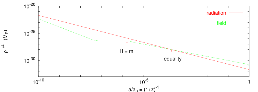
FIG. 1.: Evolution of the field and matter densities, in the scenario with $\lambda=0$ and $m\sim 10^{-23}$ eV. The evolution starts at a redshift $z=10^{10}$ – but we could have equally well started earlier. The initial value of the field density can be chosen arbitrarily, below or above that of radiation density. After decaying as $a^{-6}$, the field density reaches a plateau which amplitude has been fixed according to Eq. (53). This condition ensures a correct value of the density today: $\rho_{\phi}=\Omega_{\rm\,cdm}\rho_{\rm c}^{0}$. At $z=6.3\times 10^{5}$, when $H=m$, the density starts to decrease as $a^{-3}$, like for presureless matter, and takes over radiation at $z\simeq 3\times 10^{3}$.

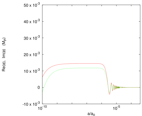
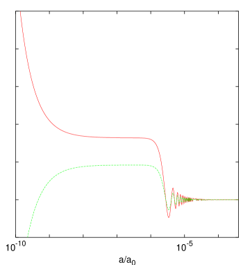
FIG. 2.: Two possible evolutions of the field real and imaginary parts, in the scenario with $\lambda=0$ and $m\sim 10^{-23}$ eV. On the left panel, the initial field modulus has been chosen below the equilibrium value $\sqrt{C_{1}}$ as determined in Eq. (53). The opposite situation is shown on the right panel. In both cases, the field density decays like in Fig. 1. At redshift $z=6.3\times 10^{5}$, when $H=m$, the field starts to oscillate, but its density decays smoothly as that of presureless matter. Because the real and imaginary parts are exactly in phase, the field is equivalent to a single real scalar field.

C radiation domination: $\lambda\neq 0$

If the field has got a quartic self–coupling, $\lambda\sigma^{4}$ must be negligible with respect to $m^{2}\sigma^{2}$ in the late Universe in order to drive a matter–like dominated stage with $\rho_{\phi}\propto a^{-3}$. However, a quartic self–coupling is likely to be cosmologically relevant at early times, whenever the field modulus $\sigma$ well exceeds $\lambda^{-1/2}\,m$. In that case, the equation for $v$ – see relation (47) – reads like

$$v^{\prime\prime}-\frac{a^{\prime\prime}}{a}\,v+\frac{\lambda\,Q}{m^{3}}\,v^{3}-\frac{1}{v^{3}}=0\;\;.$$ (56)

During radiation domination, $a^{\prime\prime}=0$ and $v$ is a periodic – elliptic – function, describing non–harmonic oscillations in the potential $V(v)=\lambda\,Q\,v^{4}/(4\,m^{3})\;+\;1/(2\,v^{2})$, with a minimum at $v_{0}=\left\{m^{3}/(\lambda Q)\right\}^{1/6}$. The period of the oscillations – expressed in conformal time – is of order $m(Q\lambda)^{-1/3}$. So, $\sigma$ performs damped oscillations with a constant period $\Delta a\sim a^{2}H(Q\lambda)^{-1/3}$ with respect to the scale factor. If we furthermore define the conserved pseudo–energy energy of $v$ by $E_{v}=v^{\prime 2}/2+V(v)$, we can express the field density as

$$\rho_{\phi}=m\,Q\,\left\{E_{v}-\frac{Ha}{m}\,v\,v^{\prime}+\frac{H^{2}a^{2}}{2\,m^{2}}v^{2}\right\}a^{-4}\;\;.$$ (57)

Remember that $Ha$ decays as $a^{-1}$ during radiation domination: a priori, at early times, the field density performs damped oscillations like the field modulus while at late times it decays smoothly, as for radiation

$$\rho_{\phi}=m\,Q\,E_{v}a^{-4}\;\;.$$ (58)

The transition between both behaviors takes place when $H^{2}a^{2}v^{2}\sim m^{2}E_{v}$, where $v$ is evaluated at the maximum of one oscillation: $v_{\rm max}\sim(4m^{3}E_{v}/\lambda Q)^{1/4}$. Inserting this condition in Eq. (57), we find that the transition between damped oscillations and smooth decay occurs when $\rho_{\phi}\simeq H^{4}/\lambda$. In practice, this implies that the oscillatory behavior is generally irrelevant unless $\lambda$ is fine–tuned to extremely small values – for the ordinary radiation component, the condition $\rho_{\rm rad}\gg H^{4}$ is already realized at the end of inflation. So, Eq. (58) applies even in the early Universe.

Later on, the transition between radiation–like and matter–like behaviors will be effective when the maximal value of $\sigma$ during one oscillation, computed from Eq.(56), will be comparable to $\lambda^{-1/2}m$. This translates into

$$\sigma_{\rm max}=\sqrt{\frac{Q}{m}}\frac{v_{\rm max}}{a}=\frac{1}{a}\left(\frac{4mQE_{v}}{\lambda}\right)^{1/4}=\frac{m}{\sqrt{\lambda}}\qquad\Rightarrow\qquad a=\left(\frac{4\lambda QE_{v}}{m^{3}}\right)^{1/4}\qquad\Rightarrow\qquad\rho_{\phi}\sim\frac{m^{4}}{\lambda}\simeq({\rm eV})^{4}\;\;.$$ (59)

In the last equality we used the constraint from the size of galactic halos. Since, on the other hand, $\rho_{\rm eq}\sim 0.55\,({\rm eV})^{4}$, the transition to matter–like behavior occurs slightly before equality. This means that at earlier times, when the field behaves like radiation, its density should be fine–tuned in order to be close to the radiation density.

This scenario is illustrated on Fig. 3. In order to obtain the correct value of the field and radiation densities today, $\rho_{\phi}$ must be adjusted to $0.6\,\rho_{\rm rad}$. This would correspond to an effective number of extra neutrino species of $\Delta N_{\rm eff}=5$ that is not even allowed by BBN.

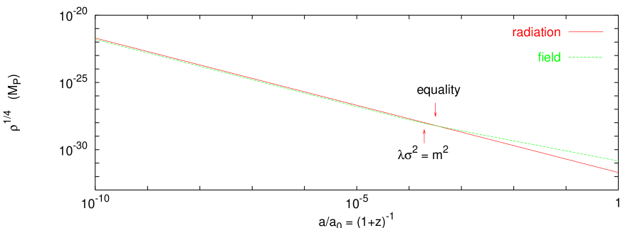
FIG. 3.: Evolution of the field and matter densities, in the scenario with $m\sim\lambda^{1/4}$ eV and arbitrary $\lambda$. The evolution also starts at a redshift $z=10^{10}$. The field decays first as dark radiation, and then as dark matter. The transition between these two regimes is constrained by Eq. (59) to take place immediately before matter–radiation equality. In other words, in the early Universe, the field density must be very close to that of radiation. The simulation gives $\rho_{\phi}=0.6\,\rho_{\rm rad}$ in order to obtain a correct value of $\rho_{\phi}=\rho_{\rm cdm}$ today (such that $\Omega_{\rm cdm}\,h^{2}=0.13$).

IV Discussion

In section II, we recalled why a complex scalar field is an attractive candidate for dark matter in galactic halos; it can provide a rather powerful explanation to the observed rotation curves, because the radial distribution of a scalar field after Bose condensation is constrained by a wave equation (the Klein–Gordon equation); this form of dark matter would be very smooth, and unlike a gas of individual particles, it would not slow down the relative motion of the baryonic components through dynamical friction.

The results of section III show that the complex scalar field can also play the role of a cosmological dark matter background, since after various possible behaviors in the early Universe, which depend on the exact shape of the potential, the field will decay like ordinary pressureless matter as soon as the mass term dominates the potential and the mass is bigger than the Hubble parameter.

However, when the parameters of the scalar potential are estimated from the size and mass of galactic halos, and plugged into the cosmological evolution, some tension appears both for the free–field model and for the one with a quartic self–coupling. Indeed, the redshift at which the field starts to decay like matter, $\rho_{\phi}\propto a^{-3}$, is completely fixed by these parameter values.

In the case with $\lambda=0$, this transition occurs at a redshift close to $z=6\times 10^{5}$. The comoving wavenumber of perturbations entering into the Hubble radius at that time is $k=3$ Mpc^-1. As shown in Ref.[12], this is of the same order of magnitude as the Jeans length for the free field. So, larger wavelengths – in particular, those probed by the spectrum of CMB anisotropies and by the linear matter power spectrum – are expected to undergo the same evolution as in an ordinary CDM model. On smaller wavelength, one would still need to prove with numerical simulations that Bose condensation can occur on the scale of galactic halos – and eventually also on slightly bigger and smaller scales. So far, this model still sounds attractive, apart maybe from the ultra–light mass required ($m\sim 10^{-23}$eV).

In the case with $\lambda\neq 0$, the transition between radiation–like and matter–like behaviors happens even later, just before equality; therefore, the field density during radiation domination has to be very close to that of photons and neutrinos. Our simulation reveals that $\Omega_{\rm cdm}h^{2}=0.13$ today obtains from $\rho_{\phi}/\rho_{\rm rad}\simeq 0.6$ during radiation domination; in other words, the field contributes to the number of relativistic degrees of freedom as an effective neutrino number $\Delta N_{\rm eff}\simeq 5$, in contradiction with the BBN constraint $|\Delta N_{\rm eff}|\leq 1$. Moreover, the perturbations which enter into the Hubble radius before the transition – which would be probed today by the spectrum of CMB anisotropy and the linear matter power spectrum, since their comobile wavenumber is bigger than $k\sim 10^{-2}$ Mpc^-1 – would be suppressed with respect to CDM perturbations (essentially, like for hot dark matter). These problems were previously noticed by Peebles [13] in the case of a real scalar field. As a possible solution, Peebles suggests a polynomial self–coupling with a power slightly smaller than four. In fact, in order to save this scenario, it would be enough to increase the redshift of the transition by a factor ten or so. We conclude that the model with a quartic self–coupling is marginally excluded by cosmological constraints, but that any small deviations from the simple framework studied here are worth being investigated.

Our analysis is still incomplete. We said that the conservation of the charge $J_{0}=i(\phi^{*}\dot{\phi}-\phi\dot{\phi}^{*})$ was crucial for the stability of the condensates. Charge conservation also provides further constraints between, on the one hand, the cosmological background of the field in the early Universe, and on the other hand, the current distribution of dark matter in the form of field condensates. Also, it can give some hints on possible mechanisms for the generation of the field density in the early Universe. In terms of quanta, the conservation of charge implies a constant number of bosons minus anti-bosons inside a comoving volume:

$$Q=(n_{\phi}-n_{\bar{\phi}})a^{3}={\rm cte}\;\;,$$ (60)

where ($n_{\phi}$, $n_{\bar{\phi}}$) are the number density of bosons and of their CP conjugates. We want to evaluate this number today in the form of galactic dark matter. A priori, the rotating phase inside each condensate is fixed up to an arbitrary sign: $\theta(t)\simeq\pm\,m\,t$. So, some halos can be made of bosons, and some others of anti–bosons. This may occur, for instance, if the scalar field was populated during a phase transition: after the transition, the initial field distribution could be very homogeneous, but with an arbitrary phase distribution, leading to domains with positive and negative values of $\omega=d\theta/dt$. A priori, such a disordered initial configuration – with no phase coherence – may not exclude the subsequent formation of Bose condensates. In this case, the mean number density of bosons minus anti–bosons today can be arbitrarily close to zero, and the conservation of charge does not give any new constraint. Note however that two halos of opposite charge could annihilate and radiate out a massive amount of energy. Although this issue would deserve a more careful study, it is probably in conflict with observations.

Let us consider now the case where all galaxies carry a charge with same sign. This can occur if the field underwent inflation – or was coupled to a field that underwent inflation – in such way to be very homogeneous in the early Universe, as assumed in section III. Then, at the beginning of the matter–like regime, the phase would be coherent even on super–horizon scales, and all condensates would form with the same rotating phase. We can estimate the charge in galaxies, $Q_{\rm gal}$, by multiplying the typical charge of a single halo by the number density of halos. This charge must be smaller than or equal to the total charge of the cosmological homogeneous background, $Q_{\rm tot}=\omega\,\sigma^{2}a^{3}$.

In the $\lambda=0$ case, the charge inside one halo is given by [22, 17]:

$$N\sim\sqrt{\frac{\sigma_{0}}{M_{P}}}\,\frac{M_{P}^{2}}{m^{2}}\sim 10^{99}\;.$$ (61)

Under the very crude assumption that the Universe contains in average one halo per volume ${\cal V}=1$ Mpc³, we find a mean density today

$$n_{\phi}=Q_{\rm gal}\;a_{0}^{-3}\sim N/{\cal V}\sim 10^{25}{\rm cm}^{-3}\;.$$ (62)

This number is extremely large, $10^{22}$ times bigger than the present number density of photons. This is a strong indication that the model is not realistic: it would be very difficult to generate such a huge charge in the early Universe. In fact we can even completely exclude the model by comparing $Q_{\rm gal}$ with the total charge of the cosmological background. We saw in section III, Eqs.(54, 55), that the existence of a plateau for $\rho_{\phi}$ during radiation domination imposes today a field dynamics close to that of an oscillating real axion, rather than spintessence. For spintessence, the number density $n_{\phi}=Q_{\rm tot}\,a^{-3}$ is equal to $\rho_{\phi}/m$ as can be seen from Eq.(43) with $E_{u}=1$. For an oscillating axion, most of the kinetic energy is in the radial direction and $n_{\phi}\ll\rho_{\phi}/m$ since the term $E_{u}$ in relation (43) is now much larger than 1. Because we must be in the latter case at least during matter domination, we find the following upper bound on the total charge today:

$$n_{\phi}=Q_{\rm tot}\,a_{0}^{-3}\ll\frac{\Omega_{\rm cdm}\,\rho_{\rm c}^{0}}{m}\simeq 10^{23}{\rm cm}^{-3}\;.$$ (63)

We find $Q_{\rm tot}\ll Q_{\rm gal}$, which is impossible. We conclude that the present dark matter scenario, based on a complex free scalar field forming galactic halos after Bose condensation, is not consistent – at least when the field is assumed to be homogeneous in the early Universe, and today all condensates carry a charge with the same sign. It would certainly be interesting to investigate the opposite scenario, with a homogeneous initial density but random phases, with the drawback that halos and “anti-halos” may annihilate.

As we have seen, the case $\lambda\neq 0$ is already marginally excluded by cosmological constraints, but it is worth calculating the various charges also for this model. An individual halo has got a charge – see relation (34) –

$$|N|\sim\frac{\sigma_{0}^{2}\,\lambda^{3/2}M_{P}^{3}}{m^{5}}\sim\left(\frac{1{\rm eV}}{m}\right)10^{75}\;\;.$$ (64)

Under the assumption that all halos have a positive charge, one finds

$$n_{\phi}=Q_{\rm gal}\,a_{0}^{-3}\sim N/{\cal V}\sim 30\,{\rm cm}^{-3}\;\left(\frac{1{\rm eV}}{m}\right)\;\;.$$ (65)

We are led to two intriguing coincidences. First, with $\lambda$ of order one – and therefore $m$ of order 1 eV – the field number density is of the same order of magnitude as that of photons for which $n_{\gamma}=400$ cm^-3. Second, provided that the field behaves cosmologically as spintessence, with $\rho_{\phi}\sim m~{}n_{\phi}$, we can calculate the total charge and find $Q_{\rm tot}\sim Q_{\rm gal}$: the cosmological and astrophysical charges are consistent. Therefore, the scenario requires a mechanism in the early Universe that would fine–tune both $n_{\phi}$ and $\rho_{\phi}$ to some values very close to $n_{\gamma}$ and $\rho_{\gamma}$.

As we already said, this scenario with a quadratic coupling is plagued by inherent difficulties to produce small–scale perturbations, and by an inconsistency with the number of relativistic degrees of freedom indicated by nucleosynthesis. However, one should retain two positive features. First, any small modification of the scenario that would shift by a factor ten the redshift of the transition between radiation–like and matter–like behaviors would evade these difficulties. Second, the initial conditions for the field number density and energy density should be surprisingly close to those of photons.

Throughout this discussion, we tried to give some arguments both in favor and against the two models considered here, based on two different scalar potentials. In their present form, none of these models can survive. However, we believe that one should retain the many positive indications discussed before as an encouragement for investigating other variants of scalar field dark matter. The fact that the two scalar potentials lead to very different conclusions already shows how rich and unpredictable is the field.

REFERENCES

- [1] C. B. Netterfield et al. (The Boomerang collaboration), astro-ph/0104460, submitted to ApJ.
- [2] S. Perlmutter et al. (The Supernova Cosmology Project), Astrophys. J. 517, 565 (1999).
- [3] W. J. Percival et al., astro-ph/0105252, submitted to MNRAS.
- [4] S. Burles and D. Tytler, Astrophys. J. 499, 699 (1998) and Astrophys. J. 507, 732 (1998).
- [5] B. Moore et al., Astrophys. J. 524, L19 (1999).
- [6] A. S. Font, J. F. Navarro, J. Stadel and T. Quinn, astro-ph/0106268, accepted in ApJ; N. Dalal, C. S. Kochanek, astro-ph/0111456, submitted to ApJ; M. D. Weinberg, N. Katz, astro-ph/0110632.
- [7] P. Colin, V. Avila-Reese and O. Valenzuela, Astrophys. J. 542, 622 (2000); V. K. Narayanan, D. N. Spergel, R. Davé and C.-P. Ma, astro-ph/0005095; R. Barkana, Z. Haiman and J. P. Ostriker, astro-ph/0102304, accepted in ApJ; K. Abazajian, G. M. Fuller and W. H. Tucker, Astrophys. J. 562, 593 (2001); S. H. Hansen, J. Lesgourgues, S. Pastor and J. Silk, astro-ph/0106108, accepted in MNRAS.
- [8] D. N. Spergel and P. J. Steinhardt, Phys. Rev. Lett. 84, 3760 (2000).
- [9] W. B. Lin, D. H. Huang, X. Zhang and R. Brandenberger, Phys. Rev. Lett. 86, 954 (2001).
- [10] V. Sahni and L. Wang, Phys. Rev. D 62, 2000 (103517).
- [11] S. Bludman and M. Roos, Astrophys. J. 547, 77 (2001); P. J. Steinhardt and R. R. Caldwell in Cosmic Microwave Background and Large Scale Structure of the Universe, ASP Conference Series, Vol. 151, 1998, ed. Y. I. Byun and K. W. Ng (1998) 13.
- [12] W. Hu, R. Barkana, and A. Gruznikov, Phys. Rev. Lett. 85, 1158 (2000).
- [13] P. J. E. Peebles, astro-ph/0002495.
- [14] J. Goodman, astro-ph/0003018 (2000).
- [15] M. Colpi, S. L. Shapiro and I. Wasserman, Phys. Rev. D 57, 1485 (1986).
- [16] A. Riotto and I. Tkachev, Phys. Lett. B 484, 177 (2000).
- [17] A. Arbey, J. Lesgourgues and P. Salati, Phys. Rev. D 64, 123528 (2001).
- [18] L. A. Boyle, R. R. Caldwell and M. Kamionkowski, astro-ph/0105318 (2001).
- [19] I. I. Tkachev, Sov. Astron. Lett. 12 (1986) 305.
- [20] E. Seidel and W. M. Suen, Phys. Rev. Lett. 72, 2516 (1994).
- [21] S. Khlebnikov, Phys. Rev. D 62, 043519 (2000); hep-ph/0201163.
- [22] R. Friedberg, T. D. Lee, and Y. Pang, Phys. Rev. D 35, 3640 (1987).
- [23] M.Persic, P. Salucci and F. Stel, MNRAS 281 (1986) 27, astro-ph/9506004.
- [24] A. R. Liddle, M. S. Madsen, Int. J. Mod. Phys. D 1, 101 (1992).