Abstract – We estimate the cosmological variation of the proton-to-electron mass ratio $\,\mu=m_{p}/m_{e}\,$ by measuring the wavelengths of molecular hydrogen transitions in the early universe. The analysis is performed using high spectral resolution observations ($FWHM\approx 7\;$km/s) of two damped Lyman-$\alpha$ systems at $z_{abs}=2.3377$ and $3.0249$ observed along the lines of sight to the quasars Q 1232+082 and Q 0347$-$382 respectively.

The most conservative result of the analysis is a possible variation of $\mu$ over the last $\sim$10 Gyrs, with an amplitude

$$\Delta\mu/\mu=(5.7\pm 3.8)\times 10^{-5}.$$

The result is significant at the 1.5$\sigma$ level only and should be confirmed by further observations. This is the most stringent estimate of a possible cosmological variation of $\mu$ obtained up to now.

Keywords:   quasar spectra, observational cosmology.
^∗E-mail: iav@astro.ioffe.rssi.ru

Introduction

Contemporary theories of fundamental interactions (SUSY GUT, Superstrings/M-theory and others) predict that fundamental physical constants change in the course of the Universe evolution. First of all, coupling constants vary with increasing energy transfer in particle interactions (corresponding to the so-called “running constants”). This effect has been proved by high-energy experiments in accelerators. For example, the fine-structure constant $\,\alpha=e^{2}/\hbar c\,$ equals $1/137.036$ at low energies $(E\rightarrow 0)$, but increases up-to $1/128.896$ for energy $E\sim 90$ GeV (Vysotsky et al. 1996). Such “running” of the constants has to be taken into account in any consideration of the very early Universe. Another prediction of the current theories is that the low-energy limits of the constants can vary during the cosmological evolution and take different values at different points of the space-time. There are several reasons for such variations. In multidimensional theories (Kaluza-Klein, “p-brane” models and others) variations of fundamental physical constants are a direct result of the cosmological evolution of extra-dimensional sub-spaces. In some theories (e.g. Superstrings) variations of the constants are a consequence of the evolution of the vacuum state (a vacuum condensate of some scalar field or “Quintessence”).

Clearly, experimental detection of such variations of the constants would be a great step forward in our description of Nature. Recently, Webb et al. (2001) announced the detection of a possible variation of the fine-structure constant, $\Delta\alpha/\alpha=(-0.72\pm 0.18)\times 10^{-5}$, over a redshift range $0.5<z<3.5$. The method used by these authors is based on the measurement of the variation of a large number of transitions from different species. This decreases significantly the statistical errors. However, the estimate of the systematics becomes more complicated than in the method used earlier where only one species was considered (e.g. Ivanchik et al., 1999). In any case, this exciting result should be checked using some other method.

Proton-to-Electron Mass Ratio

Here we test a possible cosmological variation of $\Delta\mu/\mu$, where $\mu$ is the proton-to-electron mass ratio at the epoch $z=2.3-3.0$. It should be noted that a variation of $\alpha$, in principle, implies a variation of $\mu$, because any kind of interaction inherent to the particle gives a contribution to its observed mass. This means that any variation of the interaction parameters has to produce some variation of the particle mass, and consequently $\mu$. Unfortunately, the physical mechanism generating the masses of the proton and the electron is unknown up to date. Therefore, the exact functional dependence of $\mu(\alpha)$ is unknown too. Nevertheless, there are some models which permit to estimate the electromagnetic contribution to the mass of proton and electron (e.g. Gasser & Leutwyler, 1982) and dependence of $m_{p}$, $m_{e}$, and $\alpha$ on a scalar field which may changed during the evolution (e.g. Damour & Polyakov, 1994). There are model relations between cosmological variation of $\alpha$ and $m_{p}$ (e.g. Calmet & Fritzsch, 2001). In addition, a curious numerical relation may be mentioned: the dimensionless constant $\,\mu=m_{p}/m_{e}\,$ approximately equals the ratio of the strong interaction constant $g^{2}/(\hbar c)\approx 14$ to the electromagnetic interaction constant $\,\alpha=e^{2}/\hbar c\,\approx 1/137$, where $g$ is the effective coupling constant calculated from the amplitude of the $\pi$-meson–nucleon scattering at low energy.

At present, the proton-to-electron mass ratio is measured within the relative accuracy of $2\times 10^{-9}$ and equals $\mu=1836.1526670(39)$ (Mohr & Tailor, 2000). Laboratory metrological measurements rule out considerable variation of $\mu$ on a short time scale, but do not exclude changes over the cosmological time, $\sim 10^{10}$ years. Moreover, one can not reject a priori the possibility that $\mu$ (as well as other constants) takes different values in widely separated regions of the Universe. This should be directly tested by means of astrophysical observations of distant extragalactic objects. Measurements of the wavelengths of absorption lines in high-redshift quasar spectra is a powerful tool to check directly the possible variation of the constants over the cosmological time (e.g. $\mu$ and $\alpha$) between present days and the epoch at which the absorption-spectrum has been produced, i.e.$\sim 10-13$ Gyr ago.

Up to now the most stringent estimate of possible cosmological variation of $\mu$ was obtained by Potekhin et al. (1998), viz $\Delta\mu/\mu<(-10\pm 8)\times 10^{-5}$.

Sensitivity Coefficients

The method used here has been suggested by Varshalovich & Levshakov (1993) and is based on the fact that wavelengths of electron-vibro-rotational lines depend on the reduced mass of the molecule. It is essential that this dependence differs for different transitions. This makes it possible to distinguish the cosmological redshift of a line from the shift caused by a possible variation of $\mu$. The change in wavelength $\lambda_{i}$ due to variation of $\mu$ may be described (in the case $\Delta\mu/\mu<<1$) by the sensitivity coefficient $K_{i}$ defined as

$$K_{i}=\frac{\mu}{\lambda_{i}}\frac{\mbox{d}\lambda_{i}}{\mbox{d}\mu}$$ (1)

Such coefficients were calculated for the Lyman and Werner bands of molecular hydrogen by Varshalovich & Levshakov (1993), and Varshalovich & Potekhin (1995). Thus, the measured wavelength $\lambda_{i}$ of a line formed in the absorption system at redshift $z_{abs}$ can be written as

$$\lambda_{i}=\lambda_{i}^{0}\cdot(1+z_{abs})\cdot(1+K_{i}\cdot\Delta\mu/\mu)\,,$$ (2)

where $\lambda_{i}^{0}$ is the laboratory (vacuum) wavelength of the transition. This formula can be written in term of redshift $z_{i}=\lambda_{i}/\lambda_{i}^{0}-1$ as

$$z_{i}=z_{abs}+b\!\cdot\!\!K_{i}\,,$$ (3)

where $b=(1+z_{abs})\cdot\Delta\mu/\mu$. In reality, $z_{i}$ is measured with some uncertainty which is caused by statistical errors of the astronomical measurements $\lambda_{i}$ and also errors of the laboratory measurements of the wavelengths $\lambda_{i}^{0}$. Thus, a linear regression analysis yields $z_{abs}$ and $b$ (consequently $\Delta\mu/\mu$) with their statistical significance.

Observations and Results of Analysis

To measure the possible variation of $\mu$ we use high resolution spectra (FWHM $\approx$ 7 km/s) of quasars obtained with UVES at the 8.2-m ESO VLT Kueyen telescope. Two H₂ absorption systems were analysed at $z_{\rm abs}=2.3377$ in the spectrum of Q 1232+082 (Petitjean et al. 2000), and at $z_{\rm abs}=3.0249$ in the spectrum of Q 0347-382 (UVES commissioning data, see D’Odorico et al. 2001).

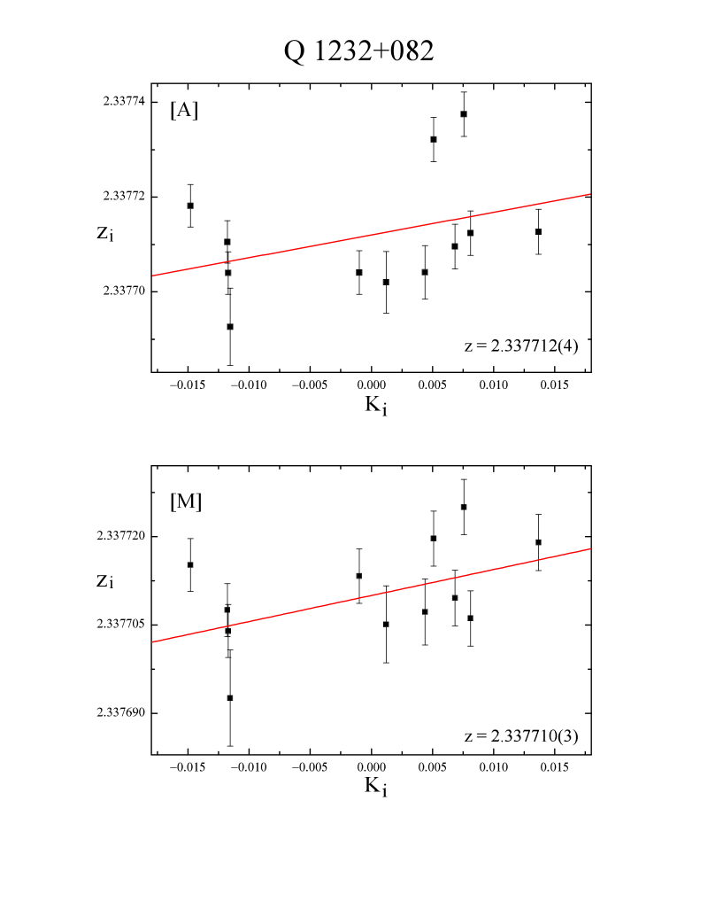
Figure 1:   Results of $z_{i}$-to-$K_{i}$ regression analysis for H₂ lines at $z_{abs}=2.3377$ in the Q 1232+082 spectrum. Upper panel: laboratory wavelengths are taken from Abgrall et al. (1993). Bottom panel: laboratory wavelengths are taken from Morton & Dinerstein (1976).

Absorption system of H₂ at z=2.3377 in the spectrum of Q 1232+082
More than 50 lines of molecular hydrogen (with S/N $\sim$ 10-14) are identified in the range 3400-3800 Å. We have carefully selected lines that are isolated, unsaturated and unblended. In this system only 12 lines meet all these conditions (see Table 1). The accuracy on the observed wavelengths $\lambda_{i}$ calculated in accordance with Eq. (A14) from Bohlin et al. (1983) which takes into account the number of points within the profile of the spectral line, the spectral resolution and the S/N ratio. The average uncertainty of the determination of the line centers is $\sigma(\lambda_{i})\sim 5$ mÅ. For the laboratory wavelengths we have used two independent sets of data: $\lambda_{i}^{0}\;[M]$ from Morton & Dinerstein, 1976; and $\lambda_{i}^{0}\;[A]$ from Abgrall et al., 1993 (see, also Roncin & Launay, 1994). Results of the linear regression analysis of $z_{i}$-to-$K_{i}$ are shown on Fig. 1 for both sets of laboratory wavelengths. They are the following: $\Delta\mu/\mu=(14.4\pm 11.4)\times 10^{-5}$ [A], and $\Delta\mu/\mu=(13.2\pm 7.4)\times 10^{-5}$ [M].

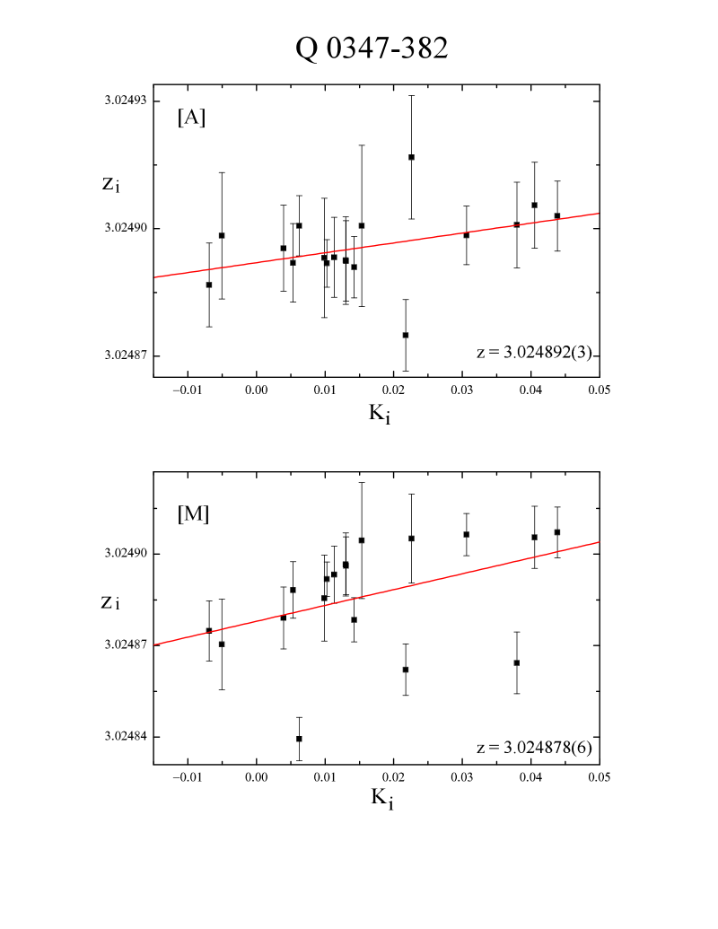
Figure 2:   Results of $z_{i}$-to-$K_{i}$ regression analysis for H₂ lines at $z_{abs}=3.0249$ in the Q 0347-382 spectrum. Upper panel: laboratory wavelengths are taken from Abgrall et al. (1993). Bottom panel: laboratory wavelengths are taken from Morton & Dinerstein (1976).

Absorption system of H₂ at z=3.0249 in the spectrum of Q 0347-382
For the first time, this H₂ system was found and investigated by Levshakov et al., 2001. More than 80 lines of molecular hydrogen (with S/N $\sim$ from 10 to 40) can be identified in the wavelength range 3600-4600 Å. We have reanalysed this spectrum independently. For our analysis 18 lines of H₂ were selected which satisfied to the conditions mentioned above. The average uncertainty of the determination of the line centers is $\sigma(\lambda_{i})\sim 10$ mÅ. Parameters of the lines are presented in Table 2. The results of the linear regression analysis of $z_{i}$-to-$K_{i}$ are shown on Fig. 2 for both sets of laboratory wavelengths. They are the following: $\Delta\mu/\mu=(5.8\pm 3.4)\times 10^{-5}$ [A], and $\Delta\mu/\mu=(12.2\pm 7.3)\times 10^{-5}$ [M]. It should be mention that three points on the bottom panel of Fig. 2 depart from the regression line more than $3\sigma$. Two of them corresponding to L 9-0 R(1) and W 1-0 R(1) transitions have the laboratory wavelengths marked by Morton & Dinerstein (1976) as a blended line and a line under weak continuum. The third point corresponding to W 3-0 Q(1) transition has deviations on the both panels. It may be a result of undetectable blending in the quasar spectrum. We do not reject these points because all of them satisfy to the above formulated conditions for the line selection from quasar spectra.

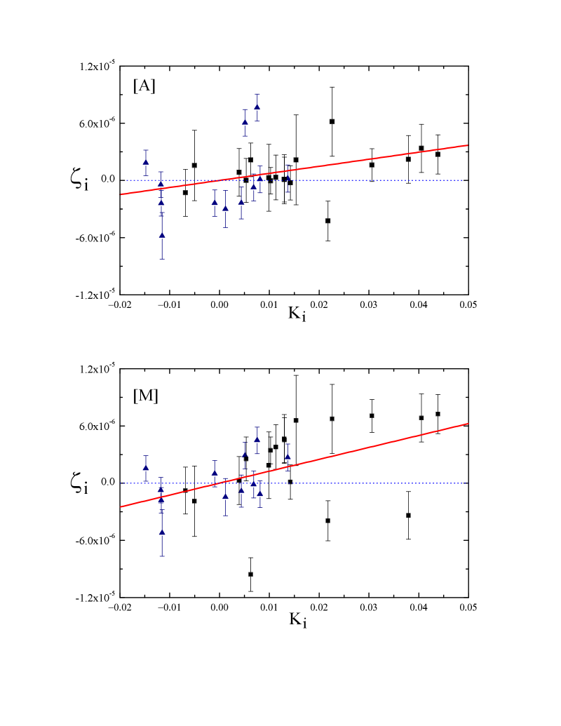
Figure 3:   Combined regression analysis of $\zeta_{i}$-to-$K_{i}$ for the systems at $z_{abs}=2.3377$ (triangles) and $3.0249$ (squares). Upper panel: laboratory wavelengths are taken from Abgrall et al. (1993). Bottom panel: laboratory wavelengths are taken from Morton & Dinerstein (1976).

Combined Analysis
The combined analysis of the H₂ lines from the two systems discussed above allows us to increase the statistical significance of the estimate because of increasing the number of lines involved and, what is more essential, broadening the interval of K-values. The results of linear regression analysis of $\zeta_{i}$ as a function of $K_{i}$ for all 30 lines from both systems are shown in Fig. 3. Here $\zeta_{i}$ is the reduced value of the line redshift:

$$\zeta_{i}=\frac{z_{i}-\overline{z}}{1+\overline{z}}\,,$$ (4)

where $\,\overline{z}\,$ is $z_{abs}$ corresponding to the absorption system and a particular set of laboratory wavelengths.

As a result of the combined analysis we obtained the following estimates (for two different sets of laboratory wavelengths):

$$\Delta\mu/\mu=(5.7\pm 3.8)\times 10^{-5}\;\;\;[A]\,,$$

$$\Delta\mu/\mu=(12.5\pm 4.5)\times 10^{-5}\;\;\;[M].$$

The statistical uncertainties of the laboratory wavelengths are about $1.5\,$mÅ  corresponding to an error of $\Delta\mu/\mu$ about $2\times 10^{-5}$ that is in agreement with the errors found from the regression.

Conclusions

The above results may be considered as a glimpse on possible cosmological variation of $\mu$. Additional measurements are necessary to ascertain the conclusion.

In any case, we have obtained the most stringent estimate on a possible cosmological variation of $\mu$ between redshift zero and redshifts 2–3.

In order to improve the result, it is necessary to measure more H₂ absorption systems at high redshift. The most suitable quasars for such analysis are PKS 0528-250, Q 0347-382, and Q 1232+082. Their observations with high resolution (FWHM $\sim 7$ km/s) and high S/N ratio ($>30$) will strengthen the conclusions.

In addition, better accuracy of laboratory wavelengths is also desirable because the contribution of laboratory statistical errors are comparable to the statistical errors of astronomical measurements.

Acknowledgments: The observations have been obtained with UVES mounted on the 8.2-m KUEYEN telescope operated by the European Southern Observatory at Parana, Chili. The authors thank C. Ledoux for primary reduction of the spectra and A. Potekhin for useful discussion. A. Ivanchik and D. Varshalovich are grateful for the support by the RFBR (01-02-06098, 99-02-18232). A. Ivanchik is grateful for the opportunity to visit the IAP CNRS.

References

Abgrall H., Roueff E., Launay F., Roncin J.-Y., Subtil J.-L. // Astron. Astrophys. Suppl. Ser., 1993, V. 101, P. 273.
Bohlin R.C., Hill J.K., Jenkins E.B., Savage B.D., Snow Jr. T.P., Spitzer Jr. L., York D.G. // Astrophys. J. Suppl. Ser., 1983, V. 51, P. 277.
Calmet X., Fritzsch H. // 2001, /hep-ph/0112110.
Damour T., Polyakov A.M. // Nucl. Phys., 1994, B423, P. 532.
D’Odorico S., Dessauges-Zavadsky M., Molaro P. // Astron. Astrophys., 2001, V. 368, P. L1.
Gasser J., Leutwyler H. // Physics Reports, 1982, V. 87, No. 3, P. 77.
Ivanchik A.V., Potekhin A.Y., Varshalovich D.A. // Astron. Astrophys., 1999, V. 343, P. 439.
Levshakov S.A., Dessauges-Zavadsky M., D’Odorico S., Molaro P. // Astrophys. J., 2002, V. 565, in press.
Mohr P.J, Taylor B.N. // Reviews of Modern Physics, 2000, V. 72, No. 2, P. 351.
Morton D.C., Dinerstein H.L. // Astrophys. J., 1976, V. 204, P. 1.
Petitjean P., Srianand R., Ledoux C. // 2000, /astro-ph/0011437.
Potekhin A.Y., Ivanchik A.V., Varshalovich D.A., Lanzetta K.M., Baldwin J.A., Williger G.M., Carswell R.F. // Astrophys. J., 1998, V. 505, P. 523.
Ronchin J.-Y., Launay F., // Journal Phys. and Chem. Reference Data, 1994, No. 4.
Varshalovich D.A., Levshakov S.A. // JETP Letters, 1993, V. 58, P. 231.
Varshalovich D.A., Potekhin A.Y. // Space Science Rev., 1995, V. 74, P. 259.
Vysotsky M.I., Novikov V.A., Okun’ L.B., Rozanov A.N. // Physics-Uspekhi, 1996, V. 166, No. 5, P. 539.
Webb J.K., Murphy M.T., Flambaum V.V., Dzuba V.A., Barrow J.D., Churchill C.W., Prochaska J.X., Wolfe A.M. // Phys. Rev. Lett., 2001, V. 87, P. 091301.

Table 1: H₂ lines of absorption system at $z_{abs}=2.3377$ in Q 1232+082 spectrum

$$\begin{array}[]{rrrrcr}\hline\cr\hline\cr\vskip 3.0pt plus 1.0pt minus 1.0pt\cr\mbox{Lines~{}~{}~{}~{}}&\;\;\;\;\lambda_{i}^{0},\,\mbox{\AA}\;[M]&\;\;\;\;\lambda_{i}^{0},\,\mbox{\AA}\;[A]&\;\;\;\;\lambda_{i},\,\mbox{\AA}&\sigma(\lambda_{i}),\,\mbox{\AA}&K_{i}\\ \vskip 3.0pt plus 1.0pt minus 1.0pt\cr\hline\cr\vskip 3.0pt plus 1.0pt minus 1.0pt\cr\mbox{L~{}0-0~{}P(3)}&1115.896&1115.895&3724.543&0.005&-0.01479\\ \mbox{L~{}0-0~{}R(3)}&1112.584&1112.583&3713.480&0.005&-0.01178\\ \mbox{L~{}0-0~{}P(2)}&1112.495&1112.459&3713.179&0.005&-0.01170\\ \mbox{L~{}1-0~{}P(4)}&1104.084&1104.084&3685.093&0.009&-0.01154\\ \mbox{L~{}2-0~{}P(3)}&1084.559&1084.562&3619.947&0.005&-0.00098\\ \mbox{L~{}3-0~{}P(4)}&1074.313&1074.314&3585.740&0.007&0.00122\\ \mbox{L~{}3-0~{}R(4)}&1070.898&1070.899&3574.344&0.006&0.00439\\ \mbox{L~{}3-0~{}P(3)}&1070.142&1070.138&3571.834&0.005&0.00511\\ \mbox{L~{}3-0~{}R(3)}&1067.478&1067.474&3562.948&0.005&0.00758\\ \mbox{L~{}3-0~{}P(2)}&1066.901&1066.899&3561.002&0.005&0.00812\\ \mbox{L~{}4-0~{}P(4)}&1060.580&1060.580&3539.908&0.005&0.00685\\ \mbox{L~{}4-0~{}P(2)}&1053.281&1053.283&3515.556&0.005&0.01369\\ \vskip 3.0pt plus 1.0pt minus 1.0pt\cr\hline\cr\end{array}$$

Table 2: H₂ lines of absorption system at $z_{abs}=3.0249$ in Q 0347-382 spectrum

$$\begin{array}[]{rrrrcr}\hline\cr\hline\cr\vskip 3.0pt plus 1.0pt minus 1.0pt\cr\mbox{Lines~{}~{}~{}~{}}&\;\;\;\;\lambda_{i}^{0},\,\mbox{\AA}\;[M]&\;\;\;\;\lambda_{i}^{0},\,\mbox{\AA}\;[A]&\;\;\;\;\lambda_{i},\,\mbox{\AA}&\sigma(\lambda_{i}),\,\mbox{\AA}&K_{i}\\ \vskip 3.0pt plus 1.0pt minus 1.0pt\cr\hline\cr\vskip 3.0pt plus 1.0pt minus 1.0pt\cr\mbox{L~{}~{}2-0~{}R(1)}&1077.698&1077.697&4337.614&0.010&0.00535\\ \mbox{L~{}~{}3-0~{}R(2)}&1064.995&1064.993&4286.483&0.015&0.00989\\ \mbox{L~{}~{}3-0~{}P(1)}&1064.606&1064.606&4284.924&0.006&0.01026\\ \mbox{L~{}~{}3-0~{}R(1)}&1063.460&1063.460&4280.313&0.010&0.01132\\ \mbox{L~{}~{}4-0~{}R(3)}&1053.976&1053.977&4242.144&0.010&0.01304\\ \mbox{L~{}~{}4-0~{}R(2)}&1051.497&1051.498&4232.175&0.020&0.01536\\ \mbox{L~{}~{}6-0~{}R(3)}&1028.986&1028.983&4141.571&0.015&0.02262\\ \mbox{L~{}~{}7-0~{}R(1)}&1013.434&1013.436&4078.977&0.007&0.03062\\ \mbox{W~{}~{}0-0~{}Q(2)}&1010.941&1010.938&4068.911&0.010&-0.00686\\ \mbox{W~{}~{}0-0~{}R(2)}&1009.030&1009.023&4061.215&0.015&-0.00503\\ \mbox{L~{}~{}9-0~{}R(1)}&992.022&992.013&3992.754&0.010&0.03796\\ \mbox{W~{}~{}1-0~{}Q(2)}&987.978&987.974&3976.492&0.010&0.00394\\ \mbox{W~{}~{}1-0~{}R(1)}&985.651&985.636&3967.087&0.007&0.00626\\ \mbox{L~{}10-0~{}P(1)}&982.834&982.834&3955.814&0.010&0.04053\\ \mbox{L~{}12-0~{}R(3)}&967.674&967.675&3894.798&0.008&0.04386\\ \mbox{W~{}~{}2-0~{}Q(2)}&967.278&967.279&3893.194&0.010&0.01301\\ \mbox{W~{}~{}2-0~{}Q(1)}&966.097&966.094&3888.423&0.007&0.01423\\ \mbox{W~{}~{}3-0~{}Q(1)}&947.425&947.422&3813.255&0.008&0.02176\\ \vskip 3.0pt plus 1.0pt minus 1.0pt\cr\hline\cr\end{array}$$