The 2dF Galaxy Redshift Survey: The amplitudes of fluctuations in the 2dFGRS and the CMB, and implications for galaxy biasing

Abstract

We compare the amplitudes of fluctuations probed by the 2dF Galaxy Redshift Survey and by the latest measurements of the Cosmic Microwave Background anisotropies. By combining the 2dFGRS and CMB data we find the linear-theory rms mass fluctuations in $8{\,h^{-1}\,{\rm Mpc}}$ spheres to be $\sigma_{8{\rm m}}=0.73\pm 0.05$ (after marginalization over the matter density parameter ${\Omega_{\rm m}}$ and three other free parameters). This normalization is lower than the COBE normalization and previous estimates from cluster abundance, but it is in agreement with some revised cluster abundance determinations. We also estimate the scale-independent bias parameter of present-epoch $L_{s}=1.9L_{*}$ APM-selected galaxies to be $b(L_{s},z=0)=1.10\pm 0.08$ on comoving scales of $0.02<k<0.15{\,h\,\rm Mpc^{-1}}$. If luminosity segregation operates on these scales, $L_{*}$ galaxies would be almost un-biased, $b(L_{*},z=0)\approx 0.96$. These results are derived by assuming a flat $\Lambda$CDM Universe, and by marginalizing over other free parameters and fixing the spectral index $n=1$ and the optical depth due to reionization $\tau=0$. We also study the best fit pair $({\Omega_{\rm m}},b)$, and the robustness of the results to varying $n$ and $\tau$. Various modelling corrections can each change the resulting $b$ by 5–15 per cent. The results are compared with other independent measurements from the 2dFGRS itself, and from the SDSS, cluster abundance and cosmic shear. Key words: Cosmology, CMB, galaxies, Statistics

1 Introduction

The 2dF Galaxy Redshift Survey (2dFGRS) has now measured over 210 000 galaxy redshifts and is the largest existing galaxy redshift survey (Colless et al. 2001). A sample of this size allows large-scale structure statistics to be measured with very small random errors. Two other 2dFGRS papers, Percival et al. (2001; hereafter P01) and Efstathiou et al. (2001; hereafter E02) have mainly compared the shape of the 2dFGRS and CMB power spectra, and concluded that they are consistent with each other (see also Tegmark, Hamilton & Xu 2001). Here we estimate the amplitudes of the rms fluctuations in mass $\sigma_{8{\rm m}}$ and in galaxies $\sigma_{8{\rm g}}$. More precisely, we consider the ratio of galaxy to matter power spectra, and use the ratio of these to define the bias parameter:

$$b^{2}\equiv{P_{\rm{gg}}(k)\over P_{\rm{mm}}(k)}.$$ (1)

As defined here, $b$ is in principle a function of scale. In practice, we will measure the average value over the range of wavenumbers $0.02<k<0.15{\,h\,\rm Mpc^{-1}}$. On these scales, the fluctuations are close to the linear regime, and there are good reasons (e.g. Benson et al. 2000) to expect that $b$ should tend to a constant. In this study, we will not test the assumption that the biasing is scale-independent, but we do allow it to be function of luminosity and redshift.

A simultaneous analysis of the constraints placed on cosmological parameters by different kinds of data is essential because each probe – e.g. CMB, Type Ia supernovae (SNe Ia), redshift surveys, cluster abundance, and peculiar velocities – typically constrains a different combination of parameters (e.g. Bahcall et al. 1999; Bridle et al. 2000, 2001a; E02). A particular case of joint analysis is that of galaxy redshift surveys and the Cosmic Microwave Background (CMB). While the CMB probes the fluctuations in matter, the galaxy redshift surveys measure the perturbations in the light distribution of particular tracer (e.g. galaxies of certain type). Therefore, for a fixed set of cosmological parameters, a combination of the two can tell us about the way galaxies are ‘biased’ relative to the mass fluctuations (e.g. Webster et al. 1998).

A well-known problem in estimating cosmological parameters is the degeneracy of parameters, and the choice of free parameters. Here we consider three classes of parameters:

(i) Parameters that are fixed by theoretical assumptions or prejudice (which may be supported by observational evidence). Here we assume a flat Universe (i.e. zero curvature), and no tensor component in the CMB (for discussion of the degeneracy with respect to these parameters see E02).

(ii) The ‘free parameters’ that are of interest to address a particular question. For the joint 2dFGRS & CMB analysis presented here we consider five free parameters: the matter density parameter ${\Omega_{\rm m}}$, the linear-theory amplitude of the mass fluctuations $\sigma_{8{\rm m}}$, the present-epoch linear biasing parameter $b(L_{s},z=0)$ (for the survey effective luminosity $L_{s}\simeq 1.9L_{*}$), the Hubble constant $h\equiv H_{0}/(100{\,\rm km\,s^{-1}})$, and the baryon density parameter $\omega_{\rm b}\equiv{\Omega_{\rm b}}h^{2}$. As we are mainly interested in combinations of $\sigma_{8{\rm m}}$, $b$ and ${\Omega_{\rm m}}$, we shall marginalize over the remaining parameters.

(iii) The robustness of the results to some ‘extra parameters’, that are uncertain. Here we consider the optical depth $\tau$ due to reionization (see below) and the primordial spectral index $n$. We use as our canonical values $\tau=0$ and $n=1$, but we also quote the results for other possibly realistic values, $\tau=(0.05,0.2)$ and $n=(0.9,1.1)$.

The outline of this paper is as follows. In Section 2 we derive $\sigma_{8{\rm g}}$ from the 2dFGRS alone, taking into account corrections for redshift-space distortion and for epoch-dependent and luminosity-dependent biasing. In Section 3 we derive $\sigma_{8{\rm m}}$ from the latest CMB data. In Section 4 we present a joint analysis of 2dFGRS & CMB. Finally, in Section 5 we compare and contrast our measurements with other cosmic probes.

2 The amplitude of the 2dFGRS fluctuations

2.1 $\bf\sigma^{\bf S}_{\bf 8{\rm g}}$ from the fitted power spectrum

An initial estimate of the convolved, redshift-space power spectrum of the 2dFGRS has already been determined (P01), using the Fourier-transform-based technique described by Feldman, Kaiser & Peacock (1994; hereafter FKP) for a sample of 160 000 redshifts. On scales $0.02<k<0.15{\,h\,\rm Mpc^{-1}}$, the data are robust and the shape of the power spectrum is not affected by redshift-space or non-linear effects, though the amplitude is increased by redshift-space distortions (see later). We use the resulting power spectrum from P01 in this paper to constrain the amplitude of the fluctuations.

As explained above, we define the bias parameter as the square root of the ratio of the galaxy and mass power spectra on large scales. We shall assume that the mass power spectrum can be described by a member of the family of models dominated by Cold Dark Matter (CDM). Such models traditionally have their normalization described by the linear-theory value of the rms fractional fluctuations in density averaged in spheres of $8{\,h^{-1}\,{\rm Mpc}}$ radius: $\sigma_{8{\rm m}}$. It is therefore convenient to define a corresponding measure for the galaxies, $\sigma_{8{\rm g}}$, such that we can express the bias parameter as

$$b={\sigma_{8{\rm g}}\over\sigma_{8{\rm m}}}.$$ (2)

The scale of $8{\,h^{-1}\,{\rm Mpc}}$ was chosen historically because $\sigma_{8{\rm g}}\sim 1$ from the optically-selected Lick counts (Peebles 1980), so it may seem impossible by definition to produce a linear-theory $\sigma_{8}$ for galaxies. In practice, we define $\sigma_{8{\rm g}}$ to be the value required to fit a CDM model to the power-spectrum data on linear scales ($0.02<k<0.15{\,h\,\rm Mpc^{-1}}$). From this point of view, one might equally well specify the normalization via e.g. $\sigma_{20}$; however, the $\sigma_{8}$ parameter is more familiar in the context of CDM models. The regions of the power spectrum that generate the $\sigma_{8}$ signal are at only slightly higher $k$ than our maximum value, so no significant uncertainty arises from extrapolation. A final necessary complication of the notation is that we need to distinguish between the apparent values of $\sigma_{8{\rm g}}$ as measured in redshift space ($\sigma_{8{\rm g}}^{S}$) and the real-space value that would be measured in the absence of redshift-space distortions ($\sigma_{8{\rm g}}^{R}$). It is the latter value that is required in order to estimate the bias.

Figure 1: The observed (i.e. convolved with the window function) 2dFGRS power spectrum (as derived in P01). The solid line shows a linear theory $\Lambda$CDM fit (convolved with the window function) with ${\Omega_{\rm m}}h=0.2,{\Omega_{\rm b}}/{\Omega_{\rm m}}=0.15,h=0.7,n=1$ and best-fitting $\sigma^{S}_{8{\rm g}}(z_{s},L_{s})=0.94$. Only the range $0.02<k<0.15{\,h\,\rm Mpc^{-1}}$ is used at the present analysis (roughly corresponding to CMB harmonics $200<\ell<1500$ in a flat ${\Omega_{\rm m}}=0.3$ Universe). The good fit of the linear theory power spectrum at $k>0.15{\,h\,\rm Mpc^{-1}}$ is due to a conspiracy between the non-linear growth and finger-of-god smearing (integrating over the observed $P(k)$ therefore provides another way of estimating the normalization, giving $\sigma^{S}_{8{\rm g}}\simeq 0.95$).

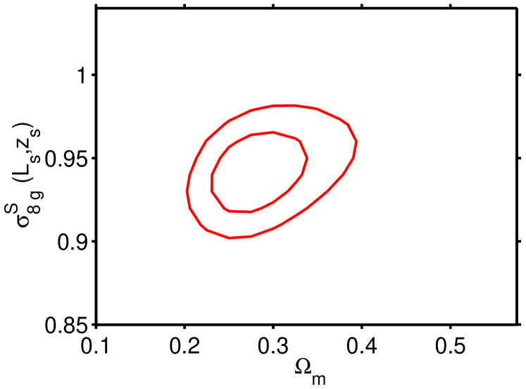
Figure 2: The likelihood function of 2dFGRS as a function of of the galaxy fluctuation amplitude in redshift space $\sigma^{S}_{8{\rm g}}(L_{s},z_{s})$ and the present epoch ${\Omega_{\rm m}}$. The marginalization over the Hubble constant is done with a Gaussian centred at $h=0.7$ and standard deviation of 0.07. Other parameters are held fixed ($n=1,\omega_{\rm b}=0.02$). The contours contain 68 per cent and 95 per cent of the probability.

The 2dFGRS power spectrum (Fig. 1) is fitted in P01 over the above range in $k$, assuming scale-invariant primordial fluctuations and a $\Lambda$CDM cosmology, for four free parameters: ${\Omega_{\rm m}}h$, ${\Omega_{\rm b}}/{\Omega_{\rm m}}$, $h$ and the redshift space $\sigma^{S}_{8{\rm g}}$ (using the transfer function fitting formulae of Eisenstein & Hu 1998) . Assuming a Gaussian prior on the Hubble constant $h=0.7\pm 0.07$ (based on Freedman et al. 2001) the shape of the recovered spectrum within the above $k$-range was used to yield 68 per cent confidence limits on the shape parameter ${\Omega_{\rm m}}h=0.20\pm 0.03$, and the baryon fraction ${\Omega_{\rm b}}/{\Omega_{\rm m}}=0.15\pm 0.07$, in accordance with the popular ‘concordance’ model. Although the $\Lambda$CDM model with comparable amounts of dark matter and dark energy is rather esoteric, it is remarkable that the 2dFGRS measurement shows such good consistency with other cosmological probes such as CMB, SNe, and Big Bang Nucleosynthesis (BBN).

We find that $\sigma^{S}_{8{\rm g}}$ depends only weakly on the other three parameters, with the strongest correlation with ${\Omega_{\rm m}}$. For fixed ‘concordance model’ parameters $n=1,{\Omega_{\rm m}}=1-{\Omega_{\Lambda}}=0.3$, $\omega_{\rm b}=0.02$ and a Hubble constant $h=0.70$, we find that the amplitude of 2dFGRS galaxies in redshift space is $\sigma_{8{\rm g}}^{S}(L_{s},z_{s})=0.94$ (when all other parameters are held fixed, the formal errors are unrealistically tiny, only a few percent, and hence we do not quote them). In the FKP method, the normalization of the power spectrum depends on the radial number density and weighting function, and a number of different methods have been suggested for calculating the normalization (Sutherland et al. 1999) using a random catalogue designed to Poisson sample the survey region. P01 tried all of the suggested methods for the 2dFGRS data and found no significant change in the power spectrum normalization. Therefore, although this calculation remains a potential cause of systematic error in the power-spectrum normalization, we shall assume hereafter that the main uncertainty in the derived bias derives from the uncertain cosmological model that is needed in order to connect the galaxy power spectrum with the mass power spectrum from the CMB.

On keeping ${\Omega_{\rm m}}$ free and marginalizing over $h$ with a Gaussian prior (with $h=0.7\pm 10$ per cent) we obtain Fig. 2. The external constraint on $h$ that we impose translates to a constraint on ${\Omega_{\rm m}}$ through the 2dFGRS sensitivity to the matter power spectrum shape, which is roughly ${\Omega_{\rm m}}h$. On marginalizing over ${\Omega_{\rm m}}$ we find $\sigma^{S}_{8{\rm g}}=0.94\pm 0.02$, in agreement with the best-fit non-marginalized result.

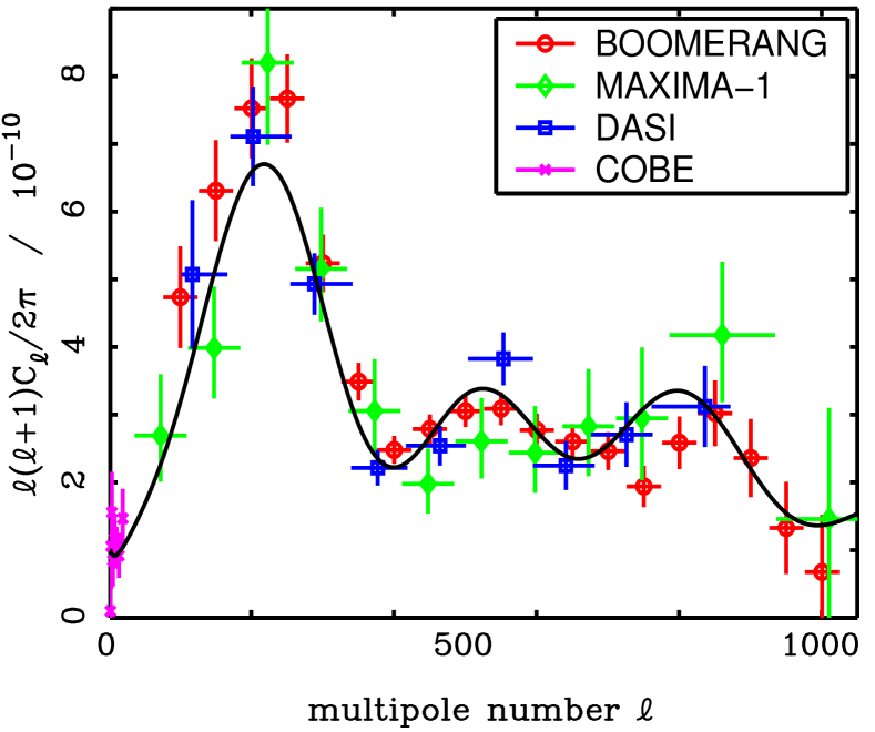
Figure 3: A compilation of the latest CMB data points from COBE, Boomerang, Maxima and DASI against spherical harmonic $\ell$. The line shows the predicted angular power spectrum for a $\Lambda$CDM model with $n=1$, ${\Omega_{\rm m}}=1-\Omega_{\Lambda}=0.3$, $\omega_{\rm b}=0.02$ (BBN value), $h=0.70$, $\tau=0.0$, and the best-fit normalization to the given CMB data points $\sigma_{8{\rm m}}=0.83$. Note that this normalization is lower than the traditional COBE-only normalization (see Table 1). A similar model is also the best fit to the shape of the 2dFGRS galaxy power spectrum (Fig. 1).

2.2 Corrections for redshift and luminosity effects

In reality, the effective redshift for the P01 analysis is not zero, but $z_{s}\sim 0.17$. This is higher than the median redshift of 2dFGRS ($z_{m}\sim 0.11$) due to the weighting scheme used in estimating the power spectrum. Similarly, $L_{s}\simeq 1.9L_{*}$, rather than the $L_{s}\simeq L_{*}$ that would apply for a flux-limited sample. We can then derive $\sigma^{S}_{8{\rm g}}(L_{s},z_{s})$ directly, but for comparison with other studies we make further steps of calculating $\sigma^{R}_{8{\rm g}}(L_{s},z=0)$ and then $\sigma^{R}_{8{\rm g}}(L_{*},z=0)$. This requires corrections which depend on the nature of galaxy formation and on clustering with redshift. Some of the corrections themselves depend on cosmological parameters, and our procedure solves for the best-fitting values in a self-consistent way.

We start by evaluating the conversion from redshift space to real space at the survey effective redshift $z_{s}$ for galaxies with effective luminosity $L_{s}$:

$$\sigma_{8{\rm g}}^{R}(L_{s},z_{s})=\sigma_{8{\rm g}}^{S}(L_{s},z_{s})/K^{1/2}[\beta(L_{s},z_{s})]\;\;.$$ (3)

where

$$K[\beta]=1+{\frac{2}{3}}\beta+{\frac{1}{5}}\beta^{2}$$ (4)

is Kaiser’s (1987) factor, derived in linear theory and the distant-observer approximation. The dependence of $\beta$ on redshift can be written as:

$$\beta(L_{s},z_{s})\simeq{\Omega_{\rm m}}^{0.6}(z_{s})/b(L_{s},z_{s}),$$ (5)

assuming linear biasing [for more general biasing schemes see e.g. Dekel & Lahav (1999) and references therein].

The evolution of the matter density parameter with redshift is

$${\Omega_{\rm m}}(z)={\Omega_{\rm m}}\;(1+z)^{3}\;(H/H_{0})^{-2}$$ (6)

with

$$(H/H_{0})^{2}=[{\Omega_{\rm m}}(1+z)^{3}+(1-{\Omega_{\rm m}}-{\Omega_{\Lambda}})(1+z)^{2}+{\Omega_{\Lambda}}]\;.$$ (7)

The variation of $b(z)=\sigma_{8{\rm g}}(z)/\sigma_{8{\rm m}}(z)$ with redshift is even more model-dependent. We assume that the mass fluctuations grow as $\sigma_{8{\rm m}}(z)=\sigma_{8{\rm m}}(0)D(z)$, where $D(z)$ (normalized to 1 at $z=0$) is the growing mode of fluctuations in linear theory [it depends on ${\Omega_{\rm m}}$ and ${\Omega_{\Lambda}}$, e.g. Peebles (1980)].

We also assume that galaxy clustering weakly evolves over $0<z<0.2$, i.e. $\sigma_{8{\rm g}}(L_{s},0)\simeq\sigma_{8{\rm g}}(L_{s},z)$. We shall refer to this simple model as the ‘constant galaxy clustering (CGC) model’. Simulations suggest (e.g. Kauffmann et al. 1999; Blanton et al. 2000; Benson et al. 2000; Somerville et al. 2001) that even if the clustering of dark matter halos evolves slightly over this range of redshifts, galaxy clustering evolves much less. Indeed, observationally there is only a weak evolution of clustering of the overall galaxy population over the redshift range $0.1<z<0.5$ (e.g. the CNOC2 survey: Shepherd et al. 2001). Therefore in our simple CGC model (for any luminosity):

$$b(L_{s},z_{s})=b(L_{s},0)/D(z_{s}).$$ (8)

There are of course other possible models for the evolution of galaxy clustering with redshift, e.g. the galaxy conserving model (Fry 1996). This model describes the evolution of bias for test particles by assuming that they follow the cosmic flow. It can be written as:

$$b(L_{s},z_{s})=1+[b(L_{s},0)-1]/D(z_{s}).$$ (9)

More elaborate models exist, such as those based on a merging model (e.g. Mo & White 1996; Matarrese et al. 1997; Magliocchetti et al. 1999) or numerical and semi-analytic models (Benson et al. 2000; Somerville et al. 2001).

To estimate the magnitude of these effects we consider the 2dFGRS effective redshift $z_{s}=0.17$. For a Universe with present-epoch ${\Omega_{\rm m}}=0.3$ and ${\Omega_{\Lambda}}=0.7$ we get ${\Omega_{\rm m}}(z_{s})=0.41$ and $D(z_{s})=0.916$, hence for the CGC model with ${\Omega_{\rm m}}=0.3$, $b(L_{s},z_{s})=1.09\;b(L_{s},0)$ and $\beta(L_{s},z_{s})=1.10\;\beta(L_{s},0)$.

On the other hand, we can also relate the amplitude of galaxy clustering to the present-epoch mass fluctuations $\sigma_{8{\rm m}}$, which can be estimated from the CMB (see below):

$$\sigma_{8{\rm g}}^{R}(L_{s},0)=b(L_{s},0)\sigma_{8{\rm m}}(0)\;.$$ (10)

Hence by combining equations (3), (8) and (10) we can solve for $b(L_{s},0)$.

Finally, there is the issue of luminosity-dependent biasing. Although controversial for some while, this effect has now been precisely measured by the 2dFGRS (Norberg et al. 2001a,2002); see also recent results from the SDSS (Zehavi et al. 2001). Norberg et al. (2001a) found from correlation-function analysis that on scales $\lower 2.15277pt\hbox{$\;\buildrel<\over{\sim}\;$}10{\,h^{-1}\,{\rm Mpc}}$

$$b(L,0)/b(L_{*},0)=0.85+0.15(L/L_{*})\;.$$ (11)

If we assume that this relation also applies in the linear regime probed by our $P(k)$ on scales $0.02<k<0.15{\,h\,\rm Mpc^{-1}}$, then the linear biasing factor for $L_{*}$ galaxies at redshift zero is 1.14 smaller then that for the 2dFGRS galaxies with effective survey luminosity $L_{s}=1.9L_{*}$ ($K$-corrected). However, this is a source of uncertainty, and ultimately it can be answered with the complete 2dFGRS and SDSS surveys by calculating the power spectra in luminosity bins.

The luminosities in equation (11) have been $K$-corrected and also corrected for passive evolution of the stellar populations, but the clustering has been measured at various median redshifts (for galaxies at the redshift range $0.02<z<0.28$). Possible variation of galaxy clustering with redshift is still within measurement errors of Norberg et al. (2001a,2002). For simplicity we shall assume in accord with our CGC model that this relation is redshift-independent over the redshift range of 2dFGRS ($z\la 0.2$). We see that the effects of redshift-space distortion and luminosity bias are quite significant, at the level of more than $10$ per cent each.

3 The CMB data

The CMB fluctuations are commonly represented by the spherical harmonics $C_{\ell}$. The connection between the harmonic $\ell$ and $k$ is roughly

$$\ell\simeq k\,d_{A}$$ (12)

where for a flat Universe the angular distance to the last scattering surface is well approximated by (Vittorio & Silk 1991):

$$d_{A}\simeq{\frac{2c}{H_{0}\,\Omega_{\rm m}^{0.4}}}\;.$$ (13)

For ${\Omega_{\rm m}}=0.3$ the 2dFGRS range $0.02<k<0.15{\,h\,\rm Mpc^{-1}}$ corresponds approximately to $200<\ell<1500$, which is well covered by the recent CMB experiments. We obtain theoretical CMB power spectra using the CMBFAST code (Seljak & Zaldarriaga 1996).

The latest CMB measurements from Boomerang (Netterfield et al. 2001, de Bernardis et al. 2002), Maxima (Lee et al. 2001; Stomper et al. 2001) and DASI (Halverson et al. 2002; Pryke et al. 2002) suggest three acoustic peaks. Parameter fitting to a $\Lambda$CDM model indicates consistency between the different experiments, and a best-fit Universe with zero curvature, and an initial spectrum with spectral index $n\simeq 1$ (e.g. Wang, Tegmark & Zaldriaga  2001, hereafter WTZ; E02 and references therein). Unlike the earlier Boomerang and Maxima results, the new data also show that the baryon contribution is consistent with the Big Bang Nucleosynthesis value $\omega_{\rm b}\simeq 0.02$ (O’Meara et al. 2001).

Various CMB data sets can be combined in different ways (e.g. Jaffe et al. 2001; Lahav et al. 2000). Here we consider two compilations of CMB data:

(a) a compilation of COBE (8 points), Boomerang, Maxima and DASI (hereafter CBMD). The total number of data points in this compilation is 49, plotted in Fig. 3.

(b) a compilation of 24 $\Delta T/T$ data points from Wang et al. (2001; WTZ), which is based on 105 band-power measurements of almost all available CMB experiments (including the latest Boomerang, Maxima, and DASI data).

Both compilations take into account the calibration errors, which are crucial for estimating the amplitude of fluctuations. For our compilation (a) we use a fast method for marginalization over calibration and beam uncertainties that assumes a Gaussian prior on the calibration and beam corrections (Bridle et al. 2001b). We apply the usual multi-variate $\chi^{2}$ procedure (e.g. Hancock et al. 1998), taking into account the window functions and the covariance matrix (when available). Since the Boomerang and Maxima window functions and correlation matrices are not yet available, we assume that the data points are uncorrelated and use top-hat window functions (as did WTZ). This assumption is validated by the fact that we obtain sensible values of $\chi^{2}$ for the best-fitting models.

3.1 CMB-only fits

We first consider the constraints arising from the CMB data alone. Table 1 summarizes various estimates for $\sigma_{8{\rm m}}$ from the above two new data sets. Note that these differ from the normalization returned by CMBFAST when only the COBE data are considered. This Table also illustrates the sensitivity of the results to the optical depth to reionization $\tau$ (see below). We see that differences in data sets and in assumptions on other parameters can easily lead to uncertainties of $\sim 10$ per cent in the resulting $\sigma_{8{\rm m}}$. Note that the normalizations derived from WTZ are lower than those derived from our compilation. This reflects that fact that WTZ chose to adjust downwards the calibrations of the principal datasets that we prefer to adopt. We incorporate the calibration uncertainties, but make no such adjustment.

Table 1: Normalizations for matter fluctuations derived by fitting to CMB data alone. In all the entries (unless otherwise stated) other parameters are fixed at ${\Omega_{\rm m}}=1-{\Omega_{\Lambda}}=0.3$, $\omega_{\rm b}=0.02$, $n=1$ and $h=0.7$. The first three entries were derived via CMBFAST using the COBE points according to the normalization procedure of Bunn & White (1996). The other entries were derived by the best fit multi-variate $\chi^{2}$ (including the covariance matrix and window functions) for the WTZ and CBMD data points (the goodness of fit is e.g. $\chi^{2}=35$ for 24 points in the fourth entry). Quoted error bars are 1-sigma. In some cases formal errors are not quoted as they are unrealistically tiny (few percent) when other parameters are held fixed. Note that both the WTZ and CBMD compilations give normalization lower than the COBE-only normalization.

Data	$\sigma_{8{\rm m}}$
COBE ($\tau=0$),	$0.90$
COBE ($\tau=0.05$),	$0.93$
COBE ($\tau=0.20$),	$0.98$
WTZ ($\tau=0$),	$0.77$
WTZ ($\tau=0.05$),	$0.80$
WTZ ($\tau=0.20$),	$0.92$
CBMD ($\tau=0$)	$0.83$
CBMD($\tau=0$, marg. over $h=0.7\pm 0.07$ )	$0.71\pm 0.07$
CBMD ($\tau=0$, marg. over $h=0.7\pm 0.07$ & ${\Omega_{\rm m}}$)	$0.68\pm 0.07$
CBMD ($\tau=0$) + 2dF, marg. over $h$, ${\Omega_{\rm m}}$, $\omega_{b}$ & $b$	$0.73\pm 0.05$

Fig. 4 (dashed lines) shows the likelihood as a function of $({\Omega_{\rm m}},\sigma_{8{\rm m}})$ after marginalization over the Hubble constant is done with a Gaussian with $h=0.7\pm 0.07$, while keeping other parameters fixed ($n=1,\omega_{\rm b}=0.02,\tau=0.0$). We note that for a fixed ${\Omega_{\rm m}}=0.3$ on this diagram the resulting $\sigma_{8{\rm m}}\sim 0.7$ is lower that the value we obtained above ($\sigma_{8{\rm m}}\sim 0.8$) when fixing the Hubble constant $h=0.7$ and other parameters. This illustrates the sensitivity of the results from the CMB alone to the Hubble constant. The external constraint on $h$ we have imposed cuts off the contours at low and high ${\Omega_{\rm m}}$. This is due to the constraint on ${\Omega_{\rm m}}h^{2}$ that exists from CMB data: a constraint on $h$ thus translates to a constraint on ${\Omega_{\rm m}}$. Completing the marginalization over ${\Omega_{\rm m}}$ we find $\sigma_{8{\rm m}}=0.68\pm 0.07$. Note that since we assume that the Universe is flat, there are additional constraints on our free parameters that come from the position of the first acoustic peak that make our error bars slightly smaller than studies that marginalize over the curvature of the Universe as well. We overlay in Fig. 4 the constraints from cluster abundance obtained recently by various authors. The cluster abundance constraint is fortunately orthogonal to the CMB constraint, but the spread in normalization values is quite large. It is interesting that some of the latest estimates are in good agreement with our estimates from the CMB and 2dFGRS+CMB (see further discussion below).

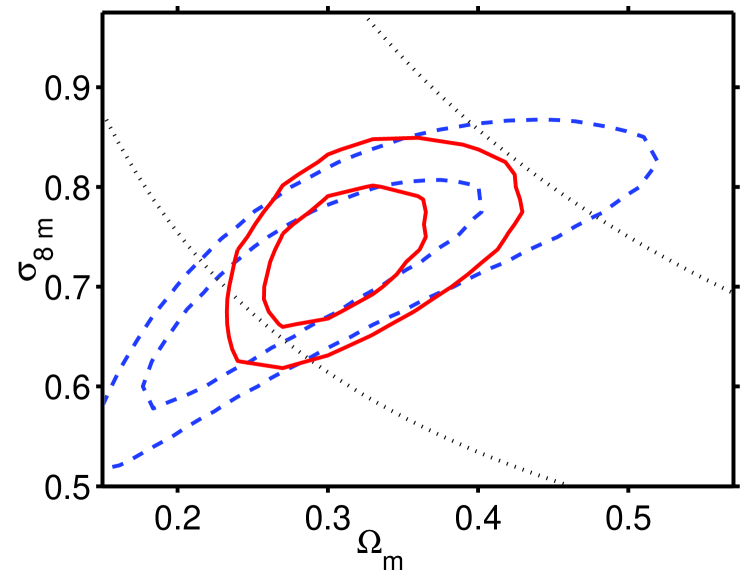
Figure 4: The likelihood function of CMB alone (dashed lines) in terms of the mass fluctuation amplitude $\sigma_{8{\rm m}}$ and the present epoch ${\Omega_{\rm m}}$. The marginalization over the Hubble constant is done with a Gaussian centred at $h=0.7$ and standard deviation of 0.07. Other parameters are held fixed ($n=1,\omega_{\rm b}=0.02,\tau=0.0$). The contours are for (two-parameter) 68 per cent and 95 per cent confidence intervals. The solid lines show the contours (68 per cent and 95 per cent) for the joint 2dFGRS&CMB analysis, after marginalization over $h$, $b(L_{s},0)$ and $\omega_{\rm b}$. Other parameters are held fixed ($n=1,\tau=0.0$). Note that the contours of 2dFGRS & CMB are much tighter than when using CMB alone. Two recent extreme cluster abundance determinations are overlayed as the upper dotted line (Pierpaoli et al. 2001) and the lower dotted line (Viana et al. 2002).

4 Combining 2dFGRS & CMB

When combining 2dFGRS and CMB data the parameterisation for the log-likelihoods is in five parameters:

 

$${{\ln{\mathcal{L}}}_{\rm tot}}$$

  (14)

where ${\mathcal{L}}_{\rm 2dFGRS}$ and ${\mathcal{L}}_{\rm CMB}$ are the likelihood functions for 2dFGRS and the CMB.

The 2dFGRS likelihood function takes into account the redshift-space distortions, the CGC biasing scheme, and the redshift evolution of ${\Omega_{\rm m}}(z)$. Here we use our compilation of 49 CMB data points (shown in Fig. 3). Other parameters are held fixed ($n=1,\tau=0$).

Fig.  4 (solid lines) shows the 2dFGRS+CMB likelihood as a function of $({\Omega_{\rm m}},\sigma_{8{\rm m}})$, after marginalization over $h,b(L_{s},0)$ and $\omega_{\rm b}$. The peak of the distribution is consistent with the result for the CMB alone (shown by the dashed lines in Fig.  4), but we see that the contours are tighter due to the addition of the 2dFGRS data. Further marginalization over ${\Omega_{\rm m}}$ gives $\sigma_{8{\rm m}}=0.73\pm 0.05$. The importance of adding the shape information of the 2dFGRS power spectrum is that it requires no external prior for $h$ and $\omega_{\rm b}$, unlike deriving $\sigma_{8{\rm m}}$ from CMB alone (Table 1). Our result is very similar to the value $\sigma_{8{\rm m}}\simeq 0.72$ derived in E02 using the WTZ data set and after marginalizing over the raw 2dFGRS amplitude of the power spectrum and other parameters.

To study the biasing parameter we marginalize the 2dFGRS likelihood over $h,\omega_{\rm b}$ and $\sigma_{8{\rm m}}$. Other parameters are held fixed ($n=1,\tau=0$). The resulting likelihood as a function of $[{\Omega_{\rm m}},b(L_{s},0)]$ is shown (by solid contours) in Fig. 5. Further marginalizing over ${\Omega_{\rm m}}$ gives $b(L_{s},0)=1.10\pm 0.08$ (1-sigma). With Fry’s biasing scheme (equation 9) $b(L_{s},0)$ is increased by $8$ per cent.

The effect of changing the spectral index to $n=0.9$ is shown (by dashed lines) in Fig. 5 (with $\tau=0$). Results for $n=0.9$ and $n=1.1$ with further marginalization over ${\Omega_{\rm m}}$ are given in Table 2, showing that $b(L_{s},0)$ is slightly down and up respectively relative to the standard $n=1$ case. We see that when we fit CMB data over a wide range of $\ell$, the effect of changing $n$ is small. This is in contrast with the large variation of fitting the normalization with COBE only, where for the concordance model $\sigma_{8{\rm m}}=(0.72,0.90,1.13)$ for $n=(0.9,1.0,1.1)$, respectively.

We also tested sensitivity to the optical depth $\tau$. Recent important constraints come from the spectra of SDSS quasars, suggesting $\tau\ga 0.03-0.04$ (Becker et al. 2001; Fan et al. 2002). For fixed $n=1,\omega_{\rm b}=0.02$, and marginalization over ${\Omega_{\rm m}},\sigma_{8{\rm m}}$ and $h$ we get $b(L_{s},0)=1.06\pm 0.09$ for $\tau=0.05$, i.e. lower by 4 per cent compared with the case of $\tau=0.0$. Note that setting $\omega_{\rm b}=0.02$ or marginalizing over it makes little difference to $b(L_{s},0)$. The effect of the optical depth is indeed expected to increase $\sigma_{8{\rm m}}$ by a factor $\exp(\tau)$, and hence to decrease $b$ by that factor, about 5 per cent in the case of $\tau=0.05$ (corresponding to redshift of reionization $z_{r}\simeq 8$ for the concordance model parameters; e.g. Griffiths & Liddle 2001).

Other possible extra physical parameters may also slightly affect our result. For example, a neutrino with mass of 0.1 eV (e.g. Hu, Eisenstein & Tegmark 2001; Gawiser 2001) would reduce $\sigma_{8{\rm m}}$ by a few per cent.

Finally, to translate the biasing parameter from $L_{s}$ to e.g. $L_{*}$ galaxies one can either assume (somewhat ad-hoc) no luminosity segregation on large scales, or divide by the factor 1.14 (equation 11) that applies on small scales. E.g. using the fully marginalized result $b(L_{s},0)\simeq 1.10$ we get $b(L_{*},0)\simeq 0.96$, i.e. a slight anti-bias. Overall, our results can be described by the following formula:

$$b(L_{*},z=0)=(0.96\pm 0.08)\,\exp[-\tau+0.5(n-1)].$$ (15)

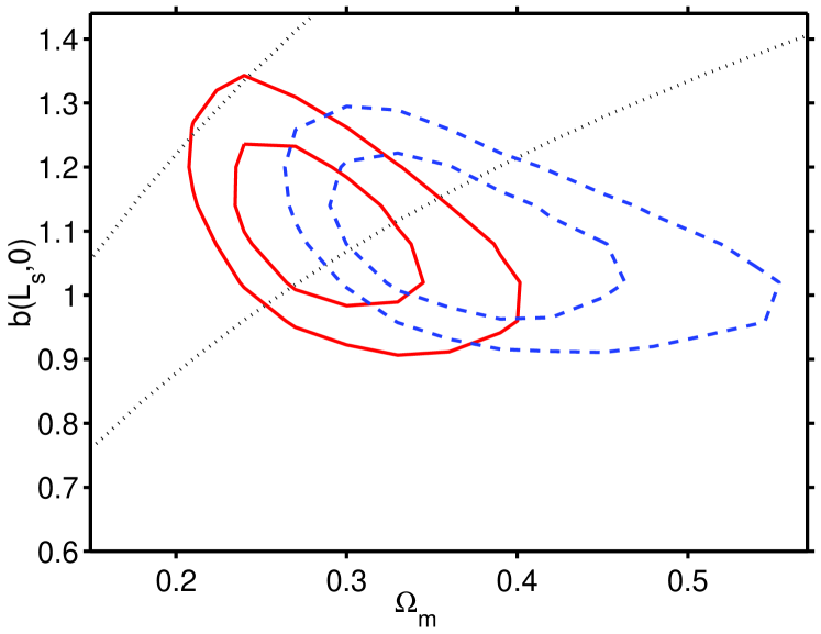
Figure 5: The result of a joint likelihood 2dFGRS+CMB (solid lines). The marginalization (without any external priors) is over $h,\omega_{\rm b}$ and $\sigma_{8{\rm m}}$. Other parameters are held fixed ($n=1,\tau=0$). The contours are for (two-parameter) 68 per cent and 95 per cent confidence intervals. The dotted lines represent the 1-sigma envelope for $\beta(L_{s},0)$, based on $\beta(L_{s},z_{s})=0.43\pm 0.07$ from Peacock et al (2000) and the CGC model. The result of a joint likelihood 2dFGRS+CMB for $n=0.9$ is marked by the dashed contours (68 per cent and 95 per cent).

Table 2: The biasing parameter $b(L_{s},z=0)$ from the full Maximum Likelihood solution (equation 14), and marginalization over ($h,\omega_{\rm b},\sigma_{8{\rm m}},{\Omega_{\rm m}})$ without any external priors (apart from the third entry, where $\omega_{\rm b}=0.02$).

Data	$b(L_{s},0)$
2dFGRS+CBMD ($n=1.0,\tau=0$)	$1.10\pm 0.08$
2dFGRS+CBMD ($n=0.9,\tau=0$)	$1.08\pm 0.09$
2dFGRS+CBMD ($n=1.1,\tau=0$)	$1.15\pm 0.09$
2dFGRS+CBMD ($n=1.0,\tau=0.05,\omega_{\rm b}=0.02$)	$1.06\pm 0.09$

5 Comparison with other measurements

5.1 Other estimates of 2dFGRS amplitude of fluctuations

An independent measurement from 2dFGRS comes from redshift-space distortions on scales $<10{\,h^{-1}\,{\rm Mpc}}$ (Peacock et al. 2000). This gives $\beta(L_{s},z_{s})=0.43\pm 0.07$. In Fig.  5 we show this constraint, after translating it to $\beta(L_{s},z=0)$ via the CGC model. We see consistency with our present analysis at the level of 1-sigma. Using the full likelihood function in the $(b,{\Omega_{\rm m}}$) plane (Fig.  5 ) we derive a slightly larger (but consistent) value, $\beta(L_{s},z_{s})\simeq 0.48\pm 0.06$.

A study of the bispectrum of the 2dFGRS (Verde et al. 2001) on smaller scales ($0.1<k<0.5{\,h\,\rm Mpc^{-1}}$) sets constraints on deviations from linear biasing, and it gives a best-fit solution consistent with linear biasing of unity. The agreement with the result of the present paper is impressive, given that the methods used are entirely different. In fact, by matching the two results one can get constraints on e.g. $\tau\la 0.2$.

5.2 Comparison with other independent measurements

5.2.1 SDSS

Maximum Likelihood analysis of the early Sloan Digital Sky Survey (SDSS) by Szalay et al. (2001) finds from the projected distribution of galaxies in the magnitude bin $20<r^{*}<21$ (median redshift $z_{m}=0.33$) a shape parameter $\Gamma\simeq{\Omega_{\rm m}}h=0.183\pm 0.04$ and a linear real-space $\sigma^{R}_{8{\rm g}}(z=0)=0.785\pm 0.053$ (1-sigma errors), assuming a flat $\Lambda$CDM model with ${\Omega_{\rm m}}=1-{\Omega_{\Lambda}}=0.3$, for the case of no evolution of galaxy clustering, equivalent to our CGC model (see also Dodelson et al. 2001). To convert the SDSS $r^{*}$ magnitude we use models similar to those given in Norberg et al. (2001b), where we find that for $z_{m}\simeq 0.33$, $b_{\rm J}\simeq r^{*}+1$ (for the mix of galaxy populations). Hence at that redshift $r^{*}=20$ corresponds to absolute $M_{b_{\rm J}}\simeq-19.4$ (in a flat ${\Omega_{\rm m}}=0.3$ Universe), which with appropriate $K$ and evolution correction gives a rest-frame $M_{b_{\rm J}}\simeq-19.6$. This is in fact very close to $L_{*}$ of the 2dFGRS. Hence the derived SDSS value, $\sigma^{R}_{8{\rm g}}(L_{*},z=0)=0.785$, is in accord with the real-space values of we get from 2dFGRS.

5.2.2 Cluster abundance

A popular method for constraining $\sigma_{8{\rm m}}$ and ${\Omega_{\rm m}}$ on scales of $\sim 10{\,h^{-1}\,{\rm Mpc}}$ is based on the number density of rich galaxy clusters. Four recent analyses span a wide range of values, but interestingly they are all orthogonal to our CMB and 2dF constraints (Fig. 4) .

Pierpaoli, Scott & White (2001) derived a high value, while Seljak (2001), Reiprich & Boehringer (2002), and Viana, Nichol & Liddle (2002) found lower values:

 

$${\sigma_{8{\rm m}}}$$

  (16)

respectively. For ${\Omega_{\rm m}}=0.3$ these results correspond to $\sigma_{8{\rm m}}\simeq 1.02;0.75;0.68;0.61$ respectively (with typical errors of 10 per cent). The high value agrees with numerous earlier studies by Eke et al. (1998) and others which were based on temperature functions, and it remains to be understood why the recent values are so low. The discrepancy between the different estimates is in part due to differences in the assumed mass-temperature relation. The cluster physics still needs to be better understood before we can conclude which of the above results is more plausible. We see in Fig. 4 that the lower cluster abundance results are actually in good agreement with our value from the 2dFGRS+CMB, $\sigma_{8{\rm m}}\simeq 0.73\pm 0.05$.

5.2.3 Cosmic shear

The measurements of weak gravitational lensing (cosmic shear) are sensitive to the amplitude of the matter power spectrum on mildly non-linear scales. Van Waerbeke et al. (2001), Rhodes, Refregier & Groth (2001) and and Bacon et al. (2002) find respectively

 

$${\sigma_{8{\rm m}}}$$

  (17)

(with errors of about 20 per cent). These estimates are higher than the $\sigma_{8}{\rm m}$ value that we obtain from 2dFGRS+CMB, but note the large error bars in this recently developed method.

6 Discussion

We have combined in this paper the latest 2dFGRS and CMB data. The first main result of this joint analysis is the normalization of the mass fluctuations, $\sigma_{8{\rm m}}=0.73\pm 0.05$. This normalization is lower than the COBE normalization and previous estimates from cluster abundance, but it is actually in agreement with recently revised cluster abundance normalization. The results from cosmic shear are still somewhat higher, but with larger error bars.

The second result is for the biasing parameter for optically-selected $L_{s}$ galaxies, $b(L_{s},0)=1.10\pm 0.08$, which is just consistent with no biasing (‘light traces mass’) on scales of tens of Mpc. When translated to $L_{*}$ via a correction valid for small scales we get a slight anti-bias, $b(L_{*},0)\simeq 0.96$. Although biasing was commonly neglected until the early 1980s, it has become evident that on scales $\la 10{\,h^{-1}\,{\rm Mpc}}$ different galaxy populations exhibit different clustering amplitudes, the so-called morphology-density relation (e.g. Dressler 1980; Hermit et al. 1996; Norberg et al. 2002). Biasing on small scales is also predicted in the simulations of hierarchical clustering from CDM initial conditions (e.g. Benson et al. 2000). It is important therefore to pay attention to the scale on which biasing operates. Our result of linear biasing of unity on scales ($\ga 10{\,h^{-1}\,{\rm Mpc}}$) is actually in agreement with predictions of simulations (e.g. Blanton et al. 2000 Benson et al. 2000; Somerville et al. 2001). It was also demonstrated by Fry (1996) that even if biasing was larger than unity at high redshift, it would converge towards unity at late epochs (see equation 9).

We note that in deriving these results from the 2dFGRS and the CMB, we have had to consider various corrections due to astrophysical and cosmological effects:

• redshift-space distortions cause the amplitude in redshift space to be $\sim 15$ per cent larger than that in real space.

• The evolution of biasing with redshift (for our simple constant galaxy clustering model) gives a biasing that is $\sim 10$ per cent higher at $z_{s}=0.17$ than at redshift zero.

• If luminosity-dependent biasing also holds on large scales then the biasing parameter $b(L_{s}=1.9L_{*})$ is $\sim 15$ per cent higher than that of $L_{*}$ galaxies.

• On the CMB side, an optical depth $\tau=0.05$ due to reionization reduces the derived biasing parameter $b$ by $\sim 5$ per cent. Changing the spectral index from $n=1$ to $n=0.9$ (for both the CMB and 2dFGRS) also reduces $b$ by $\sim 5$ per cent.

While we included these corrections in our analysis we note that they are model dependent, and these theoretical uncertainties combined may account for $\sim 5-10$ per cent uncertainty over and above the statistical random errors.

It may well be that in the future the cosmological parameters will be fixed by CMB, SNe etc. Then, for fixed reasonable cosmological parameters, one can use redshift surveys to study biasing, evolution, etc. This paper is a modest illustration of this approach. Future work along these lines will include exploring non-linear biasing models (e.g. Dekel & Lahav 1999; Sigad, Branchini & Dekel 2001; Verde et al. 2001) per spectral type (Madgwick et al 2002; Norberg et al. 2002; Hawkins et al. (2001, in preparation) and the detailed variation of other galaxy properties with local mass density.

References

- [1] Bacon D.J., Massey R.J., Refregier A.R., Ellis, R.S. 2002, MNRAS, submitted, astro-ph/0203134
- [2] Bahcall N.A., Ostriker J.P., Perlmutter S., Steinhardt P.J., 1999, Science, 284, 148
- [3] Becker R.H., et al., 2001, ApJ, accepted, astro-ph/0108097
- [4] Benson A.J., Cole S., Frenk C.S., Baugh C.M., Lacey C.G., 2000, MNRAS, 311, 793
- [5] Blanton M., Cen R., Ostriker J.P., Strauss M.A., Tegmark M., 2000. ApJ, 531, 1
- [6] Bridle S.L., Eke V.R. Lahav O., Lasenby A.N., Hobson M.P., Cole S., Frenk C.S., Henry J.P., 1999, MNRAS, 310, 565
- [7] Bridle S.L., Zehavi I., Dekel A., Lahav O., Hobson M.P., Lasenby A.N., 2001a, MNRAS, 321, 333
- [8] Bridle S.L., Crittenden R., Melchiorri A., Hobson M.P., Kneissl R., Lasenby A., 2001b, MNRAS, submitted, astro-ph/0112114
- [9] Bunn E.F., White M., 1997, ApJ, 480, 6
- [10] Colless M. & the 2dFGRS team, 2001, MNRAS, 328, 1039
- [11] de Bernardis P., et al., 2002, ApJ, 564, 559
- [12] Dekel A., Lahav O., 1999, ApJ, 520, 24
- [13] Dodelson S. & the SDSS team, 2001, ApJ, submitted, astro-ph/0107421
- [14] Dressler A., 1980, ApJ, 236, 351
- [15] Efstathiou G. & the 2dFGRS team, 2002, MNRAS, 330, 29 (E02)
- [16] Eisenstein D.J., Hu W., 1998, ApJ, 496, 605
- [17] Eke V.R., Cole S., Frank C.S., Henry P.J., 1998, MNRAS, 298, 1145
- [18] Elgaroy O., Gramann M., Lahav O., 2002, MNRAS, 333, 93
- [19] Fan, X., et al., 2002, AJ, 123, 1247
- [20] Feldman H.A., Kaiser N., Peacock J.A., 1994, ApJ, 426, 23
- [21] Freedman W.L., et al., 2001, ApJ, 553, 47
- [22] Fry J.N., 1996, ApJ, 461, L65
- [23] Gawiser E., 2000, Proceedings of PASCOS99 Conference, Lake Tahoe, CA 1999, astro-ph/0005475
- [24] Griffiths, L., Liddle A., 2001, MNRAS, 324, 769
- [25] Halverson N.W., et al., 2002, ApJ, 568, 38
- [26] Hancock S., Rocha G., Lasenby A.N., Gutierrez C.M., 1998, MNRAS, 294, L1
- [27] Hermit S., Santiago B.X., Lahav O., Strauss M.A., Davis M., Dressler A., Huchra J.P., 1996, MNRAS, 283, 709
- [28] Hu W., Eisenstein D.J., Tegmark M., 1998, Phys. Rev. Lett., 80, 5255
- [29] Jaffe A. et al., 2001, Phys. Rev. Lett., 86, 3475
- [30] Kaiser N., 1987, MNRAS, 227, 1
- [31] Kauffmann G., Colberg J.M., Diaferio A., White S.D.M., 1999, MNRAS, 303, 188
- [32] Lahav O., Bridle S.L., Hobson M.P., Lasenby A.L., Sodré L., 2000, MNRAS, 315, 45L
- [33] Lee A.T. et al., 2001, ApJ, 561, L1
- [34] Madgwick D.S. & the 2dFGRS team, MNRAS, 333, 133
- [35] Magliocchetti M., Bagla J., Maddox S.J., Lahav O. 1999, MNRAS, 314, 546
- [36] Matarrese S., Coles P., Lucchin F., Moscardini L., 1997, MNRAS, 286, 95
- [37] Mo H.J., White S.D.M., 1996, MNRAS, 282, 347
- [] Netterfield C.B. et al., 2001, ApJ, accepted, astro-ph/0104460
- [38] Norberg P. & the 2dFGRS team, 2001a, MNRAS, 328, 64
- [39] Norberg P. & the 2dFGRS team, 2001b, MNRAS, submitted, astro-ph/0111011
- [40] Norberg P. & the 2dFGRS team, 2002, MNRAS, 332, 827
- [41] O’Meara J.M. et al., 2001, ApJ, 552, 718
- [42] Peacock J.A. & the 2dFGRS team, 2001, Nature, 410, 169
- [43] Peebles P. J. E. 1980, Large Scale Structure of the Universe, Princeton University Press, Princeton.
- [44] Pen U., 1998, ApJ, 504, 601
- [45] Percival W.J. & the 2dFGRS team, 2001, MNRAS, 327, 1297 (P01)
- [46] Pierpaoli E., Scott D., White M., 2001, MNRAS, 325, 77
- [47] Pryke C. et al., 2002, ApJ, 568, 46
- [48] Reiprich T.H., Boehringer H., 2002, ApJ, 567, 716,
- [49] Rhodes J., Refregier A., Groth E.J., ApJ, submitted, astro-ph/0101213
- [50] Seljak U., 2001, MNRAS, submitted, astro-ph/0111362
- [51] Seljak U., Zaldarriaga M. 1996, ApJ, 469, 437
- [52] Shepherd C.W. et al. 2001, ApJ, 560, 72
- [53] Sigad Y., Branchini E., Dekel A., 1999, ApJ, 520, 24
- [54] Somerville R., Lemson G., Sigad Y., Dekel A., Colberg J., Kauffmann G., White S.D.M., 2001, MNRAS, 320, 289
- [55] Stompor R. et al., 2001, ApJ, 561, L7
- [56] Sutherland W. et al., 1999, MNRAS, 308, 289
- [57] Szalay A.S. & the SDSS team, 2001, ApJ, submitted, astro-ph/0107419
- [58] Tegmark M., Hamilton A.J.S., Xu Y., 2001, astro-ph/0111575
- [59] Van Waerbeke L., et al. 2001, AA, submitted, astro-ph/0101511
- [60] Verde L. et al. & the 2dFGRS team, MNRAS, accepted, astro-ph/0112161
- [61] Viana P.T.P., Nichol R.C., Liddle A.R., 2002, ApJ, 569, L75
- [62] Vittorio N., Silk J., 1991, ApJ, 385, L9
- [63] Wang X., Tegmark M., Zaldarriaga M., 2001, PRD, accepted, astro-ph/0105091 (WTZ)
- [64] Webster M., Bridle S.L., Hobson M.P., Lasenby A.N., Lahav O., Rocha, G., 1998, ApJ Lett, 509, L65
- [65] Zehavi I., et al., 2001, ApJ, accepted, astro-ph/0106476