MODELS OF METAL POOR STARS WITH GRAVITATIONAL SETTLING AND RADIATIVE ACCELERATIONS: I. EVOLUTION AND ABUNDANCE ANOMALIES

Abstract

Evolutionary models have been calculated for Pop II stars of 0.5 to 1.0${\,\mbox{\it M}_{\odot}}$ from the pre-main–sequence to the lower part of the giant branch. Rosseland opacities and radiative accelerations were calculated taking into account the concentration variations of 28 chemical species, including all species contributing to Rosseland opacities in the OPAL tables. The effects of radiative accelerations, thermal diffusion and gravitational settling are included. While models were calculated both for $Z=0.00017$ and $0.0017$, we concentrate on models with $Z=0.00017$ in this paper. These are the first Pop II models calculated taking radiative acceleration into account. It is shown that, at least in a 0.8 $\,\mbox{\it M}_{\odot}$ star, it is a better approximation not to let Fe diffuse than to calculate its gravitational settling without including the effects of $g_{{{\mbox{\scriptsize rad}}}}$(Fe).

In the absence of any turbulence outside of convection zones, the effects of atomic diffusion are large mainly for stars more massive than 0.7${\,\mbox{\it M}_{\odot}}$. Overabundances are expected in some stars with ${{T_{{{\mbox{\scriptsize eff}}}}}}{}\geq 6000$ K. Most chemical species heavier than CNO are affected. At 12 Gyr, overabundance factors may reach 10 in some cases (e.g. for Al or Ni) while others are limited to 3 (e.g. for Fe).

The calculated surface abundances are compared to recent observations of abundances in globular clusters as well as to observations of Li in halo stars. It is shown that, as in the case of Pop I stars, additional turbulence appears to be present.

Series of models with different assumptions about the strength of turbulence were then calculated. One series minimizes the spread on the Li plateau while another was chosen with turbulence similar to that present in AmFm stars of Pop I. Even when turbulence is adjusted to minimize the reduction of Li abundance, there remains a reduction by a factor of at least 1.6 from the original Li abundance. Independent of the degree of turbulence in the outer regions, gravitational settling of He in the central region reduces the lifetime of Pop II stars by 4 to 7 % depending on the criterion used. The effect on the age of the oldest clusters is discussed in an accompanying paper.

Just as in Pop I stars where only a fraction of stars, such as AmFm stars, have abundance anomalies, one should look for the possibility of abundance anomalies of metals in some Pop II turnoff stars, and not necessarily in all. Expected abundance anomalies are calculated for 28 species and compared to observations of M92 as well as to Li observations in halo field stars.

1 Astrophysical context

Helioseismology has confirmed the importance of gravitational settling in the Sun’s external regions (Guzik & Cox 1992; Guzik & Cox 1993; Christensen-Dalsgaard et al. 1993; Proffitt 1994; Bahcall et al. 1995; Guenther et al. 1996; Richard et al. 1996; Brun et al. 1999). Turnoff stars in globular clusters are only slightly less massive than the Sun and have convection zones that tend to be somewhat shallower. In solar type stars, radiative accelerations have been shown to become equal to gravity for some metals around the end of the main sequence lives (Turcotte et al., 1998b). The question of the atomic diffusion of metals in Pop II stars then naturally arises. It is currently of special interest because large telescopes are now making possible the determination of the abundance of metals in the turnoff stars of globular clusters. In this paper evolutionary models that take into account the diffusion of He, LiBeB and metals in Pop II stars are presented for the first time. Surface abundances may then be used as additional constraints in the determination of the age of globular clusters and of the Universe (VandenBerg et al. 2001, hereafter Paper II). Given their old age, Pop II stars are those where the slow effect of atomic diffusion has the largest chance to play a role on the evolutionary properties. Previously published evolutionary models of Pop II stars have included some of the effects of diffusion (Deliyannis et al. 1990; Proffitt & Michaud 1991a; Proffitt & VandenBerg 1991; Salaris et al. 2000; Stringfellow et al. 1983) but never included the effects of the diffusion of metals with their radiative accelerations self consistently.

Determining constraints on stellar hydrodynamics from abundance observations requires knowing the original chemical composition of the star. In Pop II stars there are larger variations in original abundances than in Pop I. For that reason it is essential to use globular clusters for abundance determinations of metals since only then does one have a handle on the original abundances from observations of cluster giants. However LiBeB have an origin partly different from that of most metals. Coupled with their sensitivity to low temperature nuclear burning, their abundance determination in halo stars provides useful constraints on hydrodynamics even if determinations in cluster stars would be preferable.

The observation by Spite & Spite (1982) of a plateau in the Li concentration over a relatively large $T_{{{\mbox{\scriptsize eff}}}}$ interval of Pop II stars has now been confirmed by many observations. Furthermore, the Li concentration is constant while that of Fe varies by more than a factor of 100 (Cayrel, 1998) from $[\mbox{Fe}/\mbox{H}]=-3.7$ to $-1.5$. This shows the primordial origin of Li. Its preservation for such a time interval over such a wide $T_{{{\mbox{\scriptsize eff}}}}$ interval seriously challenges our understanding of convection and other potential mixing processes in those stars (Michaud et al., 1984). If there were no mixing process outside of convection zones, the surface Li abundance would vary with $T_{{{\mbox{\scriptsize eff}}}}$: at small $T_{{{\mbox{\scriptsize eff}}}}$ because of nuclear reactions (${}^{7}\mbox{Li}(p,\alpha)^{4}\mbox{He}$) and at large $T_{{{\mbox{\scriptsize eff}}}}$ because of gravitational settling. Extending convection zones by a simple turbulence model does not solve the problem since, if the extension is sufficient to reduce Li settling enough in the hotter stars, it causes excessive Li destruction in the cooler stars of the plateau (Proffitt & Michaud, 1991a). Efforts were also made to link such an extension to differential rotation (Vauclair 1988 or, as parametrized in the Yale models, Pinsonneault et al. 1999) but the small apparent dispersion in the plateau makes this model unlikely. Ryan et al. (1999) even claim that the destruction may not be by more than 0.1 dex.

Several groups (Cayrel et al. 1999, Hobbs & Thorburn 1994, 1997, Smith et al. 1993) have also observed ${}^{6}\mbox{Li}$ in halo stars. Since ${}^{6}\mbox{Li}$ is destroyed at a smaller $T_{{{\mbox{\scriptsize eff}}}}$ than ${}^{7}\mbox{Li}$, its survival in old stars implies a strict and small upper limit on the amount of mixing in those stars. The stars where a detection has been made are all concentrated close to the turnoff (Cayrel et al., 1999). While a mechanism has been suggested to produce ${}^{6}\mbox{Li}{}$ in the Sun (Ramaty et al., 2000), it is not expected to significantly affect atmospheric values so that a star in which ${}^{6}\mbox{Li}{}$ is seen in the atmosphere may not have destroyed a significant fraction of its original ${}^{6}\mbox{Li}$.

Boesgaard et al. (1999) determined Be abundances in halo stars as well as a linear correlation with the Fe abundance suggesting that Be has not been destroyed in those stars.

The chemical composition of globular clusters is attracting more attention as large telescopes make the determination of the surface chemical composition of turnoff stars possible. The determination of the abundance of metals makes it possible to put additional constraints on the hydrodynamics of Pop II stars. Some observers have reported factors of 2 differences between Fe abundances in red giants and subgiants (King et al., 1998). However Ramirez et al. (2001) and Gratton et al. (2001) find no difference between the Fe abundances in red giants and turnoff stars. Thévenin et al. (2001) find the same relative abundances as in the Sun in the turnoff stars of NGC 6397. Unexplained anticorrelations between the abundances of O and Na have been observed by Gratton et al. (2001).

In this paper, the surface abundances to be expected in Pop II stars are calculated under different assumptions for the internal stellar hydrodynamics. The first and simplest assumption is that there is no macroscopic motion outside of convection zones. There remains only atomic diffusion, including the effects of gravitational settling, thermal diffusion and radiative accelerations, as a transport process outside of convection zones. On the main sequence, such models have been shown to lead to larger abundance anomalies than are observed (Turcotte et al., 1998a) but also to the appearance of an additional convection zone caused by the accumulation of iron peak elements (Richard et al., 2001). A relatively simple parametrization of turbulence, corresponding to an extension of those Fe convection zones by a factor of about 5 in mass, was shown to lead to a simple explanation of the AmFm phenomenon (Richer et al., 2000). A similar parametrization is used here in Pop II stars and leads to our second series of models. Finally, we use an additional parametrization that is chosen in order to minimize the reduction of the surface Li concentration, so as to provide the best representation of the Spite plateau. Proffitt & Michaud (1991a) introduced a similar parametrization of turbulence to compete with He and Li settling (other parametrizations of turbulence were introduced for the Sun by Richard et al. 1996 and Brun et al. 1999). Basu (1997) has shown that weak turbulence below the solar convection zone also improves agreement with the solar pulsation spectrum. For comparison purposes, series of models are also calculated without diffusion and one model is calculated with gravitational settling but without $g_{{{\mbox{\scriptsize rad}}}}$ (see subsubsection 3.2.2).

2 CALCULATIONS

2.1 Models

The models were calculated as described in Turcotte et al. (1998b). The radiative accelerations are from Richer et al. (1998) with the correction for redistribution from Gonzalez et al. (1995) and LeBlanc et al. (2000). The atomic diffusion coefficients were taken from Paquette et al. (1986). The uncertainties in the atomic and thermal diffusion coefficients have been discussed by Michaud & Proffitt (1993), and by Michaud (1991) in particular for the temperature–density domain of the interior of Pop II stars and the Sun.

Turbulent transport is included as in Richer et al. (2000) and Richard et al. (2001) where the parameters specifying turbulent transport coefficients are indicated in the name assigned to the model. For instance, in the T5.5D400-3 model, the turbulent diffusion coefficient, $D_{\rm{T}}$, is 400 times larger than the He atomic diffusion coefficient at $\log T=5.5$ and varying as $\rho^{-3}$. To simplify writing, T5.5 will also be used instead of T5.5D400-3 since all models discussed in this paper have the D400-3 parametrization. The $\rho^{-3}$ dependence is suggested (see Proffitt & Michaud 1991b) by observations that the Be solar abundance today is hardly smaller than the original Be abundance (see for instance Bell et al. 2001)

All models considered here were assumed to be chemically homogeneous on the pre-main sequence with the abundance mix appropriate for Pop II stars. The relative concentrations used are defined in Table 1. The relative concentrations of the alpha elements are increased compared to the solar mix as is believed to be appropriate in Pop II stars (VandenBerg et al., 2000).

2.2 Mixing length

In Turcotte et al. (1998b), the solar luminosity and radius at the solar age were used to determine the value of $\alpha{}$, the ratio of the mixing length to pressure scale height, and of the He concentration in the zero age Sun. They calibrated $\alpha{}$ both in models using Krishna-Swamy’s $T(\tau){}$ relation (Krishna Swamy, 1966) (both with and without atomic diffusion) and in models using Eddington’s $T(\tau){}$ relation (only with diffusion). The He concentration mainly affects the luminosity while $\alpha{}$ mainly determines the radius, through the depth of the surface convection zone. The required value of $\alpha{}$ was found to be slightly larger in the diffusive than in the non diffusive models because an increased value of $\alpha{}$ is needed to compensate for He and metals settling from the surface convection zone. The increased $\alpha{}$ in the diffusion models of the Sun is then determined by the settling occurring immediately below the solar surface convection zone. See Freytag & Salaris (1999) for a discussion of uncertainties related with the use of the mixing length in Pop II stars.

Some of the models presented in this paper were calculated with turbulence below the convection zone. The appropriate value of $\alpha{}$ to use then depends on the depth of turbulence. If turbulence is large enough to eliminate settling at the depth of solar models, the most appropriate $\alpha{}$ to use is that determined for non diffusing solar models. If the adopted turbulence is more superficial than the solar convection zone, the appropriate $\alpha{}$ to use is that for the solar models with diffusion. Given the uncertainty, it was chosen to use the same value of $\alpha$ for all models, both with and without diffusion, calculated with Eddington’s $T(\tau){}$ relation. In order to give an estimate of the uncertainty related to $\alpha{}$, two values of $\alpha{}$ (one determined by the solar model without diffusion and one by the solar model with diffusion) will be used for one series of models with diffusion (see subsection 3.3).

The calculated series of models are identified in Table 2. The series labeled KS$\alpha{}$ used a value of $\alpha{}$ determined from a solar model with diffusion while the series labeled KS used a value of $\alpha{}$ determined from a solar model without diffusion.

3 EVOLUTIONARY MODELS

Four series of evolutionary models were calculated. In the first subsection, the models with atomic diffusion are presented. In the second one, the models with turbulence and those without diffusion are introduced and compared to the models with atomic diffusion. Two series of models with turbulence are discussed in some detail: a series that minimizes Li underabundance and one that contains a level of turbulence similar to that needed to reproduce the observations of AmFm stars. In the last subsection, the effect of changing boundary conditions is analyzed.

3.1 Evolution with atomic diffusion

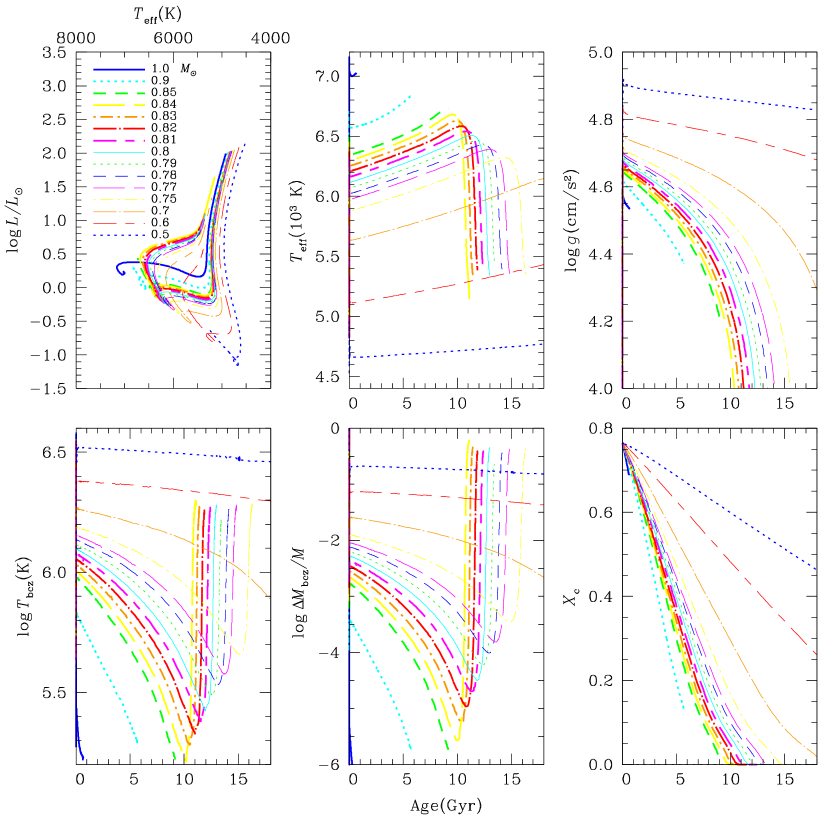
Figure 1: Hertzsprung-Russell diagram, and time evolution of $T_{{{\mbox{\scriptsize eff}}}}$, $\log g$, temperature at the base of the surface convection zone ($T_{{{\mbox{\scriptsize bcz}}}}$), mass above the base of the surface convection zone $M_{{{\mbox{\scriptsize bcz}}}}$ and mass fraction of hydrogen ($X_{c}$) at the center of stars of 0.5 to 1.0 $\,\mbox{\it M}_{\odot}$ with $Z$ = 0.00017, or $[\mbox{Fe}/\mbox{H}]=-2.31.$ All models were calculated with atomic diffusion and radiative accelerations but no turbulent transport. In the black and white figure, are shown 6 of the 15 models that may be seen in the color figure available in the electronic version of the paper.

The $T_{{{\mbox{\scriptsize eff}}}}$ and $\log{}g$ as a function of age as well as the luminosity as a function of $T_{{{\mbox{\scriptsize eff}}}}$ are shown in Figure 1 for evolutionary models calculated including atomic diffusion and only those physical processes that can currently be evaluated properly from first principles. That figure also contains the time variation of the depth of the surface convection zone, of the temperature at its bottom and of central H concentration. Models were calculated for 0.5 to 1.0 $\,\mbox{\it M}_{\odot}$ stars from the pre-main–sequence to the bottom of the giant branch except for the 0.85, 0.9 and 1.0 $\,\mbox{\it M}_{\odot}$ stars which were stopped earlier because of numerical instabilities. All models shown have $Z=0.00017$. The mass interval was chosen to minimize the possibility of interpolation errors in the construction of isochrones (see Paper II).

The variation of the mass in the surface convection zone is large enough to play a major role on surface abundance evolution. In the next two subsections, the effect of radiative accelerations on surface abundances are related to the regression of the surface convection zone during evolution.

3.1.1 Radiative accelerations

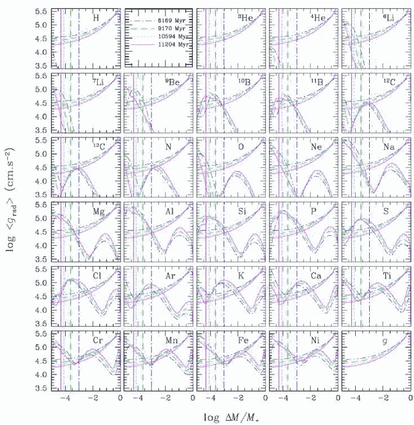
Figure 2: Radiative accelerations in a Pop II star of 0.8 $\,\mbox{\it M}_{\odot}$ with $[\mbox{Fe}/\mbox{H}]=-2.31$ at four epochs identified in the upper part of the figure. The vertical lines give the position of the bottom of the surface convection zone. For other stellar masses, it is the position of the bottom of the convection zone that is most different. The $g_{{{\mbox{\scriptsize rad}}}}$ of the various species varies from star to star but much less than the depth of convection zones. Gravity is shown in the lower right hand corner and repeated in each panel of the figure.

The radiative accelerations below the surface convection zone play the most important role in determining the surface abundance variations (see Fig. 2). As the evolution of a 0.8 $\,\mbox{\it M}_{\odot}$ star proceeds during the main sequence phase, the surface convection zone becomes progressively thinner: between 6 and 11 Gyr, the mass in the convection zone is reduced by a factor of about 20, from $\log\Delta M/{\it\,M_{*}}=-3.0$ to $-4.3$ (see Fig. 1). The effect of this regression of the surface convection zone may be seen in the surface abundances through the dependence of $g_{{{\mbox{\scriptsize rad}}}}$ on nuclear charge. The $g_{{{\mbox{\scriptsize rad}}}}$ on Li has a maximum at $\log\Delta M/{\it\,M_{*}}\simeq-5$ where it is in the hydrogenic configuration. It is completely ionized deeper in the star so that $g_{{{\mbox{\scriptsize rad}}}}$(Li) is progressively reduced deeper in. The chemical species with a larger nuclear charge become ionized deeper in so that they are in an hydrogenic configuration deeper in and have the related maximum of their $g_{{{\mbox{\scriptsize rad}}}}$ at greater depths. For B, it is at $\log\Delta M/{\it\,M_{*}}\simeq-4$, for O at $\log\Delta M/{\it\,M_{*}}\simeq-2$ and for Si at $\log\Delta M/{\it\,M_{*}}\simeq-1$. Another maximum in the $g_{{{\mbox{\scriptsize rad}}}}$ appears when a species is in between the atomic configurations of Li and F. This maximum occurs at $\log\Delta M/{\it\,M_{*}}\simeq-4$ for P, and $-2$ for Cr. These maxima may be followed on the figure for other species. As may be seen from Figure 2, when the atomic species is in the hydrogenic configuration, the $g_{{{\mbox{\scriptsize rad}}}}$ is rarely larger than gravity. It is larger only for Be, B and C. At the maximum of $g_{{{\mbox{\scriptsize rad}}}}$ between the Li-like and F-like configurations, however, $g_{{{\mbox{\scriptsize rad}}}}$ is usually larger than gravity. Contrary to what happens in Pop I stars (Richer et al., 1998), the $g_{{{\mbox{\scriptsize rad}}}}$ do not depend on the abundance of the species since it is too small to cause flux saturation.

3.1.2 Abundances

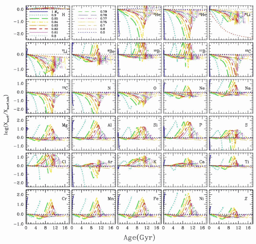
Figure 3: Surface abundance variations in Pop II stars of 0.5 to 1.0 $\,\mbox{\it M}_{\odot}$ with $[\mbox{Fe}/\mbox{H}]=-2.31$. All models were calculated with atomic diffusion and radiative accelerations but no turbulent transport. In the black and white figure, are shown 6 of the 15 models that may be seen in the color figure available in the electronic version of the paper. As is evident in the color version, a vertical line drawn in each panel of the figure, corresponding to a fixed age, permits one to evaluate the range of surface abundances of a species at that age (in, e. g., a globular cluster).

The time variation of surface abundances in Pop II stars with atomic diffusion is shown in Figure 3. The surface abundances reflect the variation of the $g_{{{\mbox{\scriptsize rad}}}}$ below the surface convection zone as it moves toward the surface. From Figure 1, one sees that the depth of the surface convection zone gets progressively smaller during evolution until hydrogen is exhausted from the center. In the 0.8 $\,\mbox{\it M}_{\odot}$ model, it starts at a depth of $\log\Delta M/{\it\,M_{*}}\simeq-2$ and is at $\log\Delta M/{\it\,M_{*}}\simeq-4.5$ after 11 Gyr. One sees in Figure 2 that $g_{{{\mbox{\scriptsize rad}}}}$(Fe) is smaller than gravity when the convection zone is deep but larger than gravity when it is more superficial. In the early evolution, Fe settles gravitationally though less rapidly than He or C, largely because $g_{{{\mbox{\scriptsize rad}}}}$(Fe) is not much smaller than gravity. Around 9 Gyr, $g_{{{\mbox{\scriptsize rad}}}}$(Fe) becomes larger than gravity below the surface convection zone. One sees the effect in the surface abundances (Figure 3) where the surface Fe concentration starts increasing around 9 Gyr, becoming larger than the original concentration around 10 Gyr and reaching an overabundance by a factor of about 5 just before the star becomes a subgiant, at which point the Fe abundance goes back to very nearly its original value as the convection zone becomes more massive. Similar remarks apply to other chemical species.

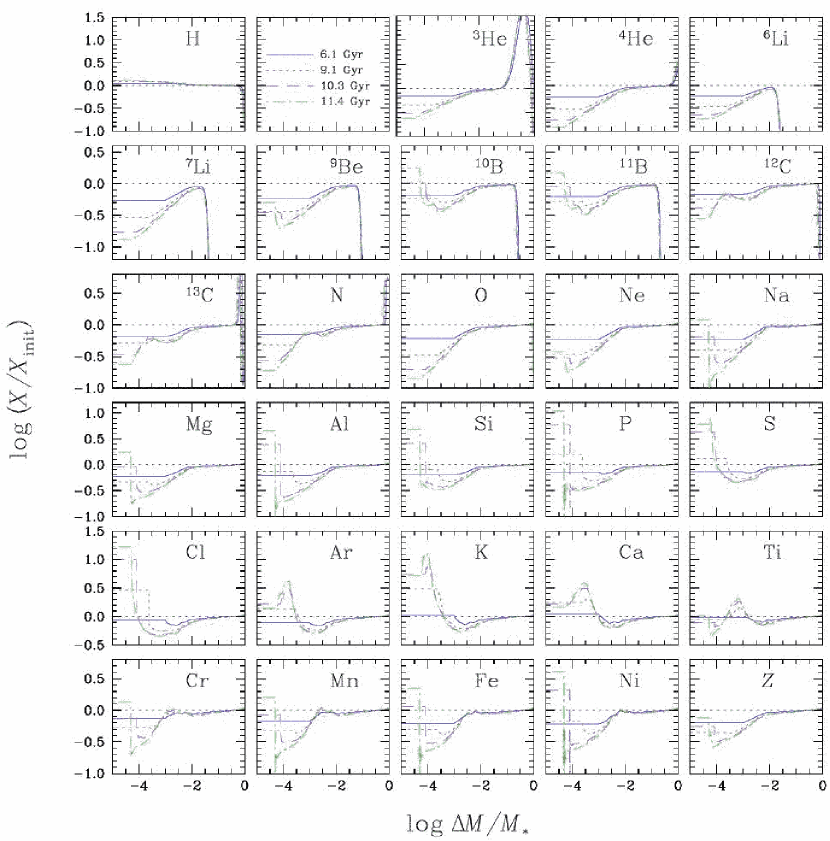
Figure 4: Internal abundance variations in a Pop II star of 0.8 $\,\mbox{\it M}_{\odot}$ with $[\mbox{Fe}/\mbox{H}]=-2.31$. The profiles are shown at four different ages, 6.1, 9.1, 10.3 and 11.4 Gyr. The last is shortly before the star moves to the giant branch. Calculations included atomic diffusion and radiative accelerations but no turbulent transport.

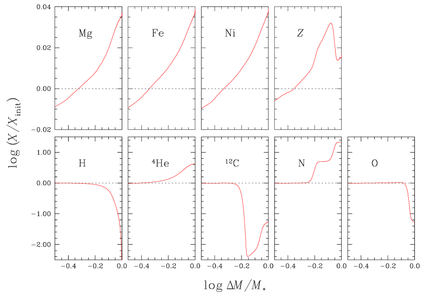
Figure 5: Abundance variations in a Pop II star of 0.8 $\,\mbox{\it M}_{\odot}$ with $[\mbox{Fe}/\mbox{H}]=-2.31$ over the inner 2/3 of the mass of the star at an age of 11.8 Gyr. Calculations included atomic diffusion and radiative accelerations but no turbulent transport. The zero abundance change occurs around 1/2 the mass of the star at $\log\Delta M/{\it\,M_{*}}\simeq-0.3$. Interior to that point, the abundance of metals is generally larger than the original abundance. The variations of CNO are due to their transformation by the CNO chain which would lead to a decrease of Z at the center if it were not for the settling of the other metals. Only Mg, Fe and Ni are shown from the 16 species between Ne and Ni included in the calculations but all others have very similar behavior.

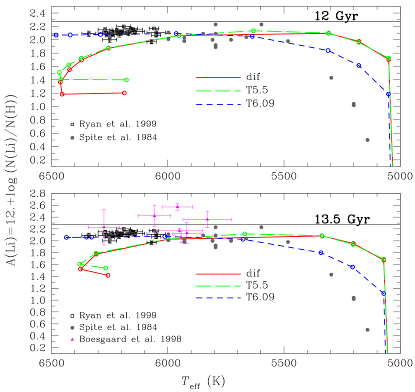
Figure 15: Lithium surface abundances after 12 and 13.5 Gyr of evolution for 3 turbulence strengths: no turbulence, similar to AmFm stars (T5.5) and minimizing Li surface abundance variations (T6.09). Segmented straight lines link calculated values. In comparing results for different turbulence models for ${{T_{{{\mbox{\scriptsize eff}}}}}}\leq$ 6000 K, one should remember that, at a given mass and age, a star with the T6.09 turbulence model has a higher $T_{{{\mbox{\scriptsize eff}}}}$ (by some 100  K) than one with atomic diffusion only (see Fig. 7). References for the observed Li abundances are identified on the figure.

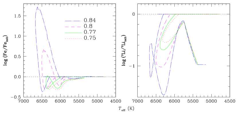
Figure 16: Lithium and Fe surface abundances as a function of $T_{{{\mbox{\scriptsize eff}}}}$ throughout the main sequence and subgiant evolution of 0.84, 0.8, 0.77 and 0.75 $\,\mbox{\it M}_{\odot}$ stars when atomic diffusion is included in the calculations. Turbulence is assumed negligible. For the 0.84 $\,\mbox{\it M}_{\odot}$ star the main sequence starts at $T=6300$K where $\mbox{Fe}=\mbox{Fe}_{0}$. As evolution proceeds, the Fe abundance decreases until an underabundance of $-$0.4 dex is reached. At that point, the surface convection zone has retracted sufficiently for $g_{{{\mbox{\scriptsize rad}}}}$(Fe) to be greater than gravity and the Fe abundance increases up to a 1.7 dex overabundance. This occurs at the end of the main sequence evolution (around the turnoff) at ${{T_{{{\mbox{\scriptsize eff}}}}}}=6600$K. As evolution proceeds on the subgiant branch the surface convection zone gets deeper and the Fe abundance decreases to 0.1 dex below the original abundance. The Fe abundance goes back to its original value when a $T_{{{\mbox{\scriptsize eff}}}}$ of 5300$-$5400 K is reached. Similar evolution occurs for the other stars except that it starts at different $T_{{{\mbox{\scriptsize eff}}}}$ for each. The Li abundance in the 0.84 $\,\mbox{\it M}_{\odot}$ star has a similar evolution. The Li abundance decreases until an underabundance of $-$1.2 dex is reached. At that point, the surface convection zone has retracted sufficiently for $g_{{{\mbox{\scriptsize rad}}}}$(Li) to be greater than gravity. However $g_{{{\mbox{\scriptsize rad}}}}$(Li) is larger than gravity over a smaller interval than $g_{{{\mbox{\scriptsize rad}}}}$(Fe). It leads to an increase of the Li abundance at ${{T_{{{\mbox{\scriptsize eff}}}}}}=6700$K but to no overabundance. As the subgiant evolution starts, Li gets below its main sequence abundance at ${{T_{{{\mbox{\scriptsize eff}}}}}}=6500$K, creating a loop in the Li abundance curve. The Li abundance never reaches its original abundance since, before this occurs, the surface convection zone approaches the region of Li burning and the Li abundance decreases rapidly below 5800 K .

The depth dependence of the abundance variations is shown for a 0.8 $\,\mbox{\it M}_{\odot}$ model in Figure 4. One first notices that the abundance of ${}^{6}\mbox{Li}$ is modified by nuclear reactions over the inner 98 % of the mass. Atomic diffusion modifies the abundances over the outer 1 % of the mass. This leaves hardly any intermediate zone. At 6.1 Gyr, the surface convection zone extends down to $\log\Delta M/{\it\,M_{*}}\simeq-3.0$, where the $g_{{{\mbox{\scriptsize rad}}}}$ are smaller than gravity for most species. Only K, Ca and Ti start to be supported: their abundances in the surface convection zone are larger than immediately below. As evolution proceeds, the convection zone recedes. After 9.1 Gyr, atomic species between Na and Ni are supported as the $g_{{{\mbox{\scriptsize rad}}}}$ is larger than gravity below the bottom of the convection zone. This continues as the evolution proceeds. After 11.4 Gyr, the Fe abundance, for instance, is 3 times larger than the original abundance in the surface convection zone. That increased concentration of Fe is caused by the migration of Fe above $\log\Delta M/{\it\,M_{*}}\simeq-3.5$ where its $g_{{{\mbox{\scriptsize rad}}}}$ becomes larger than gravity. Between $\log\Delta M/{\it\,M_{*}}\simeq-4.5$ and $-2$, the concentration of Fe decreases since it is either pushed into the surface convection zone by radiative accelerations (for $\log\Delta M/{\it\,M_{*}}\geq-3.5$) or settles gravitationally below. On the scale of that figure, the concentration variations of Fe are not seen for $\log\Delta M/{\it\,M_{*}}\geq-2$. It sinks toward the center of the star where a small Fe overabundance appears. The diffusion time scales are long enough that the effects amount to nearly a 10 % increase at the center after 11.4 Gyr (see Fig. 5). This figure may be compared to Figures 15 and 16 of Turcotte et al. (1998b) where the increase in Fe concentration at the center is by about 3 % at the age of the Sun. Transformation of C and O into N also modifies the value of $Z$ so that it increases by only 4 % at the center and has a maximum outside of the region where O is transformed into N.

In stars of other masses, surface abundances are also mainly determined by the depth reached by the surface convection zone. In the 0.7 $\,\mbox{\it M}_{\odot}$ model, the surface convection zone never gets thinner than $\log\Delta M/{\it\,M_{*}}\simeq-3$ so that no overabundances appear during evolution and underabundances are limited to a factor of about 2. In the 0.9$\,\mbox{\it M}_{\odot}$ model on the other hand, the surface Fe abundance starts increasing around 2 Gyr, when the surface convection zone becomes thinner than $\log\Delta M/{\it\,M_{*}}\simeq-4$, where, as seen above, $g_{{{\mbox{\scriptsize rad}}}}$(Fe) becomes larger than gravity. In this star, Fe becomes overabundant around 3 Gyr. In Pop II stars of larger mass, the overabundances are larger because the surface convection zones are thinner.

3.2 Evolution with turbulent diffusion

3.2.1 Turbulent diffusion coefficient and Li abundance

From Figure 1, one sees that even in one single model, say the 0.8 $\,\mbox{\it M}_{\odot}$ one, the mass in the convection zone varies from about $\log\Delta M/{\it\,M_{*}}\simeq-2.1$ to $-4.2$ during the main–sequence evolution. Linking turbulence to the position of the convection zone could never produce a small variation of Li: if one increased the depth of the convection zone by a fixed factor, large enough to eliminate settling around 11 Gyr for instance (a factor of 100 or so is needed), this would lead to complete destruction of Li in the early evolution. To minimize Li abundance reduction, it is essential, if one uses time independent parametrization, to link turbulence to a fixed $T$ and not to the bottom of convection zones.

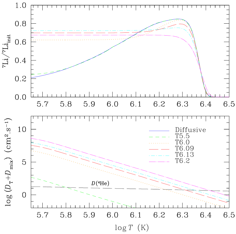
Figure 6: Temperature dependence of atomic and turbulent diffusion coefficients in 0.8 $\,\mbox{\it M}_{\odot}$ models. The nearly horizontal line is the He atomic diffusion coefficient. The other lines are various parametrizations of turbulence. In the upper part of the figure, the corresponding Li concentrations are shown, at an age of 10.2 Gyr, with the same line identification to give the link between turbulent transport and Li burning at $\log T\simeq 6.4$. The parameters specifying turbulent transport coefficients are indicated in the name assigned to the model. For instance, in the T5.5D400-3 model, the turbulent diffusion coefficient, $D_{\rm{T}}$, is 400 times larger than the He atomic diffusion coefficient at $\log T=5.5$ and varying as $\rho^{-3}$.

The turbulent transport coefficients used in these calculations are shown in Figure 6. We chose to introduce the turbulence that minimizes the reduction of the surface Li abundance. We consequently defined the turbulent diffusion coefficient as a function of $T$ in order to adjust it most closely to the profile that limits gravitational settling of Li while not burning Li. The nuclear reaction ${}^{7}\mbox{Li}(p,\alpha)^{4}\mbox{He}$ is highly $T$ sensitive and the Li burning occurs at $\log T\simeq 6.4$ (see Lumer et al. 1990 for a detailed discussion). Turbulent diffusion was adjusted to be smaller than atomic diffusion slightly below that $T$ so that turbulence would reduce settling as much as is possible in surface layers without forcing Li to diffuse by turbulence to $\log T\simeq 6.4$.

A few series of evolutionary models were run in order to optimize turbulence parameters. Examples of the resultant interior Li profiles are shown in Figure 6. The Li concentration always goes down rapidly as a function of increasing $T$ for $\log T\simeq 6.4$. In the absence of turbulence, there is a peak in the Li concentration at $\log T\simeq 6.3$. This peak disappears as the strength of turbulence is increased. Turbulence in the T5.5D400-3 model is too weak to influence Li concentration in the $T$ interval shown. Turbulence in the T6.0D400-3 model eliminates the Li abundance gradient caused by gravitational settling down to $\log T\simeq 6.1$ while causing little reduction on the largest Li abundance at $\log T\simeq 6.3$. Increasing turbulence further reduces the Li peak, and in the T6.2 model the surface Li abundance is smaller than in the T6.13 model, showing that one has passed the optimal value of turbulence.

It is interesting to note that the turbulent diffusion coefficient of the T6.09D400-3 model of 0.8 $\,\mbox{\it M}_{\odot}$ is a factor of about 10 smaller than the turbulent diffusion coefficient found necessary to reproduce the solar Li surface abundance by Proffitt & Michaud (1991b). The latter corresponds approximately to the T6.2D400-3 turbulent diffusion coefficient profile. On the other hand the T5.5D400-3 turbulent diffusion parametrization corresponds approximately, as a function of $T$, to that found by Richer et al. (2000) to lead to the abundance anomalies observed in AmFm stars.

3.2.2 Diffusion and stellar structure

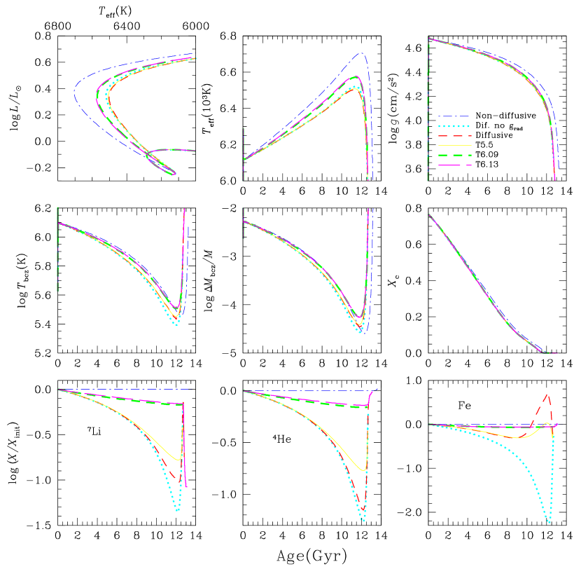
Figure 7: Hertzsprung-Russell diagram, and time evolution of $T_{{{\mbox{\scriptsize eff}}}}$, $\log g$, temperature at the base of the surface convection zone ($T_{{{\mbox{\scriptsize bcz}}}}$), mass at the base of the surface convection zone ($M_{{{\mbox{\scriptsize bcz}}}}$) and mass fraction of hydrogen ($X_{c}$) at the center and of the He, Fe and Li abundances in 0.8 $\,\mbox{\it M}_{\odot}$ models both with and without diffusion. See Figure 6 and Table 2 for a definition of the notation used for models with turbulent transport.

A comparison of the 0.8 $\,\mbox{\it M}_{\odot}$ models with and without diffusion is shown in Figure 7. First compare the Hertzsprung-Russell diagrams. All models with diffusion (both with and without turbulence) nearly have the same evolutionary tracks (those with turbulence are somewhat hotter). However the one without atomic diffusion goes to significantly higher $T_{{{\mbox{\scriptsize eff}}}}$ than all models with diffusion. We have also verified that the turnoff temperature is reached 6 to 7 % earlier in the models with diffusion (with or without turbulence) than in the model without diffusion. These differences are reflected in the isochrones based on these tracks and therefore on globular cluster age determinations (see Paper II). They partially come from the structural effects of the global redistribution of He but also from the 4 to 5 % difference in the age at which the central H abundance is exhausted. This in turn is reflected in the shorter age (also 4 to 5 %) at which all diffusion models become subgiants, as seen in the rapid decrease of $T_{{{\mbox{\scriptsize eff}}}}$ but the rapid increases of the mass and $T$ at the bottom of the surface convection zone.

While there are significant differences between the model without diffusion and all those with diffusion, the effect of the different turbulent transport models on the depth and mass at the bottom of the surface convection zone, and the time variation of the central H concentration are seen from Figure 7 to be practically negligible on the scale of that figure. Of the macroscopic properties defining the evolution of a 0.8$\,\mbox{\it M}_{\odot}$ star, only the $T_{{{\mbox{\scriptsize eff}}}}$ and $\log g$ appear to be modified by the turbulence models that were introduced. While it is not shown for other masses, it is also true for them. However it is shown in Paper II that the differences in $T_{{{\mbox{\scriptsize eff}}}}$ that seem small on the scale of Figure 7 are important in the comparison of calculated and observed isochrones.

Given that there are, in the literature, calculations of Pop II evolutionary tracks with gravitational settling but no $g_{{{\mbox{\scriptsize rad}}}}$, it is worth noting that the track ($L-{{T_{{{\mbox{\scriptsize eff}}}}}}{}$ relation; upper left hand part of Fig. 7) of such a model is, around turnoff, slightly cooler than the track of the model with diffusion and $g_{{{\mbox{\scriptsize rad}}}}$ but no turbulence. Furthermore the Fe abundance is very different, by a factor of about 1000, at 12 Gyr. The $T_{{{\mbox{\scriptsize bcz}}}}$ is smaller by 0.1 dex mainly because of the reduction of opacity caused by the reduction of the Fe abundance. It is a better approximation not to let Fe diffuse at all in a 0.8$\,\mbox{\it M}_{\odot}$ star than to calculate its gravitational settling without including the effects of $g_{{{\mbox{\scriptsize rad}}}}$(Fe). The Li abundance is smaller by a factor of 2 in this case both because of the reduction of the $T_{{{\mbox{\scriptsize bcz}}}}$ and because $g_{{{\mbox{\scriptsize rad}}}}$(Li) has some effect in the 0.8 $\,\mbox{\it M}_{\odot}$ model.

3.2.3 Stellar structure and abundances

The surface abundance anomalies caused by atomic diffusion are much more affected by turbulence than the macroscopic properties. In the T5.5 model, turbulence reduces surface abundance anomalies but only in the time interval from 9 to 12 Gyr. Before 9 Gyr, the surface convection zone is deeper than $\log T\simeq 5.7$ while in the T5.5D400-3 model, the turbulent diffusion coefficient is larger than atomic diffusion only for temperatures up to $\log T\simeq 5.8$. Only when the surface convection zone has retracted sufficiently for turbulent diffusion to be larger than atomic diffusion below the convection zone, does turbulence have any effect. In this model, the turbulent diffusion coefficient does not suppress completely the effects of atomic diffusion (see Fig. 7). It reduces them by an amount dependent on the chemical species. An Fe overabundance appears in the absence of turbulence but it is eliminated in the T5.5 model while the He underabundance is much less affected. The T6.0 model has the same turbulence profile as the T5.5D400-3 model except that the profile is shifted towards higher temperatures by a factor of 3 in $T$ (see Fig. 6); this leads to a much larger effect on abundance anomalies. It limits the effect of atomic diffusion on the surface abundances of He and Li to a factor of $\simeq{}1.6$.

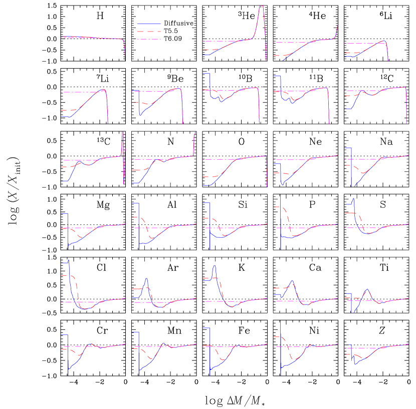
Figure 8: Internal abundance profiles in a Pop II star of 0.8 $\,\mbox{\it M}_{\odot}$ with $[\mbox{Fe}/\mbox{H}]=-2.31$ and turbulence parametrized by T6.09D400-3 and T5.5D400-3. The model with no turbulence is also shown for comparison purposes. The profiles are shown at 11.7 Gyr, shortly before the star moves to the giant branch. The same scale is used as for Figure 4. See Figure 6 and Table 2 for a definition of the notation used for models with turbulent transport.

The effect of turbulent transport on the interior concentrations in a 0.8 ${\,\mbox{\it M}_{\odot}}$ star is shown, for two values of turbulence, in Figure 8. The no turbulence case is also shown for comparative purposes. The internal concentration profiles are shown at nearly the same age in the three models. Such a star today would be close to the turnoff. It is also the evolutionary epoch when the effect of radiative accelerations and diffusion are largest and when the effect of adding a turbulent diffusion coefficient is greatest. In the T6.09D400-3 case, the $g_{{{\mbox{\scriptsize rad}}}}$ never play a large role since turbulence mixes down to $\log\Delta M/{\it\,M_{*}}=-2.3$ and the $g_{{{\mbox{\scriptsize rad}}}}$ are not much greater than gravity at that depth. In fact they are greater than gravity only for Ti, Cr, Mn and Fe and only around the end of evolution when $g_{{{\mbox{\scriptsize rad}}}}$ causes settling to slow down in the exterior region. A minimum in abundances appears at $\log\Delta M/{\it\,M_{*}}=-1.8$ because of that slow down in the settling from above while settling continues unabated below. In the star with the T5.5D400-3 parametrization, there is mixing from the surface down to $\log\Delta M/{\it\,M_{*}}\simeq-4$. Deeper in the star, radiative accelerations (see Fig. 2) are greater than gravity over a sufficient mass interval to cause overabundances in the surface regions for chemical species between Al and Ca and for Ni. The $g_{{{\mbox{\scriptsize rad}}}}$ for Mg, Ti, Cr, Mn and Fe are just sufficient to bring them back to their original abundance while most of the chemical species between He and Na are less supported and remain underabundant in the atmosphere. The exceptions are B and C which are very nearly normal. This behavior is to be contrasted to that in the star with no turbulence, where mixing by the surface convection zone extends from the surface down to $\log\Delta M/{\it\,M_{*}}\simeq-4.4$; the concentration gradients below the convection zone are very steep because of the absence of turbulence; this leads to larger overabundances, in particular a factor of 10 for Si and S but of 3 for most Fe peak elements; while C becomes underabundant, B becomes overabundant. Turbulence changes the position in the star where atomic diffusion dominates and so where the sign of $({g_{{{\mbox{\scriptsize rad}}}}}-g)$ matters. However, turbulent transport also modifies the steepness of concentration gradients. Together with evolutionary time scales, these determine over– vs under–abundances. This shows the need for complete evolutionary models in order to determine surface abundances.

3.3 Surface boundary conditions

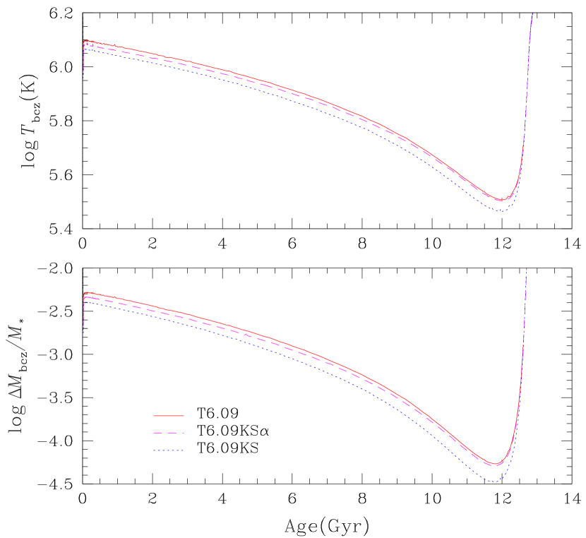
Figure 9: Mass in the surface convection zone and temperature at its bottom as a function of evolutionary time for a 0.8 $\,\mbox{\it M}_{\odot}$ model. The models differ by the boundary conditions and by the value of $\alpha$ used in the calculations. See Figure 6 and Table 2 for a definition of the notation used for models with turbulent transport.

Changing the surface boundary conditions has a significant effect on the depth of the surface convection zone (see Section 2.2 and Fig. 9). Two boundary conditions were used. Both are often used for Pop II models. In their solar models, Turcotte et al. (1998b) used mainly Krishna Swamy’s $T(\tau){}$ relation. It is used here for some series of models. Eddington’s $T(\tau){}$ relation is also used: it was used for A and F Pop I stars by Turcotte et al. (1998a) and Richer et al. (2000). In Turcotte et al. (1998b), the Sun is used to determine the appropriate value of $\alpha$ to use with each of these boundary conditions. One may view the difference in convection zone mass between the models (Fig. 9) as a reasonable estimate of the uncertainty. During evolution, the uncertainty varies from a factor of 1.3 to 1.6 in mass. This is sufficient to modify the fits to globular cluster isochrones (see Paper II). It has however a less pronounced effect on surface abundances than the uncertainty on turbulence. It modifies significantly surface abundances only when no turbulence is included in the models.

4 Surface abundances and observations

The surface concentrations of the 28 species impose constraints on stellar models. They will be shown for three series of models, the atomic diffusion models with no turbulence, those that mimic the turbulence of AmFm stars and those that minimize the effects of transport on surface Li concentration. Surface abundance variations as a function of time have been discussed above (see subsections 3.1 and  3.2). They are discussed below as a function of atomic number and of ${{T_{{{\mbox{\scriptsize eff}}}}}}$ in order to facilitate comparison to observations. In the first subsection, we present the results for all calculated species for individual stars. In the second subsection, we present results at a given age for stars of various masses as a function of ${{T_{{{\mbox{\scriptsize eff}}}}}}$. They are then compared to observations in the last subsection.

4.1 As a function of atomic number

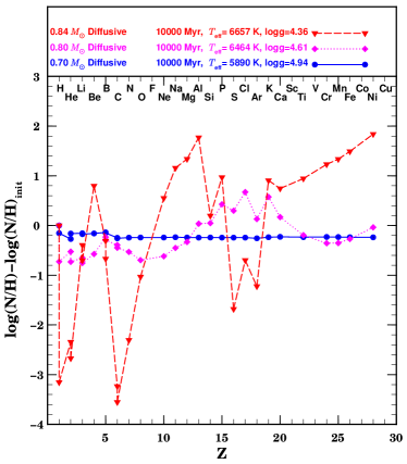
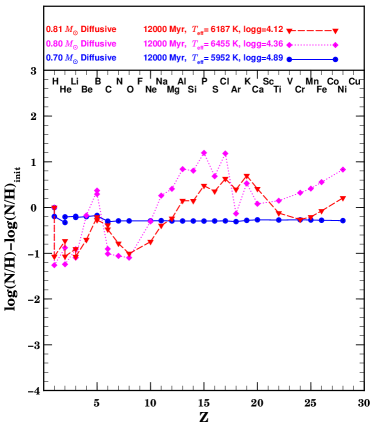
Figure 10: In the left hand panel, ratio of surface abundances to original abundances as a function of atomic mass in stars of 0.7, 0.8, and 0.84 $\,\mbox{\it M}_{\odot}$ after 10 Gyr of evolution. In the right hand panel, the 0.84 $\,\mbox{\it M}_{\odot}$ model is replaced by the 0.81 $\,\mbox{\it M}_{\odot}$ one and it is after 12 Gyr of evolution.

The surface concentrations at 10 and 12 Gyr are shown as a function atomic number in Figure 10 for the evolutionary models with atomic diffusion and no turbulence (see also subsection 3.1). The 0.7 $\,\mbox{\it M}_{\odot}$ model is the one with the smallest mass shown. In it, gravitational settling causes a general reduction of surface abundances by close to 0.2 dex. As may be seen from Figure 1, the convection zone is always at least 1% of the mass in a 0.7 $\,\mbox{\it M}_{\odot}$ star so that radiative accelerations play a modest role (see Fig. 2). In the 0.6 and 0.5 $\,\mbox{\it M}_{\odot}$ models (not shown), the mass in the surface convection zone is always larger than about 20 % of the stellar mass so that gravitational settling is negligible even after 10 or 12 Gyr.

In stars of 0.75 $\,\mbox{\it M}_{\odot}$ or more, the surface convection zone occupies less than 0.1 % of the stellar mass for part of the evolution. The $g_{{{\mbox{\scriptsize rad}}}}$ then play the major role for that part of the evolution. At 10 Gyr, the 0.8 $\,\mbox{\it M}_{\odot}$ model is significantly affected by $g_{{{\mbox{\scriptsize rad}}}}$ (see Fig. 10). The atomic species most affected are those between Al and Ca. They have overabundances by factors of up to 5. The Fe peak elements are hardly affected. In the 0.84 $\,\mbox{\it M}_{\odot}$ model, Ni is overabundant by a factor of 70, while Fe is overabundant by a factor of 30. Large underabundances are expected for CNO and Li while Be and B are supported at least partly by their $g_{{{\mbox{\scriptsize rad}}}}$. Since the original metallic abundances are small, the $g_{{{\mbox{\scriptsize rad}}}}$ are little affected by line saturation and the abundance anomalies reflect essentially the atomic configuration of the dominant ionization state of each chemical species. For instance, Li is completely stripped of its electrons while C, N and O are mainly in He-like configurations (see also Richer et al. 1998).

At 12 Gyr, the 0.84 $\,\mbox{\it M}_{\odot}$ model has already evolved to the giant phase. The most massive star around the turnoff has 0.81 $\,\mbox{\it M}_{\odot}$. It is already 300 K cooler than the turnoff so that its surface convection zone has already started to expand and its abundance anomalies to decrease. While its Fe peak shows approximately the original abundances, the species between Al and Ca have overabundances by up to a factor of 5. Note again that Be and B are supported by their $g_{{{\mbox{\scriptsize rad}}}}$ while Li has sunk. At that age, the 0.8 $\,\mbox{\it M}_{\odot}$ star is the star with the largest anomalies. Ni and species between Na and Cl are about a factor of 15 overabundant. He, Li and CNO are underabundant by a factor of about 10. At 12 Gyr, the 0.80 $\,\mbox{\it M}_{\odot}$ is at the peak of its abundance anomalies: its surface convection zone is just about to start getting deeper (see Fig. 1). The 0.7 $\,\mbox{\it M}_{\odot}$ star also has larger anomalies than at 10 Gyr. Its surface convection zone is still getting smaller (see Fig. 1) while the 20 % longer life means more time for gravitational settling.

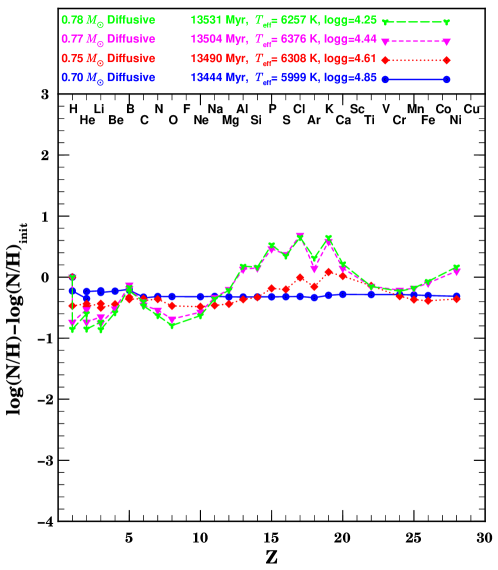
Figure 11: Ratio of surface abundances to original abundances as a function of atomic mass, after 13.5 Gyr of evolution, in 0.7, 0.75, 0.77 and 0.78 $\,\mbox{\it M}_{\odot}$ stars.

At 13.5 Gyr (the age of the oldest clusters as determined in Paper II) the surface abundances are shown in Figure 11 for stars with no turbulence. The lower mass star, 0.7 $\,\mbox{\it M}_{\odot}$, is at ${{T_{{{\mbox{\scriptsize eff}}}}}}=6000$ K and has seen its original abundances reduced by approximately 0.3 dex. This applies, in particular, to Li. The slightly warmer (6300 K) 0.75 $\,\mbox{\it M}_{\odot}$ star has a larger Li underabundance ($-$0.5 dex), marginally larger Fe peak underabundances ($-$0.39 dex) but the Ca abundance goes back to its original value because it is supported by its $g_{{{\mbox{\scriptsize rad}}}}$. Chemical species between Al and Ti are at least partially supported by their $g_{{{\mbox{\scriptsize rad}}}}$. The slightly more evolved 0.77 and 0.78 $\,\mbox{\it M}_{\odot}$ stars have nearly the same $T_{{{\mbox{\scriptsize eff}}}}$ but slightly lower gravities, less massive surface convection zones (see Fig. 1) and larger abundance anomalies than the 0.75 $\,\mbox{\it M}_{\odot}$ star. The two have very similar abundance anomalies. Fe has about its original abundance while species between Al and Ca have larger surface abundances than their original ones. Li is underabundant by a factor of 7.3. A comparison to Figure 10 shows that, for instance, Ni and Al abundance anomalies are reduced by a factor of 10 as one goes from clusters of 10 Gyr to clusters of 12 Gyr and then by a factor of 5 as one goes from clusters of 12 Gyr to clusters of 13.5 Gyr. As clusters age, the abundance anomalies caused by atomic diffusion in turnoff stars get progressively smaller.

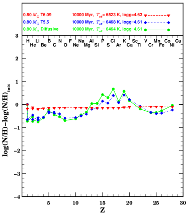
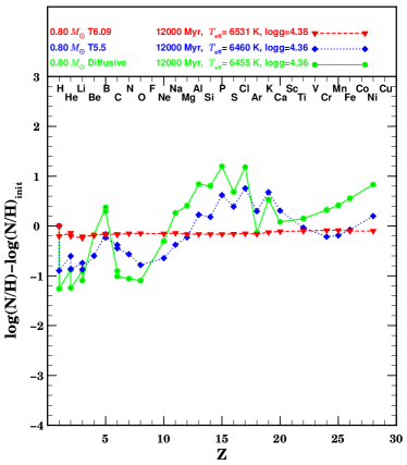
Figure 12: In the left/right hand panel, ratio of surface abundances to original abundances as a function of atomic mass in a 0.8 $\,\mbox{\it M}_{\odot}$ star, after 10/12 Gyr of evolution for 3 turbulence strengths: atomic diffusion only, the T5.5 and T6.09 turbulence models.

The effect of turbulence strength on surface composition is shown for the 0.8 $\,\mbox{\it M}_{\odot}$ model in Figure 12 at 10 and 12 Gyr. As a general rule, turbulence reduces abundance anomalies. However, in a 0.8 $\,\mbox{\it M}_{\odot}$ star, the effect of the T5.5D400-3 turbulence is more complex. Mg is mildly overabundant in the absence of turbulence but normal for the turbulence used, while Na goes from slightly over to slightly underabundant and the overabundance of Ca is increased by the increased turbulence. The anomalies between Al and Cl are more robust. These differences in behavior may be related to the differences in the internal distribution of the abundance variations caused by diffusion for various species (see Fig. 8). At 11.7 Gyr, species from Na to Cl have their maximum concentrations in the surface convection zone in the absence of turbulence. They are reduced by the extra mixing brought about by turbulence. However, Ar, K, Ca and Ti have their maximum concentrations below the convection zone so that some extra mixing increases their surface abundances. As a comparison with Figure 10 shows, the effect of adding turbulence is similar to that of considering a slightly more evolved, slightly more massive model (compare the 0.8 $\,\mbox{\it M}_{\odot}$ star with T5.5 of Fig. 12 with the 0.81 $\,\mbox{\it M}_{\odot}$ of Fig. 10), in that Fe peak anomalies are nearly eliminated in both while those between C and Ca are mildly reduced in both. The 0.78 $\,\mbox{\it M}_{\odot}$ no-turbulence model (not shown) has very similar surface concentrations as both the 0.81 $\,\mbox{\it M}_{\odot}$ model without turbulence and the 0.8 $\,\mbox{\it M}_{\odot}$ star with T5.5 turbulence. It differentiates itself by slightly larger N, O and F underabundances.

However, the mixing that is strong enough to minimize Li abundance variations (the T6.09 model) goes deeper than the region where $g_{{{\mbox{\scriptsize rad}}}}$ play a substantial role. Turbulence then reduces the abundance anomalies of all metals to 0.1$-$0.2 dex. All metals are underabundant if mixing is that strong.

4.2 As a function of ${{T_{{{\mbox{\scriptsize eff}}}}}}$.

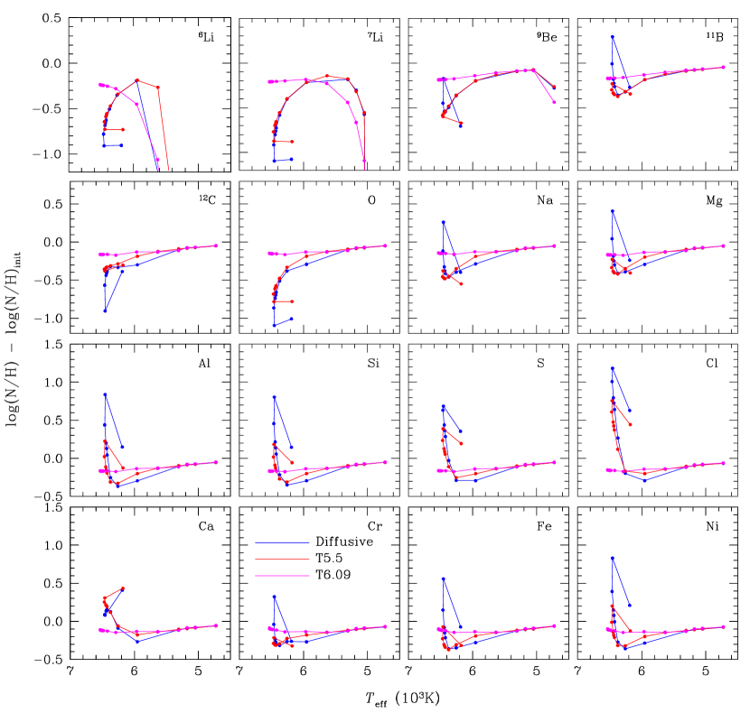
Figure 13: Ratio of surface to original abundances after 12 Gyr of evolution as a function of $T_{{{\mbox{\scriptsize eff}}}}$. The continuous line segments link models calculated with atomic diffusion. The dashed and dotted line segments link models calculated with atomic diffusion and, respectively, the T6.09 and T5.5 turbulence models.

The 12 Gyr surface abundance isochrones are shown as a function of ${{T_{{{\mbox{\scriptsize eff}}}}}}$ for a number of species (⁶Li, ⁷Li, Be, B, C, O, Na, Mg, Al, Si, S, Cl, Ca, Cr, Fe and Ni) in Figure 13 for the cases of atomic diffusion with no turbulence as well as with two turbulence strengths (T5.5 and T6.09). One first notes that, at the cool end, below 5000 K, there are only very small underabundances ($\leq 0.1$ dex) for all species and all turbulence strengths, except for Li which is destroyed by nuclear reactions and, to a lesser extent, Be. As one considers hotter stars, all underabundance factors increase until one reaches 6000 K. There the $g_{{{\mbox{\scriptsize rad}}}}$ start to play a role for some species. Furthermore, in the vicinity of the turnoff, stars of similar $T_{{{\mbox{\scriptsize eff}}}}$ have very different evolution states. In the absence of turbulence, some turnoff stars can have overabundances of Fe by up to 0.7 dex. Around the turnoff the Fe abundance can vary between $-$0.3 dex underabundance and 0.7 dex overabundance. The presence of even a very small amount of turbulence reduces this range by more than 0.7 dex (compare the continuous and dotted lines). The maximum abundance is reduced to the original Fe abundance while the underabundance factor is only slightly reduced to 0.25 dex. B, Mg, Cr, Mn and Ni are similarly affected by the same turbulence model though by slightly smaller factors. However the overabundances between P (not shown) and Ca are more robust. The range of Cl anomalies is merely reduced from a factor of 20 to a factor of about 7. Similarly, the large underabundances (He, Li, N and O; He and N are not shown) are not much reduced by the introduction of a small amount of turbulence. In a given cluster, the range of chemical species calculated then offers the possibility of testing turbulence models.

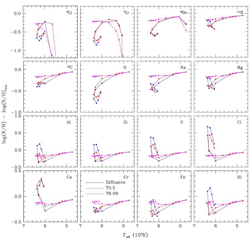
Figure 14: Ratio of surface to original abundances after 13.5 Gyr of evolution as a function of $T_{{{\mbox{\scriptsize eff}}}}$. The continuous line segments link models calculated with atomic diffusion. The dashed and dotted line segments link models calculated with atomic diffusion and, respectively, the T6.09 and T5.5 turbulence models.

The surface abundance isochrones at the age determined for M92 in Paper II are shown in Figure 14. One first notes, by comparing to Figure 13, the strong reduction in all abundance variations around the turnoff but the general slight increase in all underabundances in stars with ${{T_{{{\mbox{\scriptsize eff}}}}}}\leq 6000$ K. The increased underabundances reflect the increased time available for gravitational settling and the slight reduction in the depth of the surface convection zone between 12 and 13.5 Gyr (see Fig. 1).

At 13.5 Gyr, one then expects, in the absence of turbulence, underabundances of 0.05 dex at ${{T_{{{\mbox{\scriptsize eff}}}}}}{}=5000$ K increasing to 0.1 dex around 5500 K. Above that $T_{{{\mbox{\scriptsize eff}}}}$, underabundances remain approximately constant for stars with the T6.09 turbulence model. If there is no turbulence, underabundances increase to 0.3 dex at 6000 K and above that $T_{{{\mbox{\scriptsize eff}}}}$ both over and underabundances are present as $g_{{{\mbox{\scriptsize rad}}}}$ play a significant role. For the Fe peak elements, abundances are between the original and 0.3 dex underabundance. Only Ni could have an overabundance. Between C and Na all species are underabundant by a factor of order 2 while species between Al and Ca are generally overabundant. The presence of the T5.5 turbulence model mainly affects Al, Si, Fe and Ni overabundances which it reduces to or below the original abundance. Its presence is sufficient to reduce the expected range of underabundances of Fe to $-0.3\ldots-0.1$ dex.

5 Comparison to observations

Since in this paper results are presented only for stars with $Z=0.00017$, we will compare with the abundance determinations in M92 (see Boesgaard et al. 1998 and King et al. 1998). In so far as one may assume all cluster stars to share the same original composition, giant stars give a handle on the original turnoff star composition. The observations of clusters with larger $Z$ values will be discussed in a forthcoming paper where the evolutionary calculations for various values of $Z$ will be presented. We will use Li abundance in field halo stars with $Z\leq 0.001$ to complement the M92 observations. Since Li is believed to be of cosmological origin in these stars, one expects that the original abundance is the same for all.

The ${}^{7}\mbox{Li}$ observations of Spite & Spite (1982) and Spite et al. (1984), who have established the presence of a Li abundance plateau, are compared in Figure 15 to ${}^{7}\mbox{Li}$ abundance isochrones at the age of M92 (13.5 Gyr) and at 12 Gyr. The observations of Ryan et al. (1999), are also included since they further constrain the high $T$ part of the plateau. Given these results, it appears difficult to question the constraints imposed by the Li plateau, as done by Salaris & Weiss (2001). Results for 3 series of models are shown: those with atomic diffusion without turbulence and those with the T5.5 and T6.09 turbulent transport models. The stars calculated with the T6.09 model clearly fit the ${}^{7}\mbox{Li}$ observations much better. Both at 12 and 13.5 Gyr, there is a uniform ${}^{7}\mbox{Li}$ abundance extending from ${{T_{{{\mbox{\scriptsize eff}}}}}}=5500$ to 6000 K, in agreement with observations. It corresponds to an underabundance by 0.17 dex from the original Li abundance. Note also that ${}^{6}\mbox{Li}$ is reduced by less than a factor of 2 in turnoff stars (see Fig. 13 and Fig. 14), which is compatible with the observations of the presence of ${}^{6}\mbox{Li}$ in those Pop II objects (see Cayrel et al. 1999).

The series of models calculated without turbulence and that calculated with the T5.5 model do not reproduce the observations for ${{T_{{{\mbox{\scriptsize eff}}}}}}\geq 6100$ K. Given the observational error bars, the T6.09 model leads to a $T_{{{\mbox{\scriptsize eff}}}}$ dependence of $X$(Li) which is perhaps more constant than required. However, at 12 Gyr, calculations with the T6.0 model (not shown) give a Li abundance 0.15 dex smaller at 6500 K than at 5600 K. While perhaps compatible with the error bars, this would lead to a significantly poorer fit and may be considered the lower limit to the turbulent transport required by observations.

The lithium abundances observed in the M92 turnoff stars by Boesgaard et al. (1998) are also shown in the 13.5 Gyr part of the figure. The error bars are much larger than for field stars mainly because of the much smaller signal to noise ratio. The determined Li abundances suggest a slightly larger original value for the Li abundance in M92 than in halo stars but, given the size of the error bars, this could be considered uncertain. One star has a Li abundance higher than the others by a factor larger than the error bars. Other stars at the same $T_{{{\mbox{\scriptsize eff}}}}$ have a clearly smaller equivalent width of the Li doublet. The authors used this to argue for Li destruction by a large factor in Pop II stars. This appears premature to us.

King et al. (1998) have observed 7 metals mainly in three subgiant stars of M92 with ${{T_{{{\mbox{\scriptsize eff}}}}}}\simeq 6020$ K (see their discussion of $T_{{{\mbox{\scriptsize eff}}}}$ in their section 4.3), which is slightly cooler than our 6300 K turnoff $T_{{{\mbox{\scriptsize eff}}}}$ at 13.5 Gyr. Their determination of the Fe abundance is based on more lines and appears more reliable than that of other metals. It is the only metal we discuss. Their main conclusion is that the subgiants of M92 have a 0.26 dex lower Fe abundance than the giants of M92 as determined by Sneden et al. (1991). They carefully discuss all sources of error and cannot completely exclude that this 0.26 dex difference be reduced even possibly to zero. If the T6.09 turbulent transport model applies, all 3 stars should have the same Fe abundance and it should be approximately 0.1 dex smaller than the original Fe abundance according to our Figure 14. The giants should have the original Fe abundance because of their large surface convection zones. This seems quite compatible with the observations of Fe given the uncertainties.

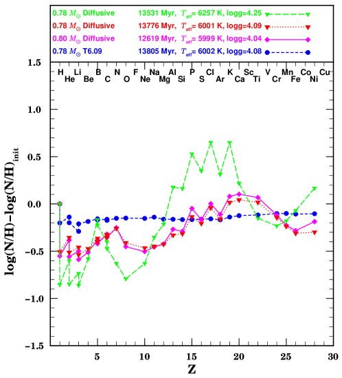
Figure 17: Surface abundances at ${{T_{{{\mbox{\scriptsize eff}}}}}}=6000$K for a 0.8 and a 0.78 $\,\mbox{\it M}_{\odot}$ star with atomic diffusion only. Their ages bracket the age of M92, 13.5 Gyr. Both stars have very closely the same composition showing that surface abundances are not a sensitive function of mass at ${{T_{{{\mbox{\scriptsize eff}}}}}}=6000$K, when the star is on the subgiant branch. A 0.78 $\,\mbox{\it M}_{\odot}$ star with the T6.09 turbulence model is also shown at the same $T_{{{\mbox{\scriptsize eff}}}}$. Finally the 0.78 $\,\mbox{\it M}_{\odot}$ star with no turbulence is shown at 13.5 Gyr when it is a turnoff star (${{T_{{{\mbox{\scriptsize eff}}}}}}=6250$K).

King et al. (1998) also find (their section 4.2) that star 21 has a 0.15 dex larger Fe abundance than the other two (stars 18 and 46). Furthermore Boesgaard et al. (1998) observed that the ⁷Li abundance is a factor of 3 smaller in star 21 than in star 18. This is to be compared to our results in Figure 14. At the turnoff, the Li and Fe abundances are sensitive functions of both the exact evolutionary state and turbulence. At 13.5 Gyr, in 0.78 $\,\mbox{\it M}_{\odot}$ models without turbulence, the Fe abundance is $-$0.05 dex from normal. Introducing the T5.5 turbulence model reduces it by 0.25 dex while the T6.09 model brings it back to $-$0.1 dex from normal. As may be seen in Figure 16, the Fe abundance as a function of $T_{{{\mbox{\scriptsize eff}}}}$ has a complex loop structure around the turnoff in both 0.8 and 0.78 $\,\mbox{\it M}_{\odot}$ stars. Small changes in evolutionary state and/or turbulence can change the Fe abundance by 0.2$-$0.3 dex and the ⁷Li abundance by 0.5$-$0.6 dex. At the turnoff, the different Li and Fe abundances would then be explained by a different turbulence between the stars, resolving the difficulty described in Section 4.2 of King et al. (1998). They would become the Pop II analogue of AmFm stars. However all three of those stars appear to be past the turnoff. As Figure 16 shows, the $g_{{{\mbox{\scriptsize rad}}}}$ have significant effects on surface abundances in stars of mass 0.77 $\,\mbox{\it M}_{\odot}$ and more but, for Fe, these effects are limited to ${{T_{{{\mbox{\scriptsize eff}}}}}}\geq 6100$ K. As seen in Figure 17, the abundance variations at the turnoff are not expected in subgiants when they reach 6020 K. At this temperature, reducing turbulence leads to more gravitational settling for both Li and Fe which cannot explain the differences between stars 18 and 21. While turnoff stars of a cluster could have abundance variations as observed for stars 18, 21 and 46, these are not expected in stars with exactly the parameters determined for them—and this is a difficulty even if there appears to be considerable uncertainty in the $T_{{{\mbox{\scriptsize eff}}}}$ of stars in this cluster (compare the $T_{{{\mbox{\scriptsize eff}}}}$ of Carney 1983 to those of King 1993 and the discussion in Section 4.3 of King et al. 1998). Note that in the comparison to our evolutionary models, it is the absolute $T_{{{\mbox{\scriptsize eff}}}}$ scale that matters and not just the $T_{{{\mbox{\scriptsize eff}}}}$ with respect to the turnoff $T_{{{\mbox{\scriptsize eff}}}}$. If anomalies are confirmed, agreement with our model would require the higher $T_{{{\mbox{\scriptsize eff}}}}$ scale for M92.

6 Conclusion

It has been clearly shown that, contrary to the belief expressed in many papers and recently by Chaboyer et al. (2001), atomic diffusion does not necessarily lead to underabundances of metals in Pop II stars. Differential radiative accelerations lead to overabundances of Fe and some other chemical elements in some turnoff stars.

Consider the evolution of Pop II stars with no tubulence. As one may see by considering the solid curves in Figures 13 and 14, generalized underabundances by 0.1 dex are expected in the $T_{{{\mbox{\scriptsize eff}}}}$ interval from 4600 to 5500  K. Between 5500 and 6000  K, the underabundances are still generalized and increase to 0.3 dex for some species such as O. In 12 Gyr turnoff stars however (${{T_{{{\mbox{\scriptsize eff}}}}}}{}\geq 6000$  K), overabundances by a factor of up to 10 are possible (e.g. Al and Ni). All calculated species heavier than Na may have overabundances. At a given $T_{{{\mbox{\scriptsize eff}}}}$, variations are expected from star to star. At 13.5 Gyr, similar but smaller anomalies are expected. The overabundances are sensitive to any left over turbulence below the convection zone.

In this paper, the evolution of stars with $Z=0.00017$ has been described both with and without turbulence. A 0.1 dex underabundance of metals in turnoff stars as compared to giants has been shown to be the smallest anomaly to be expected (section 4.2). Star– to– star variations were seen to be possible around the turnoff, if turbulence is small enough. Observations (see section 5) suggest the presence of abundance variations similar to those expected. The comparison to observations is, however, sensitive to the $T_{{{\mbox{\scriptsize eff}}}}$ scale. As King et al. (1998) concluded at the end of their section 4.2, higher quality data is probably required to establish the reality of Fe abundance variations within M92. The accurate determination of the abundance of more species is also needed. This may well have implications not only for intrinsic abundance variations in clusters but for internal stellar structure.

The effect of varying $Z$ on the evolution of Pop II stars will be investigated in a forthcoming paper, (Paper III), where comparisons to higher $Z$ clusters will be undertaken. Increasing $Z$ in Pop II stars will be shown to reduce considerably the expected abundance anomalies. Note also that Paper II shows that the present models for $[\mbox{Fe}/\mbox{H}]_{0}=-1.31$ accurately reproduce the CMD locations of local Population II subdwarfs having Hipparcos parallaxes and metallicities within +/$-$ 0.2 dex of $[\mbox{Fe}/\mbox{H}]=-1.3$.

In a number of clusters with higher $Z$ than M92, observations suggest that only small variations, if any, are present in turnoff stars (see for instance Ramirez et al. 2001; Gratton et al. 2001 and Thévenin et al. 2001). Furthermore in field halo stars, the Li abundance puts strict constraints on any chemical separation. In the companion paper (Paper II) we therefore took the cautious approach to use mainly evolutionary models that minimize the effect of atomic diffusion.

It has been shown that the use, in complete stellar evolution models, of a relatively simple parametrization of turbulent transport leads to Li surface abundances compatible with the Li plateau observed in field halo stars (with a 0.17 dex reduction from the original Li abundance) and small variations in the surface abundances of metals (a 0.1 dex reduction of the metal abundance in turnoff stars as compared to that in giants in clusters with $Z=0.00017$). At the same time, the gravitational settling of He leads to a reduction in the age of globular clusters by some 10 % (see Paper II). However simple the parametrization of turbulent transport, it is not understood from first principles. The high level of constancy of Li abundance as a function of $T_{{{\mbox{\scriptsize eff}}}}$ requires that turbulence mixes to very nearly the same $T$ throughout the star evolution and in stars covering a mass interval of approximately 0.6 to 0.8 $\,\mbox{\it M}_{\odot}$. As already noted by Michaud et al. (1984), this is not expected in standard stellar models. No convincing hydrodynamic model has been proposed that explains this property. Pop II stars appear to tell us that this is the case, however.

Mass loss is another physical process that could compete with atomic diffusion and maintain a constant value of Li as a function of $T_{{{\mbox{\scriptsize eff}}}}$ (Vauclair & Charbonnel, 1995). Whether, in the absence of turbulent transport, it could be made consistent with the observations of metals in globular cluster turnoff stars is a question that requires further calculations. These may lead to observational tests of the relative importance of mass loss and turbulence in these objects. The number of chemical species that are now included in these calculations and that can be observed makes such tests possible.

Table 1: Initial chemical composition

Element	Note	Mass fraction
		[Fe/H]=-2.31	[Fe/H]=-1.31
H		7.646$\times 10^{-1}$	7.613$\times 10^{-1}$
4He		2.352$\times 10^{-1}$	2.370$\times 10^{-1}$
12C		1.727$\times 10^{-5}$	1.727$\times 10^{-4}$
N		5.294$\times 10^{-6}$	5.294$\times 10^{-5}$
O		9.612$\times 10^{-5}$	9.612$\times 10^{-4}$
Ne		1.966$\times 10^{-5}$	1.966$\times 10^{-4}$
Na		3.986$\times 10^{-7}$	3.986$\times 10^{-6}$
Mg		7.484$\times 10^{-6}$	7.484$\times 10^{-5}$
Al		1.627$\times 10^{-7}$	1.627$\times 10^{-6}$
Si		8.072$\times 10^{-6}$	8.072$\times 10^{-5}$
P		6.976$\times 10^{-8}$	6.976$\times 10^{-7}$
S		4.215$\times 10^{-6}$	4.215$\times 10^{-5}$
Cl		8.969$\times 10^{-8}$	8.969$\times 10^{-7}$
Ar		1.076$\times 10^{-6}$	1.076$\times 10^{-5}$
K		1.998$\times 10^{-8}$	1.998$\times 10^{-7}$
Ca		7.474$\times 10^{-7}$	7.474$\times 10^{-6}$
Ti		3.986$\times 10^{-8}$	3.986$\times 10^{-7}$
Cr		9.989$\times 10^{-8}$	9.989$\times 10^{-7}$
Mn		3.890$\times 10^{-8}$	3.890$\times 10^{-7}$
Fe		7.172$\times 10^{-6}$	7.172$\times 10^{-5}$
Ni		4.445$\times 10^{-7}$	4.445$\times 10^{-6}$
Z		1.675$\times 10^{-4}$	1.675$\times 10^{-3}$

Table 2: Parameters used for the different series of models identified in the first column

Series name	Boundary condition	$\alpha{}$	[Fe/H]	Diffusion and	Turbulence
				radiative accelerations
Non-diffusive	Eddington	1.687	$-2.31$	no	no
Diffusive	Eddington	1.687	$-2.31$	yes	no
T5.5	Eddington	1.687	$-2.31$	yes	T5.5D400-3
T6.0	Eddington	1.687	$-2.31$	yes	T6.0D400-3
T6.09	Eddington	1.687	$-2.31$	yes	T6.09D400-3
T6.13	Eddington	1.687	$-2.31$	yes	T6.13D400-3
T6.09KS	Krishna-Swamy	1.869	$-2.31$	yes	T6.09D400-3
T6.09KS$\alpha$	Krishna-Swamy	2.017	$-2.31$	yes	T6.09D400-3
Non-diffusive$-1.31$	Eddington	1.687	$-1.31$	no	no
Diffusive$-1.31$	Eddington	1.687	$-1.31$	yes	no
T6.0$-1.31$	Eddington	1.687	$-1.31$	yes	T6.00D400-3
T6.09$-1.31$	Eddington	1.687	$-1.31$	yes	T6.09D400-3

References

- Bahcall et al. (1995) Bahcall, J. N., Pinsonneault, M. H., & Wasserburg, G. J. 1995, Rev. Mod. Phys., 67, 781
- Basu (1997) Basu, S. 1997, MNRAS, 288, 572
- Bell et al. (2001) Bell, R. A., Balachandran, S. C., & Bautista, M. 2001, ApJ, 546, L65
- Boesgaard et al. (1999) Boesgaard, A. M., Deliyannis, C. P., King, J. R., Ryan, J. R., Vogt, S. S., & Beers, T. C. 1999, AJ, 117, 1549
- Boesgaard et al. (1998) Boesgaard, A. M., Deliyannis, C. P., Stephens, A., & King, J. R. 1998, ApJ, 493, 206
- Brun et al. (1999) Brun, A. S., Turck-Chieze, S., & Zahn, J. P. 1999, ApJ, 525, 1032
- Carney (1983) Carney, B. W. 1983, AJ, 88, 610
- Cayrel (1998) Cayrel, R. 1998, Space Science Reviews, 84, 145
- Cayrel et al. (1999) Cayrel, R., Spite, M., Spite, F., & Audouze, J. 1999, A&A, 343, 923
- Chaboyer et al. (2001) Chaboyer, B., Fenton, W. H., Nelan, J. E., Patnaude, D. J., & Simon, F. E. 2001, ApJ, in press
- Christensen-Dalsgaard et al. (1993) Christensen-Dalsgaard, J., Proffitt, C. R., & Thompson, M. J. 1993, ApJ, 403, 75
- Deliyannis et al. (1990) Deliyannis, C. P., Demarque, P., & Kawaler, S. D. 1990, ApJS, 73, 21
- Freytag & Salaris (1999) Freytag, B. & Salaris, M. 1999, ApJ, 513, L49
- Gonzalez et al. (1995) Gonzalez, J.-F., LeBlanc, F., Artru, M.-C., & Michaud, G. 1995, A&A, 297, 223
- Gratton et al. (2001) Gratton, R. G., Bonifacio, P., Bragaglia, A., Carretta, E., Castellani, V., Centurion, M., Chieffi, A., Claudi, R., Clementini, G., D’Antona, F., Desidera, S., François, P., Grundahl, F., Lucatello, S., Molaro, P., Pasquini, L., Sneden, C., Spite, F., & Straniero, O. 2001, A&A, 369, 87
- Guenther et al. (1996) Guenther, D. B., Kim, Y.-C., & Demarque, P. 1996, ApJ, 463, 382
- Guzik & Cox (1992) Guzik, J. A. & Cox, A. N. 1992, ApJ, 386, 729
- Guzik & Cox (1993) —. 1993, ApJ, 411, 394
- Hobbs & Thorburn (1994) Hobbs, L. M. & Thorburn, J. A. 1994, ApJ, 428, L25
- Hobbs & Thorburn (1997) —. 1997, ApJ, 491, 772
- King (1993) King, J. R. 1993, AJ, 106, 1206
- King et al. (1998) King, J. R., Stephens, A., Boesgaard, A. M., & Deliyannis, C. F. 1998, AJ, 115, 666
- Krishna Swamy (1966) Krishna Swamy, K. S. 1966, ApJ, 145, 174
- LeBlanc et al. (2000) LeBlanc, F., Michaud, G., & Richer, J. 2000, ApJ, 538, 876
- Lumer et al. (1990) Lumer, E., Forestini, M., & Arnould, M. 1990, A&A, 240, 515
- Michaud (1991) Michaud, G. 1991, Ann. Phys. (Paris), 16, 481
- Michaud et al. (1984) Michaud, G., Fontaine, G., & Beaudet, G. 1984, ApJ, 282, 206
- Michaud & Proffitt (1993) Michaud, G. & Proffitt, C. R. 1993, in Inside the Stars, IAU COLLOQUIUM 137, Vienna, April 1992, ASP Conference Series, 40, ed. W. W. Weiss & A. Baglin (San Francisco: ASP), 246
- Molaro & Pasquini (1994) Molaro, P. & Pasquini, L. 1994, A&A, 281, L77
- Paquette et al. (1986) Paquette, C., Pelletier, C., Fontaine, G., & Michaud, G. 1986, ApJS, 61, 177
- Pinsonneault et al. (1999) Pinsonneault, M. H., Walker, T. P., Steigman, G., & Narayanan, V. K. 1999, ApJ, 527, 180
- Proffitt (1994) Proffitt, C. R. 1994, ApJ, 425, 849
- Proffitt & Michaud (1991a) Proffitt, C. R. & Michaud, G. 1991a, ApJ, 371, 584
- Proffitt & Michaud (1991b) —. 1991b, ApJ, 380, 238
- Proffitt & VandenBerg (1991) Proffitt, C. R. & VandenBerg, D. A. 1991, ApJS, 77, 473
- Ramaty et al. (2000) Ramaty, R., Tatischeff, V., Thibaud, J. P., Kozlovsky, B., & Mandzhavidze, N. 2000, ApJ, 534, L207
- Ramirez et al. (2001) Ramirez, S. V., Cohen, J. G., Buss, J., & Briley, M. M. 2001, AJ, 122, 1429
- Richard et al. (2001) Richard, O., Michaud, G., & Richer, J. 2001, ApJ, 558, 377
- Richard et al. (1996) Richard, O., Vauclair, S., Charbonnel, C., & Dziembowski, W. A. 1996, A&A, 312, 1000
- Richer et al. (1998) Richer, J., Michaud, G., Rogers, F., Iglesias, C., Turcotte, S., & LeBlanc, F. 1998, ApJ, 492, 833
- Richer et al. (2000) Richer, J., Michaud, G., & Turcotte, S. 2000, ApJ, 529, 338
- Ryan et al. (1999) Ryan, S. G., Norris, J. E., & Beers, T. C. 1999, ApJ, 523, 654
- Salaris et al. (2000) Salaris, M., Groenewegen, M. A. T., & Weiss, A. 2000, A&A, 355, 299
- Salaris & Weiss (2001) Salaris, M. & Weiss, A. 2001, A&A, 376, 955
- Smith et al. (1993) Smith, V. V., Lambert, D. L., & Nissen, P. E. 1993, ApJ, 408, 262
- Sneden et al. (1991) Sneden, C., Kraft, R. P., Prosser, C. F., & Langer, G. E. 1991, AJ, 102, 2001
- Spite & Spite (1982) Spite, F. & Spite, M. 1982, A&A, 115, 357
- Spite et al. (1984) Spite, M., Maillard, J.-P., & Spite, F. 1984, A&A, 141, 56
- Stringfellow et al. (1983) Stringfellow, G. S., Bodenheimer, P., Noerdlinger, P. D., & Arigo, R. J. 1983, ApJ, 264, 228
- Thévenin et al. (2001) Thévenin, F., Charbonnel, C., de Freitas Pacheco, J. A., Idiart, T. P., Jasniewicz, G., de Laverny, P., & Plez, B. 2001, A&A, 373, 905
- Turcotte et al. (1998a) Turcotte, S., Richer, J., & Michaud, G. 1998a, ApJ, 504, 559
- Turcotte et al. (1998b) Turcotte, S., Richer, J., Michaud, G., Iglesias, C., & Rogers, F. 1998b, ApJ, 504, 539
- VandenBerg et al. (2001) VandenBerg, D. A., Richard, O., Michaud, G., & Richer, J. 2001, ApJ
- VandenBerg et al. (2000) VandenBerg, D. A., Swenson, F. J., Rogers, F. J., Iglesias, C. A., & Alexander, D. R. 2000, ApJ, 532, 430
- Vauclair (1988) Vauclair, S. 1988, ApJ, 335, 971
- Vauclair & Charbonnel (1995) Vauclair, S. & Charbonnel, C. 1995, A&A, 295, 715