Caught in the Act; Chandra Observations of Microlensing of the Radio-Loud Quasar MG J0414+0534
Abstract
We present results from monitoring of the distant (z = 2.64), gravitationally lensed quasar MG J0414+0534 with the Chandra X-ray Observatory. An Fe K line at 6.49 0.09 keV (rest-frame) with an equivalent width of 190 eV consistent with fluorescence from a cold medium is detected at the 99% confidence level in the spectrum of the brightest image A. During the last two observations of our monitoring program we detected a five-fold increase of the equivalent width of a narrow Fe K line in the spectrum of image B but not in the brighter image A whereas image C is too faint to resolve the line. The continuum emission component of image B did not follow the sudden enhancement of the iron line in the last two observations. We propose that the sudden increase in the iron line strength from 190 eV to 900 eV only in image B can be explained with a caustic crossing due to microlensing that selectively enhances a strip of the line emission region of the accretion disk. The non-enhancement of the continuum emission in the spectrum of image B suggests that the continuum emission region is concentrated closer to the center of the accretion disk than the iron line emission region and the magnification caustic has not reached close enough to the former region to amplify it. A model of a caustic crossing event predicts discontinuities in the light-curve of the magnification and provides an upper limit of 5 10-4 pc on the outer radius of the Fe K emission region. The non-detection of any relativistic or Doppler shifts of the iron line in the spectrum of image B implies that the magnification caustic for the last two observations was located at a radius greater than 100 gravitational radii.
Each observation of the quadruply lensed quasar MG J0414+0534 provides a view of the quasar at four different epochs spaced by the time-delays between the lensed images. We produced a light-curve of the quasar X-ray flux by normalizing the flux of each image to the mean flux of that image over all observations. We find significant deviations of the normalized light-curve from unity especially for the faintest image C. A plausible mechanism to explain the flux variability of image C is a microlensing event. Finally, spectral analysis of MG J0414+0534 indicates the presence of significant absorption in excess of the Galactic value. For absorption at the redshift of the lensed quasar we find an intrinsic column density of NH 5 1022 cm-2, consistent with the reddening observed in the optical band.
Subject headings:
gravitational lensing — accretion disks — X-rays: general — quasars: individual (MG J0414+0534)1. INTRODUCTION
Direct imaging of the immediate environments of black holes in Active Galactic Nuclei (AGNs) is beyond the capabilities of present day telescopes; rough estimates of the characteristic sizes of emission regions of AGN in the radio, optical and X-ray bands, based on light-travel time arguments, correspond to angular sizes on the order of tens of nano-arcseconds at a redshift of . However, indirect mapping methods have been developed recently to study the environs of AGN without the need of nano-arcsec resolution. One of these methods, known as reverberation mapping (Blandford & McKee 1982), has been successfully used to determine the size and probe the structure of the broad-line region in several AGN (see Peterson 1993 and Netzer & Peterson 1997 for recent reviews). This method relies on the time lag between variations in the flux from a central source of ionizing radiation and the response of the emission lines from photo-ionized gas in the broad-line region. A closely related technique for indirect mapping of the accretion disk around the black hole relies on the variation of the profiles of the Fe K fluorescence lines originating in the inner parts of the disk. The line profiles are determined by a combination of the Doppler effect and special and general relativistic effects (e.g., Fabian et al 1989; Laor 1991) while their variations are caused by fluctuations in the X-ray continuum that drive the line emission (Young & Reynolds 2000).
A recently proposed, independent, method for indirect imaging of AGN accretion disks exploits the high-magnification microlensing events (HMEs) in gravitational lens (GL) quasars (Grieger et al. 1988 and 1991; Schneider, Ehlers & Falco 1992; Gould & Gaudi 1997; Agol & Krolik 1999; Yonehara et al. 1999; Mineshige & Yonehara 1999, Yonehara 2001; Shalyapin 2001). During a microlensing event magnification caustics produced by stars in the lensing galaxy traverse the plane of the accretion disk and selectively magnify different emission regions. An analysis of the light-curves of microlensing events obtained in several wavelengths can be used to infer the surface brightness and inclination angle of the accretion disk and possibly provide constraints on the mass and spin of the black hole (e.g, Agol & Krolik 1999 and references within). A promising object for application of this technique is the Einstein Cross. With the first detection of a microlensing event in the Einstein Cross by Irwin et al. (1989) and subsequent verification by Corrigan et al. (1991) and Ostensen et al. (1996) it became clear that future monitoring of the Einstein Cross has the potential of yielding information on the geometry of the accretion disk and possibly the spin and mass of the black hole. Thus, a program to monitor magnification events in the Einstein Cross has been undertaken as part of the Optical Gravitational Lensing Experiment (OGLE, see Woźniak et al. 1999 and references within). Microlensing events have been detected with OGLE, however a clear case of a HME due to a caustic crossing has yet to be detected. Recently, constraints on the continuum source size of the lensed quasar have been derived based on the microlensing light-curves of the Einstein Cross (eg., Wyithe, Webster & Turner 2000; Yonehara 2001; Shalyapin 2001).
In this paper we report the serendipitous detection of significant variations in the shape and equivalent width (EW) of a reprocessed Fe K line only in one of the lensed images of the quasar MG J0414+0534. We interpret this change as the result of the crossing of the accretion disk by a magnification caustic.
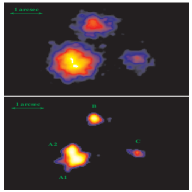
The gravitational lens system MG J0414+0534 was discovered by Hewitt et al. (1992). The system consists of four lensed images commonly referred to as A1, A2, B and C (see Figure 1) with the separation between A1 and A2 being 04. The lensed source is a distant (z = 2.639), low-luminosity radio quasar (Lawrence et al. 1995). A faint blue arc is detected in HST observations (Falco et al. 1997) that extends between images A1 and B. The arc is most likely the host galaxy of the quasar lensed by the foreground elliptical galaxy located at a redshift of 0.96 (Tonry & Kochanek 1999). An object located 1 ″ West of image B and referred to as object X (Schechter & Moore 1993) possibly contributes to the lensing effect. IR observations of MG J0414+0532 indicate that the components of this system are exceedingly red with respective R-H colors of 6.8 mag for image C, 3.2 mag for the arc, and 3.2 mag for the lens galaxy. The origin of the absorption is controversial with early studies mostly favoring the dusty lens hypothesis (Lawrence et al. 1995; Malhotra, Rhoad, & Turner 1997; McLeod et al. 1998) and more recent work suggesting a host galaxy origin (Tonry & Kochanek 1999; Falco et al. 1997) or a combination of lens and host (Angonin-Willaime et al. 1999). The flux ratios have been observed to be a function of wavelength and this has been interpreted as either due to extinction in the lens or microlensing of one or more of the images. Recent VLBI and HST NICMOS H-band images have been used to produce accurate lens models for this system (Ros et al. 2000). These models predict the time delays between the lensed images to be 16 1.4 days and 66 5 days. The time-delays predicted from the lens model of Ros et al. (2000) assume a flat cosmology with and km s-1 Mpc-1. The monitoring program of MG J0414+0532 with Chandra was planned such that the time interval between observations was substantially shorter than a year, roughly the predicted average rise for a high magnification event due to microlensing in this GL system (Witt, Mao & Schechter 1995). A detailed description of the Chandra observations of MG J0414+0534 and the data reduction procedures used is presented in section 2. The resolved X-ray lensed images of this GL system are presented in section 3. The spectral analysis revealing the properties of an intervening absorber and reprocessed iron line features is detailed in section 4. We conclude with a discussion of the origin of the detected iron line features and the prospects of mapping the accretion disk of a distant quasar with microlensing of a reprocessed Fe K line.
2. OBSERVATION AND DATA REDUCTION
MG J0414+0534 was observed with the Advanced CCD Imaging spectrometer (ACIS) instrument (G. P. Garmire et al. 2002, in preparation) onboard the Chandra X-ray Observatory (CXO) in a series of five pointings listed in Table 1. The pointing of the telescope placed MG J0414+0534 on the back-illuminated S3 chip of ACIS.
The observations were performed as part of a survey of GL systems with the CXO aimed at finding suitable candidates for time-delay measurements. The software package CIAO 2 provided by the Chandra X-ray Center was used to process the data. We chose to remove a 025 randomization applied to the event positions in the CXC processing. The randomization is used in the standard CXC pipeline processing to deal with aliasing effects noticed in observations with durations of less than 4 ks. Removal of the pixel randomization results in an improvement of the spatial resolving power by about 01. To improve the spatial resolution of ACIS even further we employed a method recently developed by Tsunemi et al. (2001). The physical basis of this method is as follows; Any photon that is detected by ACIS produces a charge cloud of electrons that is collected by one or more pixels. The different arrangements of charge are referred to as ACIS grade distributions. Particular grade distributions often referred to as corner events can be used to locate the position of the incident photons to sub-pixel accuracy. By correcting the positions of corner pixel events the spatial resolution of ACIS is significantly improved.
3. RELATIVE ASTROMETRY AND PHOTOMETRY
The Chandra image of MG J0414+0534 obtained from combining the five observations
listed in Table 1 is presented in Figure 1.
Images A1 and A2 are not clearly resolved in the Chandra image.
We applied the Lucy - Richardson (L-R) maximum likelihood
deconvolution technique to improve the image quality. L-R
deconvolution was applied to the combined image of the five
observations of MG J0414+0534. For the deconvolution we supplied a
point spread function (PSF) created by the simulation tool MARX (Wise
et al. 1997). The X-ray spectrum used to generate the PSF was that
determined from our spectral analysis of the combined images of
MG J0414+0534. In particular, we used an absorbed power-law model with
absorption of NH = 10.85 1020 cm-2 due to our
Galaxy, intrinsic absorption at z = 2.64 of NH = 4.76
1022 cm-2 , and a photon index of 1.72. In Figure 1 we
present the original and deconvolved image of the combined
observations. In Table 1 we provide the epochs, exposure times and
detected events for the lensed images for each observation of
MG J0414+0534. In Table 2 we present the relative X-ray and optical
(HST) positions of MG J0414+0534 images A1, A2, and B with respect to
image C. We find a good agreement between optical and X-ray positions.
The detected count rates of images A1+A2, B, and C versus Julian date are shown in Figure 2. Figure 2 also shows the X-ray flux ratios A/B, A1/A2 and C/B for each observation. These flux ratios are not phase-corrected for the predicted time-delays. The flux ratios A/B and C/B were derived by extracting events from circles of radii 1 ″ centered on the images. Due to the close separation between images A1 and A2 of 04 we estimated the X-ray flux ratio A1/A2 by performing a likelihood analysis on the binned event positions; We modeled A1 and A2 with simulated PSF’s and minimized the Cash (1979) C statistic formed between the observed and predicted events to find the best fit normalization values. The relative positions of A1 and A2 were held fixed to the optical positions listed in Table 2. For the 5th observation of MG J0414+0534 with the highest signal-to-noise ratio we obtain a A1/A2 X-ray flux ratio of 1.3 0.2 which is consistent within the uncertainties to the radio flux ratio of 1.1. In Table 3 we present the 8GHz (Katz, Moore, Hewitt 1997), the H, R, and I band (CfA-Arizona Space Telescope LEns Survey (CASTLES)) and the 2-8keV band flux ratios of the components of MG J0414+0534.
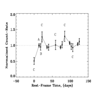
For a comparison with other observations we have included in Figure 2 the HST values of the flux ratios obtained in the optical H-band. In Figure 3 we present the Chandra light-curve of MG J0414+0534. The count-rates of each image have been normalized to the average count-rate of that image for the five observations listed in Table 1. Based on the lens models of Ros et al. (2000) we assume that image B leads images A and C by 16 and 66 days, respectively. Long term variability is significant for image C and not in the other images suggesting that microlensing may be present in image C. The double peaked light-curve of MG J0414+0534 is suggestive of a double-caustic crossing event in image C.
4. SPECTRAL ANALYSIS
We performed spectral analysis for each
observation of MG J0414+0534 listed in Table 1.
A variety of spectral models were fitted to the data
employing the software tool XSPEC v11 (Arnaud 1996).
The spectra of images A, B, and C were extracted from circular regions
centered on the images with radii of 1 ″.
The background was determined by extracting events within an
annulus centered on the midpoint between images A and B and
with inner and outer radii of 5 ″ and
30 ″, respectively. All derived errors are at the 90%
confidence level unless quoted otherwise.
We began with spectral models consisting of simple power-laws with Galactic absorption due to neutral cold gas with a column density of NH = 0.1085 1022 cm-2. The models also include extra-galactic absorption placed at either the redshift z = 0.96 of the lens or at the redshift z = 2.64 of the lensed quasar. Our spectral fits require absorption in addition to Galactic, however, these fits cannot constrain the redshift of the absorbers. The results of these fits are shown in Table 4. No significant variability of the spectral slope and intervening column density towards image A is detected with the exception of a possible change in absorbing column towards image A between the first and second observation. In Figure 4 we show the 68% and 90% confidence levels between the best fit spectral slope and intrinsic absorption for observations I and II. The apparent change in and intrinsic absorption between these observations is significant at the 68% level.
To increase the signal-to-noise ratio we fitted the combined spectrum of all lensed images A, B and C for the five observations. For intrinsic absorption at a redshift of z = 2.64 we find best fit values for the spectral slope and column density to be = 1.72 and NH(z=2.64) = 4.76 1022 cm-2 respectively (fit 21 of Table 4). The spectral slope of MG J0414+0534 is consistent with the mean index of 1.66 0.04 and dispersion of = 0.22 found for radio-loud quasars observed with ASCA (Reeves & Turner 2000).
The combined spectra of all images and of image A alone for all observations are shown in Figure 5. A strong line feature is detected at 1.78 keV. We investigated whether this feature is produced by the known Si K fluorescence line of the ACIS instrument and concluded that the feature is not an instrumental effect. We estimate the total number of background counts in the extraction radius of 1 ″ used for image A to be 0.9 counts in the 0.3 to 10 keV band and only 0.08 counts are estimated to lie in the range of 1.5-2 keV. To illustrate the effect of background and the instrumental Si K line we combined background spectra from all the observations of MG J0414+0534 with large extraction annuli centered on MG J0414+0534 with inner and outer radii of 5 ″ and 100 ″. In Figure 6 we show the combined spectrum of image A with the combined background spectrum scaled with appropriate normalization for the apertures used to extract the spectra. We conclude that the instrumental contamination from the Si K fluorescence line to the background subtracted spectra of the images of MG J0414+0534 is negligible.
We added a Gaussian line component to the absorbed power-law model and present the best fit parameters in Table 5. We find a rest frame energy of the line of 6.49 0.09 keV consistent with reprocessed Fe K emission from neutral material. In Figure 7 we show the confidence contours of the iron line energy versus line normalization for the fit to the combined spectrum of all images over all observed epochs. The line is detected at a high confidence level (99%). The best fit value for the rest frame equivalent width of the iron line in image A is 193 eV (90% confidence levels) (fit 1 of Table 5) with a flux in the line of 4.4 10-15 erg s-1 cm-2. The estimated unlensed and unabsorbed 2-10 keV X-ray luminosity of MG J0414+0534 is 6.9 0.4 1044 erg s-1 (H0 = 50 km s-1 Mpc-1, q0 = 0.5). We have assumed a magnification factor of 30 based on the detailed modeling of this system by Trotter et al. (2000).
We searched for the presence of a Compton reflection “hump” by
adding the XSPEC model PEXRAV (Magdziarz & Zdziarski 1995)
that simulates Compton reflection of an exponentially cut
off power law from neutral material. The strength of the reflection
component is parameterized with the reflection scaling factor , where is the solid angle subtended by the
reflection material from the source. For upper cut-off energies of the
primary X-ray spectrum of Ec = 100 keV and 500 keV we place 90%
upper limits of the reflection scaling factor of R 0.44 and R 0.32, respectively.
During observations 4 and 5 we detect a significant increase in the intensity of the iron line in image B (see Figure 8). The Fe K line is detected in the individual spectra of image B for observations 4 and 5. Due to the low S/N, however, of the individual spectra the constraints of the EW of the Fe K line are poor. To increase the S/N of the spectrum of image B observations 4 and 5 were combined. The residuals of a spectral fit to the combined spectrum are suggestive of the presence of a broader component blueshifted with respect to the narrow line. Specifically, a spectral fit using a model that consists of 2 Gaussian lines, a simple power-law modified by Galactic and intrinsic absorption yields a significant improvement at the 99% confidence level based on the F-test compared to a fit that did not include the Gaussian lines (see fits 1 and 3 of Table 6). The 68.3%, 90% and 99% confidence levels between the line energy of the narrow component versus the normalization of this component are shown in Figure 7. The best fit value for the narrow line energy is 6.48 0.11 keV consistent with emission of neutral iron of a cold medium with an equivalent width of 906 eV (fit 3 of Table 6). The broad line is centered at an energy of 9.21 keV with a width of 1.3 0.5 keV. Quoted energies, equivalent widths, and line widths are in the rest frame of the quasar. As we discuss in section 5, the combined spectrum of image B for observations 1, 2 and 3 is consistent with the presence of an Fe line with an equivalent width similar to that of image A.
5. DISCUSSION AND CONCLUSIONS
Assuming that the observed X-ray absorption is intrinsic to the quasar we expect that a fraction of the observed Fe K emission is produced by fluorescence of the intrinsic absorber. Adopting a covering fraction, , of unity and assuming a small optical depth an upper limit of the EW (rest frame) produced by the intervening absorber is provided by the following expression (Halpern 1982):
| (1) |
where, is the iron abundance with respect to hydrogen. For the best fit value of an intrinsic absorber (fit 21 Table 2) of and assuming cosmic iron abundances we estimate that only 40 eV of the observed 190 eV can be attributed to fluorescence from the intervening absorber. We conclude that most of the narrow iron Ka line observed in image A of MG J0414+0534 is produced by reprocessing from a cold medium. Our estimate also assumes an “average” iron abundance relative to Hydrogen of 4 10-5. Values reported in the literature (Anders & Grevesse, 1989; Feldman U. 1992; Anders & Ebihara 1982) range from 3.2 10-5 to 4.7 10-5, therefore our adopted value is in the middle of the range, which extends about 20% above and below.
The EW of the Fe K line is expected to scale linearly with the reflection scaling factor R and be a function of the inclination angle of the accretion disk and the spectral slope of the incident power-law spectrum. For the observed spectral slope of 1.6 (fit 3 Table 5) the equivalent width approximately scales as 120R eV, assuming an inclination angle of 60∘ (e.g., George & Fabian 1991). The spectral fits in Table 5 place an upper limit of R 0.5 (at the 90% confidence limit) for an assumed inclination angle of 60∘. Spectral fit 3 of Table 5 was repeated for inclination angles ranging between 20∘ and 80∘. We find an upper limit on R of 60 eV, where is the predicted value of the equivalent width of the iron line for an inclination angle i, and a spectral slope assuming cosmic abundances for Fe (see figure 14 in George & Fabian 1991). The observed value of EW 190 eV of the Fe line in image A, appears to be too large for the observed limit of R. A plausible explanation for the large EW in image A is that iron may be over-abundant in MG J0414+0534. A high abundance of Fe would strengthen the Fe line and at the same time make the Compton reflection hump weaker by increasing the opacity above the Fe K edge. A high abundance of Fe will also result in an increased contribution of the fluorescence of the intrinsic absorber as described in equation 1. However, it is not clear whether a high Fe abundance in the cold reprocessing medium must be accompanied by a high Fe abundance in the intrinsic absorber. Alternatively, a high iron equivalent width may be created by emission which is stronger in the direction of the reprocessing cloud than in the direction of the observer, or by a variable source which was stronger in the past.
The observed weakness of the Compton reflection component in the radio-loud quasar MG J0414+0534 by a factor of 2 compared to values of R observed in (radio-quiet) Seyfert galaxies is in agreement with recent observations of radio-loud AGN’s (Woźniak et al. 1998; Sambruna, Eracleous, & Mushotzky 1999; Eracleous, Sambruna, & Mushotzky 2000). In particular, Eracleous et al. (2000) propose that the inner regions of radio-loud objects may contain a quasi-spherical ion torus or an advection-dominated accretion flow that would result in small solid angles subtended by the disk to the primary X-ray source.
The properties of the iron line feature observed in image B appear to be different than those observed in the brighter image, A. Specifically, the line feature in image A appears to be present in all observations and is considerably weaker than the line detected in image B for the last two observations ( 910 eV). In particular, for the combined spectra of the first three observations we find the equivalent widths of the iron lines in the spectra of images A and B to be 273 eV and eV, respectively. For the combined spectra of the last two observations we find the equivalent widths of the iron lines in the spectra of images A and B to be 114 eV and 906 eV, respectively. The iron line profile in image A does not show any broad component above 6.4 keV.
Given that the light from image B leads that of image A by about 16 days one would expect to have observed the narrow and broad iron line components seen in image B also in image A during observation 5. It is therefore unlikely that the iron line observed in image B is produced by a temporal increase in the Fe K reprocessed component, since such an event would have been observed in image A as well.
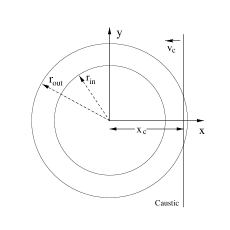
A plausible explanation of the detection of a strong iron line in image B and not in image A is the occurrence of a microlensing event in image B beginning sometime between the third and fourth observation. We estimate the size of the projected Einstein ring radius, , produced by a star of mass in the lens plane, where D represents the angular diameter distances, and the subscripts l, s, and o refer to the lens, source, and observer, respectively. For the GL system MG J0414+0534 with lens and source redshifts of and respectively, and assuming an isolated star of mass M the Einstein-ring radius on the source plane is pc. This is of the order of the line emitting region of an AGN with a black hole mass of . For our microlensing simulations we assumed a straight fold caustic traversing the accretion disk. This assumption implies that the sizes of the X-ray continuum emission and iron line reprocessing regions are much smaller than the projected Einstein radius of the perturbing star. X-ray variability studies of quasars indicate that the size of the X-ray continuum emission region is of the order of 1 10-4 pc (eg., Chartas et al. 2001). Also recent estimates (Wyithe et al. 2000; Yonehara 2001; Shalyapin, 2001) on the continuum source size in the Einstein Cross based on the analysis of a microlensing event in this system indicate that the size of the continuum emission region is less than 1 1015 cm. There are also numerous reports of similarly rapid variability in Seyfert galaxies, which place similar upper limits on the size of the X-ray source. So far, variability studies of iron lines in the spectra of radio loud quasars are scarce and the geometry of the iron line emission region in these objects is not well constrained. However, the profiles of the Fe K lines of luminous Seyfert galaxies and intermediate-luminosity quasars are quite broad and asymmetric (eg., Nandra et al. 1997), suggesting very strongly that the lines originate in the inner parts of an accretion disk where the gravitational field is quite strong. Model fits to these line profiles indicate a characteristic size of the line-emitting region of , where, , is the gravitational radius. For a 1 108 M⊙ black hole this range of sizes for the line-emitting region corresponds to 4.8 10-5 pc - 4.8 10-3 pc. We conclude that the sizes of the X-ray continuum and iron line regions in the radio-loud quasar MG J0414+0534 are likely to be smaller than the estimated projected Einstein radius, thus, making our assumption of a straight fold caustic a reasonable one. Microlensing events are produced by a star or a group of stars in the foreground lensing galaxy. Such events will not lead to time-delayed magnification in the remaining images and therefore could explain the non-detection of a strong Fe K line profile in image A during observation 5. A microlensing event could also explain the large equivalent width Fe K line (EW 910 eV) observed in image B during observation 4 and 5. As the caustic network produced by the stars in the lensing galaxy traverses the accretion disk, regions of the disk near the caustics will be magnified. For a caustic fold crossing one would expect selective magnification of a strip of the disk as shown in Figure 9, and a corresponding change in the spectrum. The magnification of a point source close to a fold caustic scales as the inverse square root of its distance to the caustic. Specifically, the amplification of a point source by a straight fold caustic is:
| (2) |
where, is the amplification outside the caustic, is the caustic amplification factor, is the coordinate perpendicular to the caustic in units of , is the position of the caustic along the x-axis and is the Heaviside function. The caustic amplification factor is of the order of , where is a constant of order unity (see equation 7 in Witt, Kayser, & Refsdal 1993). The probability distribution for K has also been computed by Wyithe & Turner (2001), who show that at optical depth of order unity the microlensing magnification patterns produced by a mass function of microlenses can be approximately reproduced by considering a mean microlens mass. We have computed the distribution of for and , appropriate for image B in the model by Ros et al. (2000), using the code of Wyithe & Turner (2001). We find that if the entire optical depth is due to stars, then the average value of is . We note that there is a factor of 2 discrepancy between the predictions of by Witt (1990) and Wyithe & Turner (2001). Given the large uncertainties, we will scale our results with .
A plausible model that can explain the observed amplification of only the iron line component and not the continuum X-ray emission places the caustic at the time of the observed amplification within the iron line emission region. To explain the non-amplification of the continuum emission during observations 4 and 5 we postulate that the thermal emission region of the disk and the Compton up-scattered emission region of the hard X-ray source lie within smaller radii than the iron line reprocessing region.
To assess the plausibility of the above hypothesis, we estimate the magnification due to the caustic crossing needed to produce the factor of 4.7 2.3 (1 errors) increase in the equivalent width of the Fe K line. For the purpose of carrying out this rough estimate, we adopt the simple disk geometry shown in Figure 9. We assume that the line is emitted within an annulus region of the accretion disk, with a radius of and the continuum source is confined to be within and it can be either a sphere (e.g., an ADAF) or a point source at or above the center of the disk (e.g., as assumed for Seyfert galaxies). The important point here is that we take the continuum source to be smaller than the emission line source.
Figure 10 shows the amplification of the iron line region by a straight fold caustic as a function of time. For this simple case we have assumed a flat emissivity profile. As the caustic crosses one side of the ring the brightness jumps by a factor of , where, and are the iron line fluxes from the ring before and after the caustic crosses the first edge, and is the center of the annulus. The reason for this jump is that flux integrated in the y direction (parallel to the caustic) has a cusp at the edges of the ring which goes to infinity if the ring is infinitely thin. As the caustic crosses this edge, a discontinuity is created. For a ring with a finite thickness, this discontinuity becomes a smooth rise with a width equal to , where is the caustic velocity and . In Figure 10 we show the amplification of the ring emission for ratios of 0.025, 0.1, 0.5 and 1 (the last case is a uniform disk of emission). After the discontinuity, more of the ring becomes amplified, rising to a peak as the caustic crosses the other edge of the ring. In practice, the maximum amplification is given by:
| (3) |
If one assumes the change in the flux of the iron line is due to a caustic crossing the disk, then the first jump condition, assuming places an upper bound on the radius of the ring of,
| (4) |
on the outer radius of the emission region. For a typical value of and for the observed amplification of the iron line of a factor of 4.7 2.3 we find pc at the 68 confidence level.
If the observed increase in the flux of the iron line in image B is occurring during the peak of the amplification curve then the upper bound on the ring radius is,
| (5) |
The constraint on the radius of the ring for the case of maximum amplification depends on and is therefore only weakly dependent on the width of the ring. For = 0.1 the second case leads to an upper bound of the ring radius of pc at the 68 confidence level. The large equivalent width of the iron line implies a large covering factor, which may require . In this case, the maximum magnification is (Witt et al. 1993), yielding an upper limit which is twice as large as the thin annulus jump condition. With the limited sampling of the amplification curve we cannot definitively distinguish which of the two cases corresponds to the observed increase in the iron line flux of image B. However, the case of maximum amplification is expected to last for a relatively short interval ( days) whereas the 4th and 5th observations of MG J0414+0534 are separated by 80 days. We therefore suggest that the observed amplification of the Fe K line is most likely caused by the initial crossing of the ring-shaped emission region by the caustic. The non-detection of any amplification of the continuum emission in image B for observations 4 and 5 implies that the caustic during these observations had not crossed the second side of the ring. Had the caustic already crossed the center of the disk it would have magnified any emission, including the continuum emission, behind the caustic. This asymmetry in microlensing by a caustic is described by the Heaviside function in equation 2. The amplification of the iron line changed by a factor of 5 over a period of about 30 days, giving a derivative of 40 mag per year. This derivative is large enough to imply that the observed change in the EW of the Fe K image B is likely due to a high-amplification event, meaning that the Fe K region is amplified by a caustic or cusp. A limit on the source size can also be obtained by calculating the probability of such a large change in amplification in image B over a short timescale as a function of source size. Such a calculation will be presented in a future publication.
Based on our simulations of caustic crossings we also expect to detect significant distortions of the iron line due to special and general relativistic effects and Doppler effects if the iron line emission region extends below 100 . “Snapshot” spectra from detailed simulations for the case where the iron line emission region extends below 100 are shown in Figure 11. The simulation assumes a flat, face-on disk about a Schwarzchild black hole with turbulent velocity equal to one percent of the Keplerian velocity. The caustic strength used for the simulations shown in Figure 11 is . These simulations assume an emissivity profile and include relativistic and Doppler effects. Based on these iron line simulations and the observed width and energy of the iron line we place a lower bound of 100 on the distance of the caustic from the center of the disk. Assuming the fold caustic at 100 we estimate that the strength of the caustic needed to explain the observed 4.72.3 increase in the EW of the iron line is . This estimate of the caustic strength was derived assuming that the un-microlensed equivalent width of the broad line is equal to 190 eV, and that the disk covers 2 of the continuum source. This relation provides an estimate of the mass of the black hole as a function of the average mass of the lensing stars. Specifically, if we assume the average mass of the stars responsible for the microlensing event to lie between 0.1 M⊙ and 1 M⊙ we estimate the mass of the black hole in MG J0414+0534 to range between M⊙ and M⊙, respectively. If the caustic is actually at a larger radius than , then a larger amplification is required, implying a smaller mass black hole. Remarkably, this indicates that the X-ray luminosity is near Eddington if the emission is unbeamed and isotropic and if the average microlens mass is near solar.
Recently, there has been considerable interest in using the lensing effect to probe for dark matter substructure in galaxy halos (Metcalf & Madau 2001; Chiba 2001). To address the question of whether such substructure can be responsible for the observed microlensing event in image B we provide an estimate of the mass of the lensing object. Assuming the quasar is emitting isotropically with an observed unlensed luminosity lying between 1 and 0.1 times the Eddington luminosity we estimate the mass of the black hole to lie between 5.3 106 and 5.3 107 M⊙, respectively. Using the constraint, , derived from our analysis of the microlensing event in MG J0414+0534 we find that the effective mass of the perturber lies in the range of M⊙ and M⊙. We conclude that the lensing object is most likely a star or group of stars and not a dark satellite in the lens galaxy. A second argument that rules against substructures as the cause of the microlensing event is that the timescale for substructure to change the X-ray fluxes is much longer than the microlensing timescale by individual stars.
If the iron line in MG J0414+0534 is concentrated in a ring with we predict to see no GR distortion as the caustic traverses the accretion disk and only a change in the intensity of the line is expected. This picture in which the iron line region is confined to large radii is supported by the results of X-ray observations of nearby radio-loud AGNs (see Woźniak et al. 1998 and Eracleous, Sambruna, & Mushotzky 2000, and references therein). Microlensing offers an independent way of testing this scenario.
The timescale for the microlensing event in image B is of the order of , where, is the size of the lensed source region and is the velocity of the caustics in the lens plane (measured in our time frame) given by equation (B9) in Kayser, R., Refsdal, S., & Stabell, R. (1986). If we assume an observer velocity of 360 km/s (this is measured from the CMB dipole), lens and AGN velocities of 600 km/s, and sum the three-dimensional velocities in equation (B9) in RMS, we find a typical velocity of a caustic of 170 km/s and a typical timescale of the microlensing event of years.
An apparent puzzle from our present observations is the predicted frequency of a caustic crossing in MG J0414+0535 of order 60 (/170 km/s)-1 years. There are several uncertain factors in this frequency estimate of order unity, the main ones being the spacing of caustics perpendicular and parallel to the shear and the optical depth of the lens. However, there are four images in MG 0414+0535 and there are about ten lenses that have been observed in the X-ray band with Chandra, so perhaps overall the detection of a microlensing event in image B is not so surprising.
If we continue to monitor MG J0414+0534 in the following years we predict that the profile of the iron line will significantly change if the iron emission region of the radio loud quasar MG J0414+0534 extends below 100. If the iron line in MG J0414+0534 is concentrated in a ring with we expect to see no GR distortion and the EW of the line in image B should return to the un-microlensed value of 190eV.
We also predict that in the upcoming months the caustic will approach the center of the accretion disk and magnify the continuum emission region. The anticipated duration of magnification of the continuum region depends on several factors that include the present distance of the caustic from the continuum emission region, the velocity of the caustic and the size of continuum emission region. Several deeper Chandra observations of MG J0414+0534 planned for the following year will allow us to possibly observe the onset of the magnification of the continuum emission region and provide a constraint on its size.
We would like to thank Pat Broos for providing the TARA software package, Koji Mori for providing subpixel correction software and the anonymous referee for providing many useful comments and suggestions. We thank Stuart Wyithe for use of his microlensing code and Jose Muñoz for providing lensing model parameters. We acknowledge financial support by NASA grant NAS 8-38252. Support for EA was provided by the National Aeronautics and Space Administration through Chandra Postdoctoral Fellowship Award Number PF0-10013 issued by the Chandra X-ray Observatory Center, which is operated by the Smithsonian Astrophysical Observatory for and on behalf of the National Aeronautics Space Administration under contract NAS8-39073.
| TABLE 1 | |||||||
| Chandra Observations of MG J0414+0534 | |||||||
| Observation | Obsid | Exposure | Roll Angle | RA1+A2a | RBb | RCc | RBkgd |
| Date | Time | ||||||
| s | (∘) | 10-3 cnts s-1 | 10-3 cnts s-1 | 10-3 cnts s-1 | 10-6 cnts -2 s-1 | ||
| 2000-01-13 | 417 | 6578 | 293.248 | 51.4 2.8 | 13.5 1.4 | 3.0 0.7 | 4.6 0.5 |
| 2000-04-02 | 418 | 7437 | 267.869 | 48.3 2.6 | 12.9 1.3 | 7.7 1.0 | 27.2 1.2 |
| 2000-08-16 | 421 | 7251 | 102.926 | 49.0 2.6 | 14.3 1.4 | 6.1 0.9 | 3.4 0.4 |
| 2000-11-16 | 422 | 7504 | 40.134 | 55.6 2.7 | 12.9 1.3 | 7.9 1.0 | 4.0 0.5 |
| 2001-02-05 | 1628 | 9020 | 277.900 | 55.4 2.5 | 16.8 1.4 | 5.9 0.8 | 5.0 0.5 |
NOTES:
a are the detected event rates from images A1 and A2 of MG J0414+0534
extracted from circular regions centered on the mid-point between A1 and A2
with radii of 1′′. Only events with standard ASCA grades 0,2,3,4,6
and energies lying between 0.2 and 10keV were selected.
b are the detected event rates from image B of MG J0414+0534
extracted from circular regions centered on B
with radii of 1′′.
c are the detected event rates from image C of MG J0414+0534
extracted from circular regions centered on C
with radii of 1′′.
d are the detected background event rates per arcsec2 extracted
from annuli centered on MG J0414+0534 with inner and outer radii of 5′′ and 30′′ respectively.
Only events with standard ASCA grades 0,2,3,4,6 were extracted.
| TABLE 2 | ||||
| OPTICAL AND X-RAY OFFSETS OF MG J0414+0534 IMAGES | ||||
| Telescope | B | A1 | A2 | C |
| (′′), (′′) | (′′), (′′) | (′′), (′′) | (′′), (′′) | |
| HST | 0,0 | 0.600.01,-1.940.01 | 0.730.01,-1.550.01 | 1.3450.01, 1.640.01 |
| Chandra | 0,0 | 0.570.02, -1.920.02 | 0.690.02, -1.530.02 | 1.300.02, 1.630.02 |
NOTE-
a Offsets in RA and Dec with respect to image C. Relative positions taken with the
Hubble Space Telescope (HST) are from Angonin-Willaime et al. (1999).
| TABLE 3 | |||
|---|---|---|---|
| MULTI-WAVELENGTH FLUX RATIOS | |||
| OF MG J0414+0534 COMPONENTS | |||
| Waveband | A1/A2 | A/B | C/B |
| 8GHz | 1.114 0.002 | 4.882 0.004 | 0.384 0.001 |
| H band | 1.36 0.05 | 4.45 0.15 | 0.46 0.02 |
| R band | 4.00 0.06 | 2.65 0.08 | 0.52 0.04 |
| I band | 2.64 0.06 | 3.06 0.07 | 0.48 0.04 |
| 2-8keV | 1.3 0.2 | 3.75 0.20 | 0.47 0.04 |
NOTE-
8GHz flux ratios are taken from the VLA data of Katz, Moore & Hewitt (1997).
The H, R, and I band data are taken from
the CfA-Arizona Space Telescope LEns Survey (CASTLES) of gravitational lenses
website http://cfa-www.harvard.edu/glensdata/.
Error bars for the X-ray data are at the 68% confidence level.
| TABLE 4 | |||||||
| RESULTS FROM SPECTRAL FITS OF ABSORBED POWER-LAW MODELS TO THE | |||||||
| INDIVIDUAL SPECTRA OF IMAGES OF MG J0414+0534 | |||||||
| Fita | Epoch | Image | Fluxb | ||||
| cm-2 | cm-2 | erg s-1 cm-2 | |||||
| 1 | I | A + B + C | 1.89 | … | 4.50 | 4.0 | 0.7(17) |
| 2 | I | A + B + C | 1.94 | 1.02 | … | 3.9 | 0.68(17) |
| 3 | I | A | 2.12 | … | 6.74 | 2.5 | 0.47(11) |
| 4 | I | A | 2.22 | 1.57 | … | 2.4 | 0.36(11) |
| 5 | II | A + B + C | 1.58 | … | 3.17 | 5.4 | 0.99(21) |
| 6 | II | A + B + C | 1.61 | 0.71 | … | 5.3 | 0.97(21) |
| 7 | II | A | 1.43 | … | 2.25 | 4.2 | 0.75(12) |
| 8 | II | A | 1.45 | 0.50 | … | 4.1 | 0.76(12) |
| 9 | III | A + B + C | 1.68 | … | 4.09 | 5.3 | 0.75(20) |
| 10 | III | A + B + C | 1.73 | 0.90 | … | 5.2 | 0.75(20) |
| 11 | III | A | 1.66 | … | 3.92 | 3.4 | 1.08(11) |
| 12 | III | A | 1.71 | 0.87 | … | 3.2 | 1.08(11) |
| 13 | IV | A + B + C | 1.66 | … | 4.50 | 5.9 | 0.89(24) |
| 14 | IV | A + B + C | 1.71 | 1.02 | … | 5.7 | 0.85(24) |
| 15 | IV | A | 1.92 | … | 6.14 | 3.2 | 0.86(14) |
| 16 | IV | A | 2.00 | 1.42 | … | 3.2 | 0.83(14) |
| 17 | V | A + B + C | 1.74 | … | 4.98 | 5.9 | 0.80(31) |
| 18 | V | A + B + C | 1.78 | 1.11 | … | 5.8 | 0.76(31) |
| 19 | V | A | 1.66 | … | 5.14 | 4.3 | 0.85(19) |
| 20 | V | A | 1.70 | 1.14 | … | 4.2 | 0.85(19) |
| 21 | ALL | A + B + C | 1.72 | … | 4.76 | 1.22(108) | |
| 22 | ALL | A + B + C | 1.76 | 1.07 | … | 1.21(108) | |
| 23 | ALL | A | 1.71 | … | 4.77 | 0.91(74) | |
| 24 | ALL | A | 1.76 | 1.08 | … | 0.89(74) | |
| 25 | ALL | B | 1.70 | … | 3.25 | 0.74(17) | |
| 26 | ALL | B | 1.76 | 0.79 | … | 0.74(17) | |
| 27 | ALL | C | 1.63 | … | 3.9 | 0.40(6) | |
| 28 | ALL | C | 1.65 | 0.87 | … | 0.35(6) | |
NOTES-
All models include Galactic absorption due to neutral cold gas with a column density of
NH = 0.1085 1022 cm-2. All derived errors are at the 90%
confidence level. The reduced chi-squared is defined as = , where ,
the number of degrees of freedom, is given in parentheses.
a The spectral fits were performed within the energy ranges 0.4 - 6 keV
b Flux is estimated in the 2-10keV band
| TABLE 5 | |||||||||
| RESULTS OF FITS THAT INCORPORATE | |||||||||
| COMPTON REFLECTION AND/OR IRON LINE EMISSION MODELS | |||||||||
| Fit | Model | Reflection | Iron Line | ||||||
| R | Ec | Eline | EW | FWHM | Fline | ||||
| (keV) | (keV) | (eV) | (km s-1) | (erg s-1 cm-2) | |||||
| 1 | pl + line | 1.70 | 6.49 | 193 | 12000 | 4.4 10-15 | 0.89(75) | ||
| 2 | pl + line | 1.72 | 6.47 | 218 | 12000 | 7.6 10-15 | 1.22(109) | ||
| 3 | pl + line + reflection | 1.62 | 100f | 6.4f | 191 | 6.7 10-15 | 1.22 (110) | ||
| 4 | pl + line + reflection | 1.67 | 500f | 6.4f | 198 | 6.9 10-15 | 1.22 (110) | ||
NOTE-
Fit 1 is performed to the combined spectra of image A for all epochs.
Fits 2, 3, and 4 are performed to the combined spectra of all images for all epochs.
and are calculated in the quasar rest frame.
The symbol denotes that the quantity is fixed during the spectral fitting process.
All quoted errors are at the 90% confidence level.
Spectral models for fits contain Galactic absorption
fixed at NH = 0.1085 1022 cm-2
and intrinsic absorption set as a free parameter.
| TABLE 6 | |||||||||
| RESULTS OF FITS TO IMAGE B THAT INCORPORATE | |||||||||
| IRON LINE EMISSION MODELS | |||||||||
| Fit | Model | Narrow Line | Broad/Disk Line | ||||||
| Eline | EW | Eline | EW | or Inc | |||||
| (keV) | (eV) | (keV) | (keV) | (keV) | |||||
| 1 | pl | 1.70 | … | … | … | … | … | … | 1.41(26) |
| 2 | pl + 1 gline | 1.69 | 6.48 | 880 | 0.15 | … | … | … | 1.25(23) |
| 3 | pl + 2 glines | 1.99 | 6.48 | 906 | 0.15 | 9.21 | 5.50 | 1.3keV | 0.94(20) |
| 4 | pl + diskline | 1.81 | 6.46 | 786 | 0.15 | 8.84 | 3.4 | 45∘ f | 1.02(21) |
NOTE-
Fits 1,2,3 and 4 are performed on the combined spectrum
of image B for observations 4 and 5.
All quoted errors are at the 90% confidence level.
and are calculated in the quasar rest frame.
Spectral models for fits contain Galactic absorption
fixed at NH = 0.1085 1022 cm-2
and intrinsic absorption set as a free parameter.
The symbol denotes that the quantity is fixed during the spectral fitting process.
References
Agol, E. & Krolik, J. 1999, ApJ, 524, 49
Anders E. & Grevesse, N. 1989, Geochimica et Cosmochimica Acta 53, 197
Anders E. & Ebihara, M. 1982, Geochimica et Cosmochimica Acta 46, 2363
Angonin-Willaime, M. -C., Vanderriest, C., Courbin, F., Burud, I., Magain, P., and Rigaut, F. 1999, Astron. & Astrophys. 347, 434
Arnaud, K. A. 1996, ASP Conf. Ser. 101: Astronomical Data Analysis Software and Systems V, ed. G. Jacoby & J. Barnes (San Francisco: ASP), 17
Blandford, R. D., & McKee, C. F. 1982, ApJ, 255, 419
Cash, W. 1979, ApJ, 228, 939
Chartas, G., Dai, X., Gallagher, S. C., Garmire, G. P., Bautz, M. W., Schechter, P. L., & Morgan, N. D. 2001, ApJ, 558, 119
Chiba, M, 2001, ApJ, astro-ph/0109499
Corrigan, R. T., Irwin, M. J., Arnaud, J., Fahlman, G. G., Fletcher, J. M., Hewett, P. C., Hewitt, J. N., Le Fevre, O., McClure, R., Pritchet, C. J., Schneider, D. P., Turner, E. L., Webster, R. L., and Yee, H. K. C. 1991, AJ, 102, 34
Eracleous, M., Sambruna, R. M., & Mushotzky, R. F. 2000, ApJ, 537, 654
Fabian, A. C., Rees, M. J., Stella, L., & White, N. E. 1989, MNRAS, 238, 729
Falco, E. E., Lehar, J., Shapiro, I. I. 1997, AJ, 113, 540
Feldman, U. 1992, Physica Scripta 46, 202
George, I. M. & Fabian, A. C. 1991, MNRAS, 249, 352
Gould, A. & Gaudi, B. S. 1997, ApJ, 486, 687
Grieger, B., Kayser, R., & Refsdal, S. 1988, A&A, 194, 54
Grieger, B., Kayser, R., & Schramm, T. 1991, A&A, 252, 508
Halpern, J. P. 1982, PhD Thesis, Harvard University
Hewitt, J. N., Turner, E. L., Lawrence, C. R., Schneider, D. P., & Brody, J. P. 1992, AJ, 104, 968
Irwin, M. J., Webster, R. L., Hewett, P. C., Corrigan, R. T., & Jedrzejewski, R. I. 1989, AJ, 98, 1989
Iwasawa, K. & Taniguchi, Y., 1993, ApJ, 413, L15
Katz, C. A., Moore, C. B., & Hewitt, J. N. 1997, ApJ, 475, 512
Kayser, R., Refsdal, S., & Stabell, R. 1986, A&A, 166, 36
Laor, A. 1991, ApJ, 376, 90
Lawrence. C, R., Elston, R., Januzzi, B. T., & Turner, E. L. 1995, AJ, 110, 2570
Magdziarz & Zdziarski 1995, MNRAS, 273, 837
Malhotra, S., Rhoads, J. E., & Turner, E. L. 1997, MNRAS, 288, 138
Matt, G., Perola, G. C., & Piro, L. 1991, A&A, 247, 25
Metcalf, R. B. & Madau, P., 2001, ApJ, astro-ph/0108224
McLeod, B. A., Bernstein, G. M., Rieke, M. J., & Weedman, D. W. 1998, AJ, 115, 1377
Mineshige, S. & Yonehara, A. 1999, PASJ, 51, 497
Nandra, K., George, I. M., Mushotzky, R. F., Turner, T. J., & Yaqoob, T. 1997, ApJ, 477, 602
Netzer, H., & Peterson, B. M. 1997, in Astronomical Time Series, ed. D. Maoz, A. Sternberg, & E. M. Liebowitz (Dordrecht: Kluwer), 85
Ostensen, R., Refsdal, S., Stabell, R., Teuber, J., Emanuelsen, P. I., Festin, L., Florentin-Nielsen, R., Gahm, G., Gullbring, E., Grundahl, F., Hjorth, J., Jablonski, M., Jaunsen, A. O., Kaas, A. A., Karttunen, H., Kotilainen, J., Laurikainen, E., Lindgren, H., Maehoenen, P., Nilsson, K., Olofsson, G., Olsen, O., Pettersen, B. R., Piirola, V., Sorensen, A. N., Takalo, L., Thomsen, B., Valtaoja, E., Vestergaard, M., and Av Vianborg, T. 1996, A&A, 309, 59
Peterson, B. M. 1993, PASP, 105, 247
Reeves, J. N. & Turner, M. J. L. 2000, MNRAS, 316, 234
Ros, E., Guirado, J. C., Marcaide, J. M., Pérez-Torres, M. A., Falco, E. E., Muñoz, J. A., Alberdi, A., & Lara, L. 2000, A&A, 362, 845
Sambruna, R. M., Eracleous, M., & Mushotzky, R. F. 1999, ApJ, 526, 60
Schechter, P. L. & Moore, C. B. 1993, AJ, 105, 1
Schneider, P., Ehlers, J., & Falco, E. E., 1992, Gravitational Lensing (New York: Springer)
Shalyapin, V. N. 2001, Astronomy Letters, 27, 150
Tonry, J. L., & Kochanek, C. S., 1999, ApJ, 117, 2034
Trotter, C. S., Winn, J. N., & Hewitt, J. N. 2000, ApJ, 535, 671
Tsunemi, H., Mori, K., Miyata, E., Baluta, C., Burrows, D. N., Garmire, G. P., & Chartas, G. 2001, ApJ, 554, 496
Wise, M. W., Davis, J. E., Huenemoerder, Houck, J. C., Dewey, D. Flanagan, K. A., and Baluta, C. 1997, The MARX 3.0 User Guide, CXC Internal Document available at http://space.mit.edu/ASC/MARX/
Witt, H. J. 1990, A&A, 236, 311
Witt, H. J., Kayser, R. & Refsdal, S., 1993, A&A, 268, 501.
Witt, H. J., Mao, S., & Schechter, P. L. 1995, ApJ, 443, 18
Woźniak, P. R., Zdziarski, A. A., Smith, D., Madejski, G. M., & Johnson, W. N. 1998, MNRAS, 299, 449
Woźniak, P. R., Alard, C., Udalski, A., Szymański, M., Kubiak, M., Pietrzyński, G., & Zebruń, K. 2000, ApJ, 529, 88
Wyithe, J. S. B., Webster, R. L., & Turner, E. L. 2000, MNRAS, 318, 762
Wyithe, J. S. B. & Turner, E. L. 2001, MNRAS, 320, 21
Yonehara, A., Mineshige, S., Fukue, J., Umemura, M., & Turner, E. L. 1999, A&A, 343, 41
Yonehara, A. 2001, ApJ, 548, L127
Young, A. J. & Reynolds, C. S. 2000, ApJ, 529, 101