Ongoing massive star formation in the bulge of M51

Abstract

We present a study of $HST-WFPC2$ observations of the inner kpc of the interacting galaxy M51 in six bands from 2550 Å to 8140 Å. The images show an oval shaped area (which we call “bulge”) of about $11\times 16$ arcsec or $450\times 650$ pc around the nucleus that is dominated by a smooth “yellow/reddish” background population with overimposed dust lanes. These dust lanes are the inner extensions of the spiral arms. The extinction properties, derived in four fields in and outside dust lanes, is similar to the Galactic extinction law. The reddish stellar population has an intrinsic color of $(B-V)_{0}\simeq 1.0$ suggesting an age in excess of 5 Gyrs.

We found 30 bright point-like sources in the bulge of of M51 i.e. within 110 to 350 pc from the nucleus. The point sources have $21.4<V<24.3$, many of which are blue with $B-V<0$ and are bright in the UV with $19.8<m_{2550}<22.0$. These objects appear to be located in elongated “strings” which follow the general pattern of the dust lanes around the nucleus. The spectral energy distributions of the point-like sources are compared with those predicted for models of clusters or single stars. There are three reasons to conclude that most of these point sources are isolated massive stars (or very small groups of a few isolated massive stars) rather than clusters:
(a) The energy distributions of most objects are best fitted with models of single stars of $M_{V}$ between -6.1 and -9.1, temperatures between 4000 and 50000 K, and with 4.2 $<$ log $L/\mbox{$L_{\odot}$}<$ 7.2, and $12<\mbox{$M_{*}$}<200~{}\mbox{$M_{\odot}$}$.
(b) In the HR diagram the sources follow the Humphreys-Davidson luminosity upper limit for massive stars.
(c) The distribution of the sources in the HR diagram shows a gap in the range of $20~{}000<\mbox{$T_{\rm eff}$}<10~{}000$ K, which agrees with the rapid crossing of the HRD by stars, but not of clusters.
We have derived upper limits to the total mass of lower mass stars ($\mbox{$M_{*}$}<10~{}\mbox{$M_{\odot}$}$), that could be “hiding” within the point sources. For the “bluest” sources the upper limit is only a few hundred $M_{\odot}$.

We conclude that the formation of massive stars outside clusters (or in very low mass clusters) is occurring in the bulge of M51.

The estimated star formation rate in the bulge of M51 is 1 to $2\times 10^{-3}$ $M_{\odot}~{}yr^{-1}$, depending on the adopted IMF. With the observed total amount of gas in the bulge, $\sim 4\times 10^{5}$ $M_{\odot}$, and the observed normal gas to dust ratio of $\sim 150$, this star formation rate could be sustained for about 2 to $4\times 10^{8}$ years. This suggests that the ongoing massive star formation in the bulge of M51 is fed/triggered by the interaction with its companion about $4\times 10^{8}$ years ago. The star formation in the bulge of M51 ia compared with tat in bulges of other spirals.

Theoretical predictions of star formation suggest that isolated massive stars might be formed in clouds in which H₂, [OI] 63 $\mu$m and [CII] 158 $\mu$m are the dominant coolants. This is expected to occur in regions of rather low optical depth, $A_{V}\leq 1$, with a hot source that can dissociate the CO molecules. These conditions are met in the bulge of M51, where the extinction is low and where CO can be destroyed by the radiation from the bright nuclear starburst cluster in the center. The mode of formation of massive stars in the bulge of M51 may resemble the star formation in the early Universe, when the CO and dust contents were low due to the low metallicity.

1 Introduction

The spiral galaxy M51 (NGC 5194, the Whirlpool nebula) and its peculiar companion galaxy NGC 5195 form a typical example of galaxy interactions. After the pioneering hydrodynamical simulations by Toomre and Toomre (1972), several authors have tried to explain the grand design spiral shape and the tidal arms of this interacting system. Hernquist (1990) and Barnes (1998) have critically discussed the successes and the problems of explaining the morphology of the NGC 5194/5195 system, in particular the radial velocities of the two galaxies, the two-armed spiral structure of M51, the connecting tidal arm and the large H i arm. The best model is found for a relative orbit that is almost in the plane of M51, for a mass ratio of NGC 5194/5195 $\simeq 2$, a pericenter distance of 17 to 20 kpc and a time since pericenter of $2.5\times 10^{8}<t<4\times 10^{8}$ yrs (Barnes 1998).

The NGC 5194/5195 system is ideally suited for the study of triggered star formation due to galaxy-galaxy interactions. For this reason we have started a series of studies on the different aspects of star formation in M51, based on $HST-WFPC2$ observations in six broadband filters. The nucleus was studied by Scuderi et al. (2001; hereafter called Paper I), who found that it contains a total stellar mass of about $2\times 10^{7}$ $M_{\odot}$ within the central 17 pc and a bright point source of $2\times 10^{6}$ $M_{\odot}$ within the inner 2 pc. In this paper we study the properties of the elongated “yellow/reddish” region around the nucleus, hereafter called “the bulge”, and of 30 bright point-like sources that we discovered in it. These point sources indicate ongoing star formation in the bulge region, which is otherwise dominated by old ($>$ 5 Gyrs) stars (Paper I).

The full $HST-WFPC2$ image of M51 is published is Paper I. The image shows that the nucleus is surrounded by an elongated bulge of about 460 $\times$ 860 pc that is dominated by an old stellar population. The spiral arms containing H II regions start outside the bulge. We adopt a distance of $d=8.4\pm 0.6$ kpc, corresponding to a distance modulus of $29.62\pm 0.16$, which is based on the brightness distribution of planetary nebulae (Feldmeier, Ciardullo & Jacoby 1997). At this distance, 1 arcsec corresponds to a linear distance of 40.7 pc, one $HST-PC$ pixel of 0.046^" corresponds to 1.87 pc and an $HST-WFC$ pixel of 0.1^" corresponds to 4.1 pc.

In § 2 we describe the observations and the data reduction. In § 3 we discuss the interstellar extinction in the bulge. In § 4 we describe the properties of 30 bright point-like sources in this region. In § 5 their energy distributions are compared with those predicted for clusters with different ages and mass, and for single stars of different effective temperatures and radii. We will show that most of them are very luminous young stars (single or multiple), rather than clusters. The star formation rate in the bulge of M51 is derived in § 6. In § 7 we compare the formation of massive stars in the bulge of M51 with clusters near the Galactic center, in the interaction region of the Antennae galaxies, and in the bulges of other spiral galaxies. We also discuss the predicted mode of star formation under the conditions that prevail near the nucleus of M51. The conclusions are given in § 8.

2 Observations and Data Reduction

M51 was observed with $HST-WFPC2$ on May 12, 1994 and on January 15, 1995 as part of the $HST$ Supernova Intensive Study (SINS) program to study SN 1994I (e.g., Millard et al. 1999). The galaxy was observed through the wide band filters F255W and F336W in 1994 and through the wide band filters F439W, F555W, F675W and F814W in 1995. We will refer to these filters as the $UV$, $U$, $B$, $V$, $R$, and $I$ filters. The observations in the $UV$, $U$ and $B$ filters were split into four, three and two exposures of 500, 400, 700 $s$ respectively, while a single exposure of 600 $s$ was taken with the remaining filters.

The data were processed through the PODPS (Post Observation Data Processing System) pipeline for bias removal and flat fielding. The removal of the cosmic rays in the $UV$, $U$ and $B$ images was accomplished by combining the available exposures. For the images taken in the other three filters we used a simple procedure, which consists in combining images obtained in adjacent bands, that allowed us to remove most of the contribution from the cosmic rays (see Paper 1). Unfortunately the corrected images still showed some residual contamination from cosmic rays which could have affected the photometry. To obtain a list of the point-like sources in each filter we used an unsharp masking method. This was done because of the complexity of the background emission. In fact, it seems that most of the point-like sources lie on or close to dust lanes that are the inner extensions of the spiral arms structures. The method consisted in smoothing each image using a Gaussian with 4 pixels FWHM and then subtracting the smoothed image from the original image. From each image the list of sources was obtained by picking up all the objects above a threshold, variable from about 3 to 13 times the local value of the background depending on the filter. These lists contained also residual cosmic rays so we “cross–correlated” them, selecting only those objects that were present in at least two different filters.

This procedure was applied only to the optical filters. The $UV$ and $U$ images were taken 8 months earlier than the optical images, which means that the orientation of the spacecraft was not the same in the two epochs. In the 1995 observations the nucleus of M51 was near the center of the PC-images, but in 1994 the images were centered on SN 1994I and the nucleus was at the edge of the PC-image. This means that the $UV$ and $U$ observations of about half of the point sources were made with the PC-camera and the rest were made with the WF-camera.

To obtain the photometry of the point-like sources in the $UV$ and $U$ filters we first took the list containing the positions (pixel coordinates) of the point-like sources in the optical images and rotated the image, taking the position of SN 1994I as origin, to match the different orientation. In this way we identified the same point-like sources in the $UV$ images as in the optical images.

We performed aperture photometry using an aperture radius of 2 pixels and calculating the sky background in an annulus with internal and external radius of 5 and 8 pixels respectively. The correction for the aperture was obtained from a theoretical PSF obtained with Tiny Tim (Krist & Burrows 1994). The flux calibration was obtained using the internal calibration of the $WFPC2$, using the spectrum of Vega as photometric zero-point (Whitmore 1995). The uncertainty in the photometry was computed by taking into account photon noise, background noise and CCD read-out noise only. Charge transfer and distortion effects were not taken into account. Tests showed that these effects have little influence on the colours (less than about 0.03 magn) and on the magnitudes (less than 0.04 magn).

Figure 1 shows the $B$-image taken with the Planetary Camera. The bulge region is indicated. Figure 2 shows the region of the bulge enlarged. The symbols and the marked areas are described below.

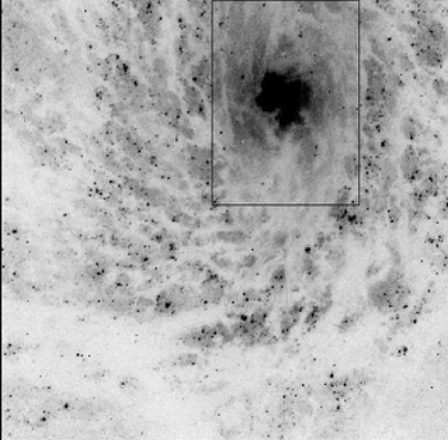
Figure 1: The negative $F439W$ image of M51 taken with the $HST$ Planetary Camera. The field is $36.8\times 36.7$ arcsec or $1.48\times 1.48$ kpc. The nucleus and the spiral arms are clearly visible. The rectangle indicates the “bulge region” that is enlarged in Figure 2. The dust lanes in the bulge follow a spiral structure as if they are the inner extensions of the spiral arms seen at larger distance.

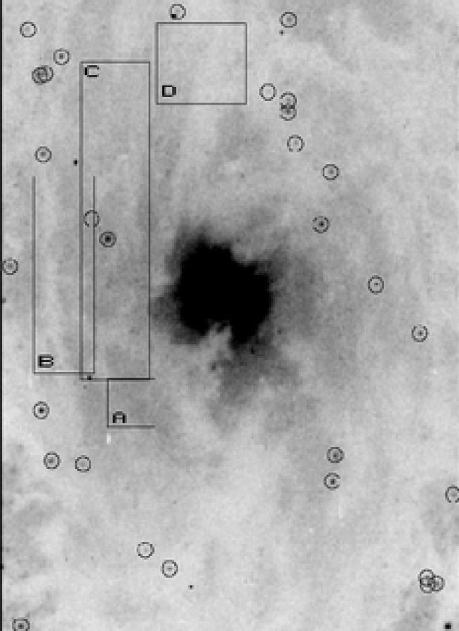
Figure 2: The negative $F439W$ image of the region of $11\times 16$ arcsec or $450\times 650$ pc around the nucleus of M51 observed with the $HST-PC$-camera. Apart from the nucleus and the dust lanes, the region has a smooth structure with colors indicating an old, $>5\times 10^{9}$ yrs, population. The four fields, used for studying the extinction curve and the location of the “bulge point sources” are indicated.

3 The interstellar extinction

The region around the nucleus of M51, in an area of about 11 $\times$ 16 arcsec = 460 $\times$ 680 pc, appears “yellow/reddish” in the $HST$ images. The light from this region, the bulge, is dominated by an old stellar population. The brightness distribution in the bulge is smooth and homogeneous in color apart from the many darker “lanes” which are obviously due to dust extinction, see Fig. 2. Assuming a homogeneous stellar distribution in color and magnitudes, the extinction can be studied by comparing the magnitudes and colors of the dusty regions with those in adjacent regions were the extinction appears to be small.

To this purpose we have selected in the bulge four areas with different extinctions (Fields A to D). The locations of these fields are indicated in Fig. 2. For each of the fields we constructed $m_{\lambda}$ versus $V$ and color-color plots of all the pixels. Figure 3 shows the $m_{\lambda}$ versus $V$ plots for fields A and C. Assuming that the background population of bulge stars has a uniform colour (see Paper I), the slopes of the relations give the extinction ratios. The range of the magnitudes in each field provide an estimate of the maximum extinction values. We find that the extinction in the bulge is small and has a maximim value of about 0.25 in $E(B-V)$, in agreement with Paper I.

The resulting values of the extinction ratios are listed in Table 1 where the values are also compared with the Galactic values for the same $HST$ filters based on the extinction curve of Savage and Mathis (1979). The Galactic values were derived by applying the extinction curve to the stellar energy distribution of an unreddened A0-star and then convolving the resulting spectrum with the $HST$ filter characteristics (for details, see Romaniello 1998, and Romaniello et al. 2001). The table shows that the extinction ratios are quite similar to those of our Galaxy, which suggests that the extinction curve of the two galaxies are about the same. Scuderi et al. (2001) have reached the same conclusion for the M51 nuclear region, but using a somewhat different method.

Hill et al. (1997) have shown on the basis of a study of HII regions observed with the Ultraviolet Imaging Telescope that the far-UV extinction of M51 is smaller than in the Galaxy, $A_{152}/E(B-V)=6.80$ for M51 compared to 8.33 for the Galaxy. This is not in contradiction with our results, because the far-UV extinction at $\lambda<2100\AA$ is known to vary drastically both in the Galaxy and in the LMC between different regions.

Figure 3: The $m_{\lambda}$ versus $V$ plots (in the Vega-magnitude sytem) for the $B$, $R$ and $I$ bands of the fields A (left) and C (right) of the bulge used for the study of the extinction law in the bulge. The slope of these relations define the extinction ratios $A_{\lambda}/A_{V}$.

Table 1: Reddening in the Galaxy and in the bulge of M51

Ratio	Galaxy	M51
$E(B-I)/E(B-V)$	2.22	$2.14\pm 0.25$
$E(V-I)/E(B-V)$	1.52	$1.15\pm 0.25$
$E(R-I)/E(B-V)$	0.66	$0.37\pm 0.15$
$A_{UV}/E(B-V)$	6.71
$A_{U}/E(B-V)$	5.04
$A_{B}/E(B-V)$	4.17
$A_{V}/E(B-V)$	3.26
$A_{R}/E(B-V)$	2.46
$A_{I}/E(B-V)$	1.90

In the above described analysis we have treated the extinction as a foreground effect. This is justified by the small values of $E(B-V)<0.25$, for which the effect of the extinction on the flux is independent of the depth distribution of the dust. The fact that we find an extinction curve closely resembling the Galactic one provides additional support to the justification of the adopted method.

4 Bright point sources in the bulge

The $HST-PC$ image of the central region of M51 (see Fig. 2) shows the presence of bright pixel-size spots, with $21.4<V<24.4$. We have estimated the sizes of the sources, using radial profile fitting using radial profile fitting of the F555W images. The vast majority, 21 out of 30, are definitely point sources. Six sources have a too high background to allow a reliable size determination. All of them are rather blue with $B-V<0.32$ (see below). Two sources (nrs 11 and 13) are possibly extended, but they have a low peak countrate and are rather faint. One of these, nr 11, is a very red source with $B-V=1.8$ whereas nr 13 is a blue source with $B-V=-0.09$ (see below). Only one source, nr 4 with $B-V=0.90$ is definitely resolved. If its intrinsic intensity distribution is Gaussian, it has an intrinsic FWHM of 0.06 arcsec, which corresponds to 2.4 pc at the distance of M51. Assuming that the sample of sources that have no reliable FWHM determination contains the same fraction of extended sources as the rest, we conclude that our sample may contain no more than 4 extended sources. From here-on the sources will be called “bulge point sources”.

Could the bulge point sources be back-ground galaxies? Using the number and magnitude distribution of galaxies in the Hubble Deep Field (Williams et al. 1996), Gonzalez et al. (1998) derived the expected number and brightness distribution of background galaxies in the $HST-WF$ chips of an observation similar to the ones of M51. Our detection limit is about 23.5 magn in $V$ and $I$, due to the bright background by the old stellar background population in the bulge. From the study of Gonzalez et al. (1998) we find that about 13 background galaxies in $V$ and 25 in $I$ above the detection limit are expected in the three $WF$-chips together. The bulge of M51 covers an area wchich is only 17 % of the $PC$-chip and 1.5 % of the three $WF$-chips together. So we expect that the bulge image contains about 0.2 background galaxies in $V$ and 0.3 in $I$. Moreover background galaxies would not be point sources. Even the extended source nr 4, with its FWHM of 0.6 arsec, is too small to be a background galaxy (unless it is a QSO). It is most likely a small cluster.

4.1 The location of the bulge point sources

The location of the bulge point sources is indicated in Fig. 2. The points are not randomly distributed, but seem to be located preferentially in an ellipse (with major axis running from upper left to lower right) or in strings around the nucleus. This agrees with the general appearance of the region around the nucleus as observed in the $B$ filter: the darker lanes also indicate spiral arms which can be traced down to the nucleus. The main spiral arms originate at a larger distance $\sim 13^{\prime\prime}\sim 500$ pc from the nucleus, i.e. just outside the range of Fig 2 (see Figure 1).

Figure 4 shows the locations and the numberings of the point sources. From the originally selected 33 sources, 3 have been removed because we could not derive reliable photometry. These are indicated by the number zero. The numbers of the remaining 30 other sources are indicated. The coordinates of the sources are listed in Table 2..

Figure 4: The location and the numbers of the 30 point sources in the Bulge of M51, that are studied in this paper. Sources with number zero were in the original selection (see Figure 2) but were not studied because of the lack of reliable photometry. The cross indicates the location of the nucleus of M51 (Paper I). The orientation is the same as in Fig. 2

4.2 Photometry of the bulge point sources

The integrated fluxes of the point sources were measured in the $UV$, $U$, $B$, $V$, $R$ and $I$ bands, as described in Sect. 2, and converted into Vega-magnitudes, where $UV=U=B=V=R=I=0$ for Vega (Whitmore 1995). Fourteen out of the 30 point sources could not be measured in the $UV$ and $U$ band because they are too faint. For these point sources we adopted safe brightness upper limits of $UV=21.4$ and $U=22.3$, which correspond to the magnitudes (minus its uncertainty) of the faintest point sources that were detected in the $UV$ and $U$ band images. Sources nr 26 and 27, which are located close together, could not be measured separately in the $UV$ and $U$ images of the WF-chips. We measured the combined magnitudes of the two sources: $UV=19.79\pm 0.11$ and $U=20.51\pm 0.06$. These two sources are resolved in the other bands, where they are in the PC-chip. Since the energy distributions of the two sources in the $B,V,R,I$ bands are very similar with a mean magnitude difference of 0.30, we adopt the same difference for the $UV$ and $U$ magnitudes, and derived the magnitudes of the two individual sources. The magnitudes of all bulge point sources are listed in Table 2.

Most sources have $B-V$ colors between $-0.5$ and $+1.0$ with two red exceptions near $B-V\simeq+2.0$ (nrs 3 and 11) and one very uncertain blue exception, namely nr 16 with $B-V=-2.5$. Most sources with $B-V<+0.5$ are detected in the $UV$ and $U$ band. The three bluest UV sources are nrs 12, 26 and 27 which have $-2.1<U-V<-1.7$ and $-3.1<UV-V<-2.6$. These must be hot objects with little or no extinction. The colors of the majority of the point sources, in the range of $-0.3\leq B-V\leq+1.0$, correspond to spectral types between O and G5, if there were no extinction. The reddest point sources, nrs 3 and 11, have $B-V=+2.2$ and +1.8 respectively, which correspond to unreddened M stars.

Table 2: Bulge point sources as clusters or stars

		CLUSTERS				STARS
Nr	nr obs	$E(B-V)$	log($t$)	log($M_{i}$)a	$\chi_{R}^{2}$	$E(B-V)$	log $T_{\rm eff}$	log $L_{*}$	$\chi_{R}^{2}$
		magn	yrs	$M_{\odot}$		magn	K	$L_{\odot}$
1	6	0.20	5.35${}_{-0.05}^{+0.80}$	3.27	3.45	0.64	4.70${}_{-0.22}^{+0.00}$	7.31${}_{-0.68}^{+0.03}$	0.52
2	4	0.18	5.35${}_{-0.00}^{+1.30}$	2.72	0.30	0.36	4.34${}_{-0.44}^{+0.00}$	5.70${}_{-0.58}^{+0.00}$	0.12
3	4	0.70	9.70${}_{-0.80}^{+0.00}$	5.63F	0.90	0.50	3.65${}_{-0.00}^{+0.00}$	5.23${}_{-0.04}^{+0.02}$	0.10
4	4	0.48	8.70${}_{-0.22}^{+0.08}$	5.28F	0.39	0.70	3.85${}_{-0.00}^{+0.27}$	5.96${}_{-0.00}^{+0.75}$	0.12
5	6	0.00	8.90${}_{-0.06}^{+0.00}$	4.85F	14.47	0.02	3.78${}_{-0.00}^{+0.00}$	5.18${}_{-0.02}^{+0.07}$	9.09
6	6	0.00	6.20${}_{-0.00}^{+0.00}$	2.46	2.18	0.10	4.48${}_{-0.10}^{+0.18}$	5.66${}_{-0.32}^{+0.57}$	0.13
7	4	0.00	8.74${}_{-0.09}^{+0.00}$	4.43F	0.03	0.24	3.85${}_{-0.00}^{+0.27}$	5.10${}_{-0.02}^{+0.76}$	0.12
8	6	0.12	6.60${}_{-0.00}^{+0.00}$	2.72	0.40	0.38	4.60${}_{-0.26}^{+0.10}$	6.58${}_{-0.76}^{+0.40}$	0.88
9	4	0.00	9.18${}_{-0.18}^{+0.00}$	4.48F	0.08	0.24	3.78${}_{-0.04}^{+0.60}$	4.84${}_{-0.22}^{+1.82}$	0.18
10	6	0.18	6.45${}_{-0.10}^{+0.00}$	2.79	0.70	0.24	4.30${}_{-0.00}^{+0.02}$	5.75${}_{-0.03}^{+0.07}$	0.10
11	4	0.46	9.65${}_{-1.48}^{+0.00}$	5.08F	1.40	1.32	3.90${}_{-0.33}^{+0.80}$	5.87${}_{-1.07}^{+2.30}$	1.10
12	6	0.00	5.60${}_{-0.00}^{+0.25}$	2.64	12.49	0.00	4.70${}_{-0.00}^{+0.00}$	6.17${}_{-0.00}^{+0.13}$	3.12
13	4	0.02	7.25${}_{-0.00}^{+0.05}$	2.82	3.23	0.18	3.88${}_{-0.03}^{+0.10}$	4.59${}_{-0.21}^{+0.33}$	30.18
14	6	0.28	6.20${}_{-0.85}^{+0.20}$	2.88	1.58	0.54	4.70${}_{-0.22}^{+0.05}$	6.65${}_{-0.66}^{+0.20}$	0.51
15	6	0.02	6.65${}_{-0.20}^{+0.00}$	2.76	5.00	0.34	4.30${}_{-0.15}^{+0.40}$	5.93${}_{-0.52}^{+1.15}$	3.19
16	3
17	4	0.00	7.00${}_{-0.00}^{+0.00}$	2.71F	6.15	0.00	4.36${}_{-0.00}^{+0.24}$	4.96${}_{-0.00}^{+0.89}$	0.61
18	6	0.22	5.30${}_{-0.30}^{+0.30}$	2.89	0.32	0.52	4.70${}_{-0.30}^{+0.00}$	6.90${}_{-0.90}^{+0.05}$	0.41
19	4	0.20	7.48${}_{-0.00}^{+1.34}$	3.65F	18.73	0.14	3.81${}_{-0.00}^{+0.00}$	4.88${}_{-0.05}^{+0.05}$	20.54
20	4	0.00	8.85${}_{-0.37}^{+0.00}$	3.88F	5.63	0.00	3.78${}_{-0.00}^{+0.00}$	4.22${}_{-0.00}^{+0.10}$	4.28
21	6	0.18	9.18${}_{-0.36}^{+0.37}$	5.22F	2.86	1.22	4.65${}_{-0.27}^{+0.05}$	8.17${}_{-0.77}^{+0.16}$	0.63
22	6	0.20	6.45${}_{-0.00}^{+0.00}$	2.79	1.89	0.30	4.38${}_{-0.23}^{+0.27}$	5.97${}_{-0.70}^{+0.86}$	1.76
23	4	0.20	6.50${}_{-0.00}^{+0.00}$	2.95	0.17	0.20	3.88${}_{-0.03}^{+0.24}$	4.86${}_{-0.14}^{+0.66}$	0.44
24	6	0.02	6.20${}_{-0.05}^{+0.00}$	2.43	1.47	0.14	4.48${}_{-0.13}^{+0.22}$	5.66${}_{-0.48}^{+0.73}$	0.57
25	4	0.00	7.54${}_{-0.00}^{+0.00}$	3.25F	11.83	0.06	4.00${}_{-0.05}^{+0.00}$	4.69${}_{-0.14}^{+0.03}$	1.21
26	6	0.00	6.35${}_{-0.00}^{+0.05}$	2.58	2.48	0.00	4.36${}_{-0.00}^{+0.34}$	5.49${}_{-0.00}^{+1.06}$	0.77
27	6	0.00	6.40${}_{-0.00}^{+0.00}$	2.42	1.98	0.00	4.36${}_{-0.00}^{+0.24}$	5.36${}_{-0.00}^{+0.76}$	0.99
28	4	0.02	9.40${}_{-0.22}^{+0.00}$	4.69F	0.09	0.34	3.78${}_{-0.00}^{+0.00}$	4.97${}_{-0.00}^{+0.00}$	0.03
29	6	0.00	5.50${}_{-0.00}^{+0.00}$	2.42	2.71	0.26	4.70${}_{-0.30}^{+0.00}$	6.36${}_{-0.98}^{+0.17}$	1.49
30	4	0.22	6.20${}_{-0.55}^{+0.20}$	2.55	0.05	0.22	4.00${}_{-0.12}^{+0.30}$	4.65${}_{-0.33}^{+0.85}$	0.02

^a: $M_{i}$ is the initial mass of the clusters.
^F: Frascati cluster model was adopted.

5 Modelling the energy distribution of the bulge point sources

The bulge point sources have visual magnitudes between 21.4 and 24.4 corresponding to $-8.2<M_{V}<-5.2$ if there were no extinction. For a mean reddening of $E(B-V)\simeq 0.3$ (see below) the absolute magnitudes are about $-9.1\leq M_{V}\leq-6.1$. This means that the bulge point sources could be either small clusters or very bright stars. We will consider both possibilities.

5.1 Bulge point sources as clusters

If the blue point sources are clusters, they cannot be very massive. For instance a cluster with an initial mass of $10^{6}$ $M_{\odot}$  and an age of $2\times 10^{6}$ years will have a visual absolute magnitude of $M_{V}=-15.3$ (Leitherer & Heckman, 1995). At the distance of M51 and with an extinction of $E(B-V)=0.3$ the cluster will have $V\simeq 15.3$. The observed point sources are 7 to 9 magnitudes fainter, so their initial mass must have been a few $10^{2}$ to a few $10^{3}$ $M_{\odot}$. For clusters of such a small mass, the colors and magnitudes cannot be accurately predicted because they will depend on the evolutionary stage of one or few of the most luminous and most massive stars. Therefore, the results of fitting the observed energy distributions to models should only be considered as a rough estimate of the cluster parameters.

We have fitted the observed energy distributions of the bulge point sources with those predicted for instantaneously formed clusters, from Leitherer & Heckman (1995), henceforth called “LH-models” and from the Frascati-group (see below), henceforth called the “Frascati-models”.

We adopted the LH-models of clusters with solar metallicity, with an IMF of $\alpha=2.35$ (Salpeter’s value) and with an upper mass cut-off of 100 $M_{\odot}$ and a lower mass cut-off of 1 $M_{\odot}$. These models cover an age range from 0.2 to 300 Myrs. The predicted magnitude in the $F255W$ band was derived from their magnitude at 2100 Å and the slope of the spectral energy distribution between 2100 and 3000 Å. The ”Frascati-models” were calculated by Romaniello (1997) from the evolutionary tracks of Brocato & Castellani (1993) and Cassisi et al. (1994) using the WFPC2 magnitudes derived from the stellar atmosphere models by Kurucz (1993). These models are for instantaneous formation of a cluster of solar metallicity stars in the mass range of 0.6 to 25 $M_{\odot}$, distributed according to Salpeter’s IMF. These models cover an age range of 10 to 5000 Myr. The LH-models are expected to more accurate for the younger clusters, because they are based on the evolutionary tracks of the Geneva-group which include massive stars. The Frascati models are expected to be more accurate for the old clusters, because they include stars with masses down to 0.6 $M_{\odot}$. For both sets of cluster-models the magnitudes were calculated directly from the predicted energy distributions, using the $WFPC2$ filter calibration (Whitmore 1995). These magnitudes will be compared directly with the observed magnitudes, so we do not have to apply the “Holtzman et al.” (1995) colour correction, which is needed when the magnitudes of the models are given in the standard filters.

For fitting the predicted to the observed energy distributions we used a three dimensional maximum likelyhood method. The free parameters are $E(B-V)$, the initial mass, $M_{i}$, and age, $t$. We corrected the observed magnitudes for extinction in the range of $0.00<E(B-V)<2.0$ in steps of 0.02. The extinction values listed in Table 1 were adopted. The weighting factors are chosen as $w_{i}=1/(\Delta m_{i})^{2}$ where $\Delta m_{i}$ is the uncertainty in the magnitude. For sources that were not detected in the $UV$ and $U$ images we adopted brightness upper limits of $UV>21.4$ and $U>22.3$, as discussed above. The uncertainty in the fitting of the $UV$ and $U$ magnitudes to the models depends more strongly on the accuracy of the adopted extinction curve than on the accuracy of the observed magnitudes. This uncertainty of the short wavelength fitting will be larger for objects with large values of $E(B-V)$. To take this into account we have added an extra term in the uncertainty of $\Delta UV=1.5~{}E(B-V)$ and $\Delta U=1.0~{}E(B-V)$ in the model fitting of the $UV$ and $U$ magnitudes, with a minimum uncertainty of $(\Delta UV)_{\rm min}=0.15$ and $(\Delta U)_{\rm min}=0.10$. This implies that the fitting had be done in two steps: first with the normal values of $\Delta m_{i}$ to find the best fit of the cluster parameters and $E(B-V)$ and then with the extra uncertainty in the $UV$ and $U$ magnitudes. The values of $E(B-V)$ of the second iteration turn out to be very similar to those of the first iteration.

The resulting fits of the LH-models and the Frascati-models were compared and one of the two was adopted, based on the following criteria: (a) significantly smaller reduced $\chi_{R}^{2}$; (b) significantly smaller value of $E(B-V)$. This last criterium is used because all reliable fits (small $\chi_{R}^{2}$) have a small extinction and because the study of the extinction (see §3) showed that $E(B-V)$ is very small in the bulge. So if the energy distribution can be fitted with a young cluster of high extinction or an older cluster of low extinction, we adopted the second solution. The uncertainties in the ages and initial masses are derived from the requirement that only fits with $\chi_{R}^{2}<\chi_{R}^{2}(min)+1$ are acceptable. This corresponds to the 68 % confidence range.

Figure 5: A comparison between the observed magnitudes of the bulge point sources (circles with errorbars) and the fits of cluster models (upper figure) and stellar models (lower figure) with extinction. In the upper figure the full lines indicate Leitherer & Heckman (1995) models and dashed lines indicate “Frascati-models”. Arrows indicate upper limits. The vertical scale is $m_{\lambda}-V$ in magnitudes and the horizontal scale is $\lambda(\AA)/1000$. In the upper figure the fits to LH-models are indicated by full lines, those of the Frascati models with dashed lines. The fit parameters are listed in Table 3.

The results are listed in the left half of Table 2 and the fits are shown in Figure 5a. For most sources a fit with a reasonably small value of $\chi_{R}^{2}\lesssim 3$ is found, however 7 sources have a high value of $\chi_{R}^{2}>5$. The cluster parameters of these models are not reliable. The results in Table 2 confirm our previous estimate that the young clusters have a low mass. More than half of the clusters have an initial mass smaller than about 1000 $M_{\odot}$. Only old clusters with $t>500$ Myrs have $M_{i}>10^{4}$ $M_{\odot}$. This is due to the detection limit. A cluster with an initial mass is below $5\times 10^{3}$ $M_{\odot}$ fades below the detection limit at an age of about 300 Myrs (Leitherer & Heckmann, 1995).

5.2 Bulge point sources as individual stars

We have also fitted the energy distributions of the bulge point sources to those predicted by model atmospheres of Kurucz (1993). For this purpose we selected 15 models with temperatures ranging from 3750 K to 50000 K and the lowest gravities in the grid of model atmospheres. We realize that the Kurucz blanketed LTE-model atmospheres may not be very accurate for the hottest stars where Non-LTE effects and atmospheric extension effects may play a role. So these models are not expected to give accurate values of the stellar parameters based on $WFPC2$-photometry. However, they serve the present purpose of obtaining an indication of the effective temperature and luminosity of the bulge point sources.

The models were fitted to the observations using a three dimensional maximum likelyhood method. The free parameters are $E(B-V)$, $T_{\rm eff}$ and radius $R_{*}$. To fit the observed energy distributions to those of model atmospheres, we corrected the observed magnitudes for extinction in the range of $0.00<E(B-V)<2.0$ in steps of 0.02 (similar to the fit of the cluster models). The resulting dereddened energy distributions were compared to those of the model atmospheres and the best-fit model was determined. The two fit parameters for the shape of the energy distributions are $E(B-V)$, $T_{\rm eff}$. The fit parameter for the absolute magnitude is the angular diameter or radius of the star. The weights of the fitting are the same as described in the previous section. To take into account the uncertainty in the extinction at the wavelengths of the $UV$ and $U$ filter, we have added an extra uncertainty $\Delta UV$ and $\Delta U$, as described in the previous section.

The results are listed in the right hand side of Table 2. We list the values of $E(B-V)$, $T_{\rm eff}$ and log $L/L_{\odot}$ and the value of the reduced $\chi_{R}^{2}$ of the fit. The range of acceptable parameters was determined in the same way as for clusters, i.e. the acceptable models have $\chi_{R}^{2}<\chi_{R}^{2}(min)+1$. Notice that for almost all sources which are observed in six wavelength bands, the fits of the energy distributions to stellar models are significantly better (smaller $\chi_{R}^{2}$) than fits to the cluster models. In total 23 objects have $\chi_{R}^{2}<3$ and only 3 have $\chi_{R}^{2}>5$.

The values of $E(B-V)$ derived from the fits are in the range of 0.0 to 1.3, with more than half of the objects having $E(B-V)<0.30$. The uncertainty in the derived values of $E(B-V)$ affects the uncertainty in $T_{\rm eff}$ and log $L$. A higher value of $E(B-V)$ corresponds to a higher value of $T_{\rm eff}$, a higher value of $L_{*}$  (because the bolometric correction increases with $T_{\rm eff}$) and a smaller radius of the object. We list the uncertainty in log $T_{\rm eff}$ and log $L_{*}$, but not in $E(B-V)$. The uncertainty in log $L_{*}$ is related to the uncertainty in log $T_{\rm eff}$ by $\Delta{\rm log}L_{*}\simeq 6.7\times\Delta{\rm log}\mbox{$T_{\rm eff}$}$ for the hottest stars with $\mbox{$T_{\rm eff}$}>30~{}000$ K and $\Delta{\rm log}L_{*}\simeq 5.3\times\Delta{\rm log}\mbox{$T_{\rm eff}$}$ for the stars with $10~{}000<\mbox{$T_{\rm eff}$}<30~{}000$ K. For stars in the range of $5000<\mbox{$T_{\rm eff}$}<10~{}000$ K, the BC is very small and almost independent of $T_{\rm eff}$. For the coolest point source in our sample, i.e. nr 3, the BC is sensitive to $T_{\rm eff}$ but the uncertainty in the derived value of $T_{\rm eff}$ is very small. Typical uncertainties are $\Delta E(B-V)\simeq 0.10$, $\Delta$ log $T_{\rm eff}$$\simeq$ 0.1 and $\Delta$ log $L_{*}$$\simeq$ 0.4 for hot stars observed in all six bands, and $\Delta E(B-V)\simeq 0.20$, $\Delta$ log $T_{\rm eff}$$\simeq$ 0.2 and $\Delta$ log $L_{*}$$\simeq$ 0.6 for the cooler stars observed in the visual colors only. For stars with $\mbox{$T_{\rm eff}$}>30~{}000$ K the uncertainty is larger (possibly as large as 10 000 K at $\mbox{$T_{\rm eff}$}>40~{}000$) due to the uncertainties in the adopted Kurucz (1993) model atmospheres.

Figure 5b shows the comparison between the observed magnitudes and the predicted magnitudes of the best fit model for each point source as a function of wavelength. The observed lower limits are also indicated. Notice that the agreement is satisfactory for almost all models. We discuss some typical energy distributions.
– Source 3 is the reddest object in our sample. It fits the energy distribution of a cool star of $T_{\rm eff}$= 4500 K with a large extinction of $E(B-V)=0.50$.
– Sources 12, 26 and 27 are the three objects with the brightest relative $UV$ magnitude in our sample. They have an energy distribution of a hot star of $T_{\rm eff}$= 50 000 K (nr 12) or 23 000 K (nrs 26 and 27) without extinction.
– Source 20 is a cold star of $T_{\rm eff}$= 6000 K without extinction. The sharp decrease in flux to shorter wavelength agrees with the observed upper limit of the flux in the $UV$ and $U$ band.
– If source 21 is a hot but heavily extincted star, as suggested by the fit, its luminosity is so high that it must be a cluster. The cluster fitting showed that it could be an old cluster. Surprisingly, however, the FWHM of this source shows that it is a point source. Maybe it is a very cool star.

From studies of Galactic early type stars it is known that about half of the luminous stars are in binary systems with a mass ratio close to unity (Garmany et al. 1980). So we can expect that a significant fraction of the bulge point sources are in fact binaries. Since the post-mainsequence lifetime is much shorter than the main sequence lifetime it is most likely that the systems are observed either when both stars are on the main sequence, or when one of the two stars has already finished its life. So with a few exceptions (less than about 10 %), we can expect that the energy distribution of a binary system will be close to that of a single star with a luminosity of at most twice as high as that a single star.

Figure 6 shows the resulting HR diagram of the bulge point sources. One object, nr 21 with $\log\mbox{$T_{\rm eff}$}=4.65$ and $\log\mbox{$L_{*}$}/\mbox{$L_{\odot}$}=8.17$, is outside the range of the figure. An uncertainty in $E(B-V)$ and correspondingly in $T_{\rm eff}$ and log $L_{*}$ for a fixed value of $V$ results in tilted error bars, because a higher $E(B-V)$ implies a higher temperature and a larger bolometric correction. We show only the typical error bars as the individual values can be derived from Table 2. The figure also shows part of the evolutionary tracks of massive stars for Galactic metallicities from Meynet et al. (1994) for enhanced mass loss rates. We see that if the point sources are indeed single stars, their initial masses are in the range of about 12 to 150 $M_{\odot}$. The four brightest objects might even have masses of about 200 $M_{\odot}$, if they are single stars. This is about the same mass as the famous “Pistol star” near the Galactic center (Figer et al. 1998).

The empirical luminosity upper limit for stars, i.e. the Humpreys-Davidson limit, HD-linit, (Humphreys & Davidson 1979; Fitzpatrick & Garmany 1990), is shown in Figure 6. Almost all the bright point sources have luminosities very close to or below the HD-limit. It suggests that at least a majority of the bulge point sources could be massive stars. The group of hot stars with $\log\mbox{$T_{\rm eff}$}\geq 4.30$ and $\log\mbox{$L_{*}$}/\mbox{$L_{\odot}$}\geq 5.5$ have initial masses between about 40 and 150 $M_{\odot}$ and ages on the order of 4 to $8\times 10^{6}$ years or less. The group of cool stars with $\log\mbox{$T_{\rm eff}$}\leq 4.0$ and $\log\mbox{$L_{*}$}/\mbox{$L_{\odot}$}\leq 5.3$ have initial masses between 15 and 25 $M_{\odot}$ and ages between 7 to 17 $\times 10^{6}$ years (Meynet et al. 1994). We note that the radius (or luminosity) of the star was a free parameter in the fitting of the models to the observations, so the luminosity was not restraint by the input models.

The two hot objects high above the HD-limit in Fig. 6 are:
– nr 1 with $4.48<{\rm log}~{}\mbox{$T_{\rm eff}$}<4.70$, and $6.63<{\rm log}~{}\mbox{$L_{*}$}/\mbox{$L_{\odot}$}<7.34$ and
– nr 14 with $4.38<{\rm log}~{}\mbox{$T_{\rm eff}$}<4.65$, and $5.99<{\rm log}~{}\mbox{$L_{*}$}/\mbox{$L_{\odot}$}<6.85$.
Nr 1 is definitely a point source. Nr 14 is in a region of high background radiation, so its FWHM could not be determined. These sources might be either superluminous stars or small clusters. Source 21 is also a cluster, based on its brightness. We note that due to the uncertainties in the Kurucz model atmospheres of high temperature, the hottest objects may have a substantial uncertainty in the determination of $T_{\rm eff}$ and $L_{*}$.

The lower limit of the luminosity of the point sources in the HR diagram is due to a combination of three effects: (a) the detection limit, (b) the extinction and (c) the Bolometric Correction as a function of intrinsic color. We can predict the location of the lower limit in this diagram if we adopt a magnitude limit of $V<V_{\rm lim}\simeq 24.0$, no extinction and the BC versus $T_{\rm eff}$ relation from the Kurucz (1993) model atmospheres for Galactic metallicity. The resulting lower limit is shown in Figure 6. It agrees very well with the observations. Stars (or clusters) fainter that this detection limit might be present in the bulge of M51, but would not have been detected.

A striking feature of the distribution of the stars in the HRD is the gap in temperature between $\log\mbox{$T_{\rm eff}$}=4.0$ and 4.3, apart from the errorbars of the sources just outside the gap. The mean value of $\log(\mbox{$T_{\rm eff}$})$ is $4.51\pm 0.16$ for the hot group of $\log(\mbox{$T_{\rm eff}$})>4.2$ and $3.84\pm 0.09$ for the cold group of $\log(\mbox{$T_{\rm eff}$})<4.0$, so the two groups do not overlap. Such a gap in the $T_{\rm eff}$-distribution is expected if the point sources are stars, because massive stars cross this temperature interval in a short time after their main sequence phase. The gap is not expected if the sources were clusters.

Figure 6: The HR diagram with the point sources in the bulge of M51, under the assumption that they are single stars. Open circles refer to stars that were not detected in the $F255W$ and the $F336W$ images. Typical errorbars are indicated. The full lines are the evolutionary tracks for Galactic stars with enhanced mass loss rates from Meynet et al. (1994). The main sequence is indicated with initial masses. The dashed line is the Humphreys-Davidson luminosity upper limit for Galactic stars. The dash-dotted line is the predicted detection lower limit for unreddened stars of $V=24.0$.

5.3 The contribution of low mass stars to the spectral energy distribution of point sources

We found above that the energy distributions of the majority of the sources can best be fitted to that of individual massive stars, rather than clusters. Moreover, the vast majority of the objects are point sources (see §4). This shows that the energy distributions of the objects is dominated by one (or very few) massive star(s). In this section we will try to answer the question: “ how many low mass stars could be hiding near the luminous stars before we would notice their presence in the spectral energy distribution?”. We will describe two tests.

5.3.1 Test 1: a cluster with an IMF mass distribution

Let us consider the case that an observed point source is in fact a cluster with a certain IMF. Suppose that the cluster contains one massive star (the observed one), with the derived mass $M_{*}$ and luminosity $L_{*}$, plus a tail of lower mass stars on the main sequence, distributed in mass according to an IMF $N(M)=C~{}M^{-\alpha}$ with $\alpha=2.35$ (Salpeter’s value). In these calculations we adopt a conservative lower mass limit of $M_{\rm min}=1\mbox{$M_{\odot}$}$. The constant C is determined from the condition that the most massive star is formed at the median of its probability interval, so that

$$\int^{M_{\rm max}}_{M_{*}}N(M)dM~{}=~{}\frac{C}{-\alpha+1}\left(M_{*}^{-\alpha+1}-M_{\rm max}^{-\alpha+1}\right)~{}=~{}0.5$$ (1)

where $M_{\rm max}$ is the mass upper limit for star formation, which we assume to be about 200 $M_{\odot}$. This will then also determine the mass of the next massive star, as the solution of the same integral but with $M_{*}$ replaced by $M_{\rm next}$ and 0.5 by 1.5, etc. If we also assume a mass–luminosity relation $L/\mbox{$L_{\odot}$}\propto(M/\mbox{$M_{\odot}$})^{\beta}$ with $\beta=3$, we can calculate the total luminosity and the total mass of the cluster.

We found that in a cluster with a most massive star of $M_{*}=80$ $M_{\odot}$ the stars with masses $M<80\mbox{$M_{\odot}$}$ contribute only about 1 percent to the luminosity when their total mass is $640~{}\mbox{$M_{\odot}$}$. For a cluster with a most massive star of 120 $M_{\odot}$ a total mass of 1100 $M_{\odot}$ in lower mass stars is needed to increase the luminosity by 1 percent. This contribution from lower mass stars scales linearly with the mass of the cluster. The mean colors of the total radiation from cluster stars of $M_{\rm min}<M<\mbox{$M_{*}$}$ are similar to those of an A type star, i.e. $BC\simeq B-V\simeq V-R\simeq 0$.

The next question is: can we notice the presence of such a cluster in the energy distribution? To answer this question we have to look at the long wavelength part of the spectrum, where the contribution by the cool stars may dominate that of the brightest hot star. The most stringent test is provided by the bluest point sources. The bluest source without extinction is nr 12, which has $\mbox{$T_{\rm eff}$}=50~{}000$ K, $\log\mbox{$L_{*}$}=6.17$, $M_{*}\simeq 120~{}\mbox{$M_{\odot}$}$ and a bolometric correction of 4.27. The visual magnitude has an uncertainty of 0.14 (1 $\sigma$). If there is a cluster, it should increase the brightness in the $V$-band by less than $3\sigma(V)=0.42$. Suppose the brightest star (i.e. the observed hot star) has a luminosity of $L_{*}$ and the contribution of the cluster to the luminosity is $xL_{*}$. It is easy to show that the visual brightness will increase by a factor

$$\frac{F_{V}(\rm bright~{}star~{}plus~{}cluster)}{F_{V}(\rm bright~{}star)}~{}=~{}1+x~{}10^{-0.4BC(\rm cluster)+0.4BC(\rm star)}$$ (2)

where the two bolometric corrections are those of the brightest star and of the rest of the cluster. The factor $x$ is thus related to the brightness increase in the $V$-band by

$$x~{}=~{}\frac{10^{+0.4\Delta(V)}}{10^{-0.4BC(\rm cluster)+0.4BC(\rm star)}}$$ (3)

with $\Delta(V)=3\times\sigma(V)$. Applying the equation to star nr 12 we find $x=0.09$. Using the calculations described above we find an upper limit to the cluster mass of 840 $M_{\odot}$. Using the same method to stars nrs 29, 6, 27 and 26, with $T_{\rm eff}$ = 50 000, 30 000, 23 000 and 23 000 respectively, we find upper limits to the mass of the clusters of 1200, 500, 420 and 240 $M_{\odot}$. These values are of about the same order as derived from the cluster fits in § 5.1. So stars nrs 26 and 27 with $\mbox{$M_{*}$}\simeq 35~{}\mbox{$M_{\odot}$}$ provide the most stringent upper limits to the mass of the clusters, of only a few hundred $M_{\odot}$. A similar test for the $R$-band magnitudes gives almost identical results.

5.3.2 Test 2: a cluster with stars of $1<\mbox{$M_{*}$}<10~{}\mbox{$M_{\odot}$}$

In the second test we have assumed that the luminous star is surrounded by a cluster consisting of stars with masses between 10 and 1 $M_{\odot}$, distributed according to an IMF with a slope of 2.35. We assumed that the stars are on the zero age main sequence, and we adopted the $HST$-band fluxes calculated by Romaniello (1999) for the Kurucz (1993) model atmospheres to calculate the $HST$-magnitudes of such a cluster. For a total cluster mass of 1000 $M_{\odot}$, at a distance of 8.4 Mpc we find the following magnitudes (in the Vega system): $m_{\rm bol}=22.12$, $UV=22.24$, $U=22.76$, $B=23.70$, $V=23.78$, $R=23.82$ and $I=23.86$. We then fitted the observed energy distributions of those 14 point sources that were observed in all 6 wavelength bands, with a model energy distribution that had the following properties: it consists of a star with either $T_{\rm eff}$=40 000 or 25 000 K (depending on the value of $T_{\rm eff}$ that we found by assuming it to be a single star, see Table 2), with a luminosity of $L_{*}$ plus a cluster with a total mass of $M_{\rm cl}$. The free parameters of the fitting procedure are: $L_{*}$, $M_{\rm cl}$ and $E(B-V)$. The fitting was done in exactly the same way as described in Sections 5.1 and 5.2.

For 9 out of the 14 point sources we find that the cluster masses of the best fitting energy distribution is less than 400 $M_{\odot}$. The energy distributions of sources 6, 12, 14, 15 and 29 are best fitted without clusters ($M_{\rm cl}\leq 20~{}\mbox{$M_{\odot}$}$). For 6 out of the 14 sources (nrs 6, 10, 15, 24, 26 and 27) even the maximum cluster mass that is compatible with the observed energy distribution is less than 400 $M_{\odot}$.

So we conclude that for the majority of the bulge point sources the energy distribution is dominated by only one (or very few) massive star(s), and that for the hottest sources the upperlimit to the mass of a possible accompanying cluster is surprisingly small.

5.3.3 Comparison with the Orion Nebula Cluster

We compare the energy distribution of the hottest and bluest sources of M51 with that expected for the very young Orion Nebula Cluster (ONC), if that was at a distance of M51.

In optical and UV images, the ONC cluster with an age of about $3\times 10^{5}$ yrs, appears like a group of four bright hot stars with a distribution tail of much fainter and cooler pre-main sequence stars. At the distance of M51 such a group of a few luminous hot stars might ressemble the bulge point sources. In reality however, the Trapezium stars are members of a larger star forming cluster with a diameter of about 5 pc, with about 1600 optical stars and a total mass in excess of $10^{3}$ $M_{\odot}$ (Hillenbrand, 1997). The main sequence is populated down to $M_{V}\simeq+2$, corresponding to type A5 and a mass of 2 $M_{\odot}$. The lower mass stars are still in their pre-main sequence phase. A large fraction of the stars are reddened by an extinction of $A_{V}=1.5$ to 8.5 magnitudes. This is much higher than the extinction of the M51 bulge point sources. So the total energy distribution of the ONC stars does not resemble that of the UV-brightest bulge point sources.

At an age of a few Myrs, when most of the dust around the ONC stars will be dispersed and the lower mass stars have reached the main sequence, the Orion nebula cluster would look like a “normal” cluster with a well populated main sequence, weighted towards the low mass end. We compare the energy distribution of the unreddened ONC with that of the hottest bulge point sources.

Hillenbrand (1997) has determined the stellar parameters of 940 stars of the 1600 ONC stars. She has shown that this is a representative sample of the stars in that cluster. The total mass of these 940 stars is 640 $M_{\odot}$: about 90 $M_{\odot}$ for the four hot Trapezium stars and 550 $M_{\odot}$ for the lower mass stars. These lower mass stars are under-represented by a factor two. We have used the parameters of these 940 stars, together with the energy distributions of the stellar atmospheres (Kurucz, 1993) to calculate the energy distribution of the cluster if it was located in M51. The $V$-magnitude of this cluster, in the HST-Vega system used throughout this paper, would be $23.26$ if the stars had no reddening at all. The four hottest stars contribute 84, 70 and 58 percent to the flux in the $UV$, $V$ and $I$ band repectively. A comparison of the resulting unreddened ONC energy distribution with those of the hottest M51 point sources shows that the spectra of the bluest sources nrs 6, 24, 26, 27 and 29 are compatible (within the uncertainty of the observations) with that of the ONC. The visual magnitudes of these point sources are about the same as expected for the unreddened ONC. So these blue point sources look like the ureddened ONC if the low mass stars are underrepresented by a factor 2. If we correct the predicted ONC energy distribution for the factor two undersampling of the low mass stars, we find that the predicted $R$ and $I$ magnitudes are too bright compared to the observed energy distribution of the hottest bulge point sources. Source 12 is “bluer” than the unredenned ONC, even with the undersampling of the low mass stars.

We conclude from these tests that the M51 bulge point sources could be hiding small clusters. However for the bluest sources these clusters must have a total mass of less than about 400 $M_{\odot}$ whereas the star that dominates the energy distribution is already more massive than about 40 $M_{\odot}$ or even 120 $M_{\odot}$ (nr 12).

5.4 Stars or clusters?

We have found that the energy distributions of the bulge point sources can be fitted with those predicted for young massive stars or for young clusters of low total mass.
– If they are single stars, the initial mass of the hot luminous ones with $\log\mbox{$T_{\rm eff}$}>4.3$ and $\log\mbox{$L_{*}$}/\mbox{$L_{\odot}$}>5.5$ must be larger than about 40 $M_{\odot}$, and their age must be lower than 4 Myrs. The group of stars at $\log\mbox{$T_{\rm eff}$}<4.0$ and $4.2<\log\mbox{$L_{*}$}/\mbox{$L_{\odot}$}<5.2$ had initial masses between 12 and 25 $M_{\odot}$ and an age of 7 to 17 Myrs.
– If the bulge point sources are clusters, half of the clusters have ages larger than 10 Myr. The other half of the clusters is very young ($<$ 4 Myr) with small initial masses between 250 and 2000 $M_{\odot}$. The spectral energy distributions of these young clusters show that even the clusters with the lowest masses must contain at least one massive hot star.

There are four reasons suggesting that the point sources are massive stars or very small groups of a few massive stars, or poor clusters whose energy distributions are dominated by one or two massive stars.

1. The single star models fit the energy distributions systematically better than the cluster models. This can be seen by comparing the values of $\chi_{R}^{2}(min)$ of the stellar fit and the cluster fit in Table 2 and from Figure 5. Basically, the observed fluxes of the point sources better fit the “narrow” energy distributions of single stars than the “wider” distributions predicted for clusters that contain a range of stars of different masses and temperatures.

2. Half of the objects are very hot and should contain at least one or several massive O-stars in the range of 40 to 120 $M_{\odot}$ to explain the UV magnitudes. The tests described above show that if the point sources are clusters, the cluster mass in the form of lower mass stars is less than about 400 $M_{\odot}$ for the six $UV$ brightest objects.

3. The point sources follow the Humpreys-Davidson luminosity upper limit in the HR diagram, with a few exceptions. This is to be expected in case the point sources are stars, but there is no reason why clusters would follow this stellar upper limit in the HR diagram.

4. The location of the sources in the HR diagram shows a division of the temperature distribution into two separate groups: one with $\log\mbox{$T_{\rm eff}$}>4.30$ and one with $\log\mbox{$T_{\rm eff}$}<4.0$. This is to be expected if the point sources are stars, because the temperature range between the main sequence and the red supergiants in the HR diagram is crossed rapidly by stellar evolution, but not if the point sources were clusters.

We realize that the number of sources is small and that we cannot fully exclude the possibility that arguments 3 and 4 are the result of a chance coincidence. However the combination of the four arguments strongly suggests that most of the bulge point sources are massive stars or small groups of a few massive stars or poor clusters whose energy distribution is strongly dominated by one or two massive stars. These are statistical arguments, based on the whole sample of the bulge point sources. It is certainly possible that some of the point sources are in fact clusters, instead of single or very small groups of stars. This is probably the case for the few most luminous hot objects with $\mbox{$L_{*}$}>10^{7}$ $L_{\odot}$ and certainly for object 21 with $\mbox{$L_{*}$}>10^{8}$ $L_{\odot}$.

6 The star formation rate in the Bulge of M51

If the point sources are single stars or small groups of stars, their age is very small and on the order of a few $10^{6}$ years. Source nr 13 with $t\simeq 2\times 10^{7}$ years is the only exception. (Even if they are clusters, at least half of them are very young with ages leass than $4\times 10^{6}$ yrs.) This clearly indicates the presence of ongoing formation of massive stars in the bulge. This is most likely related to the morphological structure of the bulge. The old background population of the bulge shows a smooth distribution of stars older than 5 Gyrs (Paper I). However the dust distribution shows evidence for spiral-like dust lanes. Figure 1 shows that these dust lanes in the bulge follow the same pattern and are the inner extensions of the dust lanes observed outside the bulge. One of the major dust lanes in the bulge can be traced down into the North side of the nucleus and the other one can be seen to enter the nucleus on the South side. The bulge point sources also show evidence of occurring in strings with a morphology similar to that of the dust lanes. This shows that star formation is still going on in and near the spiral-like dust lanes in the bulge of M51.

The star formation rate in the bulge can be estimated only in a rough way. For this we consider the group in the HR diagram of hot stars with $\log\mbox{$L_{*}$}/\mbox{$L_{\odot}$}>5.5$ and the group of cooler stars with $\log\mbox{$L_{*}$}/\mbox{$L_{\odot}$}<5.2$ separately. The group of point sources with $\log\mbox{$L_{*}$}/\mbox{$L_{\odot}$}>5.5$ contains stars of initial mass in excess of 40 $M_{\odot}$. Their main sequence lifetime is about $4\times 10^{6}$ years, depending only weakly on luminosity. With an age of $4\times 10^{6}$ years and a total mass of about 1400 $M_{\odot}$ (Fig. 6), the formation rate of these most massive stars in the bulge is $3\times 10^{-4}$ $M_{\odot}~{}yr^{-1}$.

We can also estimate the star formation rate from the 13 fainter point sources of $\log\mbox{$L_{*}$}/\mbox{$L_{\odot}$}<5.2$, corresponding to stars in the initial mass range of 12 to 20 $M_{\odot}$. In this mass range we do not see the stars in the main sequence phase because they will be too faint (see the lower limit in Figure 6), but instead we see them in the red supergiant phase. The red supergiant phase of stars in the range 12 to 20 $M_{\odot}$ lasts about $1.2\times 10^{6}$ years (1.6 Myrs for 12 $M_{\odot}$  and 0.7 Myrs for 20 $M_{\odot}$). The observed sources have a total initial mass of about 200 $M_{\odot}$. With this mass and an age range of $1.2\times 10^{6}$ years we estimate the star formation rate of these lower mass stars to be about $2\times 10^{-4}$ $M_{\odot}~{}yr^{-1}$, i.e. of the same order of magnitude as found for the most massive stars. Taking both groups together, we find that in the mass range of about 12 to 120 $M_{\odot}$ the minimum star formation rate in the bulge is about $5\times 10^{-4}$ $M_{\odot}~{}yr^{-1}$. (In this estimate we did not include the mass of source 21, which is most likely an old cluster). This estimate provides obviously only a lower limit because we have assumed that only the most massive stars with $M>12\mbox{$M_{\odot}$}$ are formed. In reality stars may be formed over a whole mass range down to some lower mass limit. This effect can be taken into account by assuming a continuous star formation with a given slope of the IMF: $-\Gamma\propto d(\log~{}N)/(d\log~{}m)$ where $N$ is the number of stars per unit logarithmic mass interval. If we adopt $\Gamma=1.35$ (Salpeter’s value) with a lower limit of 1 $M_{\odot}$, we find a star formation rate of $2\times 10^{-3}$ $M_{\odot}~{}yr^{-1}$. If we adopt a flatter IMF of $\Gamma=0.65$ we find a rate of $7\times 10^{-4}$ $M_{\odot}~{}yr^{-1}$.

We can derive a maximum star formation rate by assuming that all the bulge point sources are clusters, and using the cluster masses and ages listed in Table 2. Taking the masses of the clusters formed in the last 10 Myrs, we find a total mass of $1.6\times 10^{4}$ $M_{\odot}$ and a formation rate of $1.6\times 10^{-3}$ $M_{\odot}~{}yr^{-1}$. This is very similar to the rate derived under the assumption that all the point sources are young stars. This similarity is due to the very small masses of the clusters, compared to the high mass of the stars, plus the correction for the presence of lower mass stars.

In Paper I we found that the bulge has a total dust mass of $2.3\times 10^{3}$ $M_{\odot}$. The gas content of the bulge in the form of neutral H has been derived from the 21 cm observations by Tilanus & Allen (1991). They find that the column density of neutral H in the bulge is much smaller than outside the bulge. In the inner 1 arcminute, i.e. within 240 pc from the nucleus, they measured a column density of $2\times 10^{20}$ H atoms cm^-2, with a maximum of $4~{}\times 10^{20}$ (Allen, Private Communications). This implies a total HI mass of $4\times 10^{5}$ $M_{\odot}$ and a gas-to-dust ratio of about 170, which is very close to the mean value of $140\pm 50$ in the inner parts of our Galaxy (Cox 2000, p 160). The estimate of the gas content excludes the contribution of the regions of high CO density within 4 arcsec = 160 pc from the nucleus found by Scoville et al. (1998) which have a total mass of about $10^{7}$ $M_{\odot}$.)

Adopting a total (gas + dust) content of $4\times 10^{5}$ $M_{\odot}$ and a star formation rate of 1 to 2 $\times 10^{-3}$ $M_{\odot}~{}yr^{-1}$, we find that the bulge could sustain this star formation rate during about only 2 to $4\times 10^{8}$ years. Interestingly, this is also the age of the starburst in the nucleus of M51 and the approximately the time of closest approach of the companion (Paper I). This strongly suggests that the massive star formation in the bulge that we see now is fed by material that was brought into the bulge by the interaction of the two galaxies.

7 Discussion

The most surprising result of this study is the presence of bright point sources, in the bulge of M51 that is otherwise dominated by an old background stellar population and spiral-like dust bands of moderate optical depth ($E(B-V)\simeq 0.2$). The energy distribution of the point sources shows that they are most likely isolated (or very small groups of) massive stars, or very small clusters which are completely dominated by one or few massive stars. The distribution of the point sources in the Bulge of M51 in “strings” (see Fig. 4) shows that they are not ejected from the starburst in the nucleus, but must have been formed in situ. This shows that massive stars do not necessarily form in clusters but that they can be formed as isolated stars or in very small groups. We compare this with several other regions of massive star formation, and with theoretical predictions.

7.1 Comparison with other regions of massive star formation

(1) The Orion Nebula Cluster contains about 1600 optical stars with a total mass in excess of $10^{3}~{}\mbox{$M_{\odot}$}$. We have shown in §  5.3.3 that the energy distribution of the ONC is much redder than that of the $UV$-bright sources in the Bulge of M51. Only if there was no extinction at all in the ONC, would its energy distribution be similar to that of the point sources in M51 with temperatures of about $25~{}000$ K. However, the hotter M51 sources have a steeper energy distribution (equivalent to a higher temperature) than the ONC without extinction. This shows that these M51 sources have fewer (or no) low mass stars than the ONC.

(2) Brandl et al. (1995, 2001) have shown that mass segregation has occurred in the core of the young compact LMC cluster R136a during the first few Myrs. The massive stars are more strongly concentrated towards the center than lower mass stars. Stars of $M>25\mbox{$M_{\odot}$}$ are concentrated within a core radius of 0.1 pc, which is five times smaller than the core radius of the whole cluster. Could our blue point sources be the cores of clusters? If the cluster R136a was in M51, we would not observe the mass segregation and the photometry of the point source would include (almost) all stars in that cluster. So the “hot” energy distribution of many of the sources is not due to mass segregation, unless the clusters in the bulge of M51 disperse on a very short timescale of a few Myr.

(3) The bulge point sources in M51 can also be compared with the clusters that formed due to the interaction of the Antennae galaxies (NGC 4038/4039). Whitmore & Schweizer (1995) and Whitmore et al. (1999) identified point sources with magnitudes in the range of $-14<M_{V}<-6$. The brighter ones are young globular clusters, and the lower luminosity objects could be stars or small clusters. This indicates cluster formation over the full mass range from $\sim 10^{2}$ to $10^{6}$ $M_{\odot}$. This is different from the situation in the bulge of M51 where mainly isolated stars are formed.

7.2 Comparison with star formation in bulges of other spiral galaxies

(1) The inner part of our Galaxy, within a few pc from the nucleus, has several very young clusters with ages less than 4 Myrs, that contain massive stars. The best studied of these are the so-called “Arches” and “Quintuplet” clusters at a distance of about 30 pc from the galactic center. However, these clusters have masses of $1\times 10^{5}$ and $1\times 10^{4}$ $M_{\odot}$ respectively (Figer et al. 1998, 1999) which is much more massive than most of the bulge point sources in M51. Rich (1999) has suggested that the star formation near the Galactic Center may favor the formation of massive stars because tidal forces may disrupt the clusters quickly, perhaps before the low mass stars are formed.

(2) A detailed study of the stellar population in the inner Galactic bulge, in Baade’s Window, at a projected distance of about 400 pc from the center, shows that there is no evidence for the presence of luminous young stars, with an age shorter than a few Gyrs (Frogel et al. 1999; Frogel 1999). This is different from M51 where we do find the young bulge sources at Galactocentric distances of several hundred parsecs.

(3) Ichikawa et al. (1998) have shown that the mass-to-light ratios of bulges of 9 spiral galaxies varies between 0.12 and 3.0 in the J-band. This corresponds to stellar populations of ages in excess of 1 Gyr.

We conclude that there is little or no evidence for very young stars in bulges of Galaxies other than M51, apart from the very center (within 20 pc) of our own Galaxy.

7.3 Predicted massive star formation in the bulge of M51

What are the conditions for the formation of massive stars outside clusters? Norman & Spaans (1997) and Mihos, Spaans & McCaugh (1999) have studied the conditions for the formation of massive stars. They have suggested that isolated massive stars can be formed in clouds in which H₂, [OI] 63 $\mu$m and [CII] 158 $\mu$m are the dominant coolants. This occurs for instance in the vicinity of a hot ionizing source in a region with an optical depth $A_{V}\leq 1$ so that CO is dissociated but H₂ is protected by self-shielding.

It is very well possible that these conditions are met in the bulge of M51:
(a) The nucleus of M51 contains a starburst cluster with an initial mass of about $2\times 10^{7}$ $M_{\odot}$ within the central 17 pc (Paper I). The UV-radiation field of such a cluster, a few $10^{8}$ years after the starburst can be calculated with cluster evolution models (Leitherer & Heckman 1995). This yields a UV radiation field strength at a distance of about 200 pc of $10^{2}$ to $10^{3}$ in units of the mean radiation field in the Galaxy. Models calculated by one of us (MS) of the thermal and chemical structure of interstellar clouds that have 1 or 2 magnitudes of visual extinction under these conditions, show that CO is largely destroyed and that the [OI] fine structure line at 63 $\mu$m is the dominant coolant (Spaans, Private Communication).

(b) The destruction of CO in clouds of small extinction and the increased photo-electric heating will result in relatively high cloud temperatures of 300 to 2000 K. This will lead to high a Jeans mass for gravitational contraction and the McKee criterium of $A_{V}\sim 6$ (McKee, 1989) to sustain star formation is not likely to be satisfied for the bulk of the gas. Since the low extinction causes any stellar source to induce disfavorable conditions for further star formation in its vicinity, isolated patches of forming stars are the natural state.

This suggests that the formation of isolated massive stars in the Bulge of M51 could be due to the luminous central source, the low dust content, and the resulting small extinction. (The star formation under the conditions of the Bulge of M51 will be described in more detail in a forthcoming paper by Spaans et al.)

8 Conclusions

We have studied bright point sources in the bulge of M51 with the HST-WFPC2 camera in 6 filters in the wavelength region of 2500 to 8200 Å. The results can be summarized.

1. We found 30 point sources in the bulge of M51 with $21.38<V<26.20$. These point sources appear to occur in strings that follow the general pattern of the elliptical or spiral-like dust lanes in the bulge of M51, but they do not necessarily coincide with the dust lanes.

2. The extinction of the point sources, derived by fitting their energy distribution with those of single star models or cluster models, is in the range of $0<E(B-V)<1.3$. Half of the objects have $E(B-V)<0.25$. The absolute visual magnitudes range from about $M_{V}\simeq-6$ to $-9$.

3. The energy distributions and the distribution of the point sources in the HR diagram suggest that most of them, except one or two, are stars rather than clusters because:
   (a) The observed energy distributions better fit those of stellar models than those of cluster models.
   (b) Many of the sources have an energy distribution and a luminosity that is characteristic for a single hot massive star of $25~{}000\leq\mbox{$T_{\rm eff}$}\leq 50~{}000$ K.
   (b) The distribution of the objects in the HR diagram follows the Humphreys-Davidson luminosity upper limit for stars. There is no reason why clusters would follow this limit.
   (c) There is a gap in the distribution of the sources in the HR diagram at intermediate temperatures between $\mbox{$T_{\rm eff}$}\simeq 20~{}000$ and 10 000 K. This is easily explained if the point sources are stars, because that temperature range is crossed rapidly by the evolution tracks of stars. There is no obvious reason why clusters would avoid this temperature or colour range.

4. The distribution of stars in the HR diagram shows two groups: (a) the most massive group of initial mass $M_{i}>40~{}\mbox{$M_{\odot}$}$ is mainly blue and hot, because most of these stars will not evolve into red supergiants during their evolution. (b) the group with $12<M_{i}<25~{}\mbox{$M_{\odot}$}$ is mainly red and cool because stars in this mass range are below the detection limit during their main sequence phase.

5. The current star formation rate in the bulge of M51 in the mass range of $12<M<200$ $M_{\odot}$ is $\sim 5\times 10^{-4}$ $M_{\odot}~{}yr^{-1}$. Correcting for the possible presence of lower mass stars, down to 1 $M_{\odot}$, increases the star formation rate by a factor 3.4 if we adopt an initial mass function of slope $\Gamma=-1.35$ (Salpeter’s value) and by a factor 1.5 if we adopt $\Gamma=-0.65$ (the value for the clusters near the Galactic center).

6. The total amount of neutral H in the bulge is about $4\times 10^{5}$ $M_{\odot}$ and the gas-to-dust mass ratio about 150. The current star formation rate of about $2\times 10^{-3}$ $M_{\odot}~{}yr^{-1}$ can be sustained for about 2 to $4\times 10^{8}$ years before all the gas is consumed. This suggests that this form of massive star formation in the bulge is fed/triggered by the interaction with the companion galaxy, whose closest approach was estimated to be about $4\times 10^{8}$ years ago.

7. These results show that under the conditions that exist in the bulge of M51, separate massive stars can form outside clusters or in very small groups. This agrees with the predictions of Norman and Spaan (1997) who argued that the formation of massive stars is favoured in regions near a hot source (the core of M51) and small optical depth of $A_{V}\leq 1$ so that CO is dissociated but H₂ survives due to self-shielding. This may resemble the star formation in the early Universe, when the CO content and the dust content were low due to the low metallicity.

9 Acknowledgement

H.J.G.L.M.L. is grateful to the Space Telescope Science Institute for hospitality and financial support during various stays. We like to thank Ron Allen, Don Figer, Massimo Robberto and Brad Whitmore for useful and stimulating discussions about 21 cm observation of M51, the clusters near the Galactic center, the Orion cluster and star formation in the Antennae galaxies. Support for the SINS program GO-9114 was provided by NASA through a grant from the Space Telescope Science Institute which is operated by the Association of Universities for Research in Astronomy, Inc., under NASA contract NAS5-26555.

References

- (1) Barnes, J. E. 1998, in Galaxies: Interactions and Induced Star Formation, eds. D. Friedli, L. Martinet & D. Pfenniger, Saas-Fee Advanced Course 26, (Berlin: Springer), 275
- (2) Brandl, B., Drapatz, S., Eckart, A., Genzel, R., Hofmann, R., Loewe, M. & Sams, B.J. 1995, The Messenger, 79, 23
- (3) Brandl, B., Chernoff, D.F. & Moffat, A.F.J. 2001, in “Extragalacctic Star Clusters”, eds. E.K. Grebel, D. Geisler & D. Minniti, IAU Symp Series, 207 (in press)
- (4) Brocato, E. & Castellani, V. 1993, ApJ, 410, 99
- (5) Cassisi, S., Castellani, V. & Straniero, O. 1994, A&A, 282, 753
- (6) Cox, A.N., 2000, (ed.) Allen’s Astrophysical Quantities, Springer Verlag, New York, p.160.
- (7) Feldmeier, J.J., Ciardullo, R. & Jacoby, G.H. 1997, ApJ, 479, 231
- (8) Figer, D.F., Najarro, F., Morris, M., McLean, I.S., Geballe, T.R., Ghez, A., Langer, N. 1998, ApJ, 506, 384
- (9) Figer, D.F., McClean, I.S., Morris, M. 1999, ApJ, 514,202
- (10) Figer, D.F., Kim, S.S., Morris, M., Serabyn, E., Rich R.M. & McLean, I.S. 1999, ApJ, 525, 750
- (11) Fitzpatrick, E.L., Garmany, C.D. 1990, ApJ, 363, 119
- (12) Frogel, J.A. 1999, in “The formation of Galactic bulges”, eds. C.M. Carollo, H.C. Ferguson, R.F.G. Wyse, Cambridge Univ. Press, Cambridge, 1999, 38
- (13) Frogel, J.A., Tiede, G.P., & Kuchinski, L.E. 1999, ApJ, (in press)
- (14) Garmany, C.D., Conti, P.S. & Massey, P. 1980, ApJ, 242, 1063
- (15) Gonzalez, R.A., Allen, R.J., Dirsch, B., Ferguson, H.C., Calzetti, D. & Panagia, N. 1998, ApJ, 506, 152
- (16) Hernquist, L. 1990, in “Dynamics and Interactions of Galaxies”, ed R. Wielen, Springer-Verlag, Heidelberg 1990, 108
- (17) Hill, J.K., Waller, W.H., Cornett, R.H., Bohlin R.C., Cheng, K.P., Neff, S.N., O’Connell, R.W., Roberts, M.S., Smith, A.M., Hintzen, P.M.N., Smith, E.P., Stecher, T.P. 1997, AJ, 113, 1138
- (18) Hillenbrand, L.A. 1997, AJ, 113, 1733
- (19) Holtzman, J.A. et al. 1995, PASP, 107, 156
- (20) Humphreys, R.M., Davidson, K. 1979, ApJ, 232, 409
- (21) Ichikawa, T., Itoh, N., Yanagisawa, K. & Sofue, Y. 1998, IAU Symp 184, ed. Y Sofue, Kluwer Acad. Publ. 55
- (22) Krist, J.E., & Burrows, C.J. 1994, Appl. Opt, 34. 4951.
- (23) Kurucz, R.L. 1993, in “ATLAS9 Stellar Atmosphere Programs and the 2 km s-1 grid” (Kurucz CD-ROM No 13)
- (24) Leitherer, C., Heckman, T.M. 1995, ApJS, 96, 9
- (25) McKee, C.F. 1989, ApJ, 345, 782
- (26) Meynet, G., Maeder, A., Schaller, G., Schaerer, D. & Charbonnel, C. 1994, A&AS, 103, 97
- (27) Mihos, J.C., Spaans, M. & McCaugh, S.S. 1999, ApJ, 515, 89
- (28) Millard, J. Branch, D., Baron, E., Hatano, K., Fisher, A., Filippenko, A. V., Kirshner, R. P., Challis, P. M., Fransson, C., Panagia, N., Phillips, M. M., Sonneborn, G., Suntzeff, N. B., Wagoner, R. V., Wheeler, J. C. 1999, ApJ, 527, 746
- (29) Norman, C. & Spaans, M. 1997, ApJ, 480, 145
- (30) Rich, R.M. 1999, in “The formation of Galactic bulges”, eds. C.M. Carollo, H.C. Ferguson, R.F.G. Wyse, Cambridge Univ. Press, Cambridge, 1999, 54
- (31) Romaniello, M. 1997 (private communication)
- (32) Romaniello, M. 1998, PhD thesis, Young Stellar Populations in the LMC: Surprises from HST Observations, SNS (Pisa, Italy)
- (33) Romaniello, M., Panagia, N., Scuderi, S., & Kirshner, R.P. 2001, AJ, in press
- (34) Savage, B.D. & Mathis, J.S. 1979, ARA&A, 17, 73
- (35) Scoville, N.Z., Yun, M.S., Armus, L., & Ford H. 1998, ApJ, 493, L63
- (36) Scuderi, S., Capetti, A., Panagia, N. et al. 2001, ApJ, (in press) (paper I).
- (37) Tilanus, R.P.J., & Allen R.J. 1991, A&A, 244, 8
- (38) Toomre, A., & Toomre, J. 1972, ApJ, 178, 623
- (39) Whitmore, B.C., 1995, in Calibrating HST: Post Servicing Mission, A. Koratkar and C. Leitherer (eds), Baltimore, STScI, p. 269.
- (40) Whitmore, B.C., Schweizer, F. 1995, AJ, 109, 960
- (41) Whitmore, B.C., Zhang, Q., Leitherer, C., Fall, M., Schweizer, F. & Miller, B. W. 1999, AJ, 118, 1551
- (42) Williams, R.E. et al. 1996, AJ, 112, 1335