Magnetic helicity in stellar dynamos: new numerical experiments

Abstract

The theory of large scale dynamos is reviewed with particular emphasis on the magnetic helicity constraint in the presence of closed and open boundaries. In the presence of closed or periodic boundaries, helical dynamos respond to the helicity constraint by developing small scale separation in the kinematic regime, and by showing long time scales in the nonlinear regime where the scale separation has grown to the maximum possible value. A resistively limited evolution towards saturation is also found at intermediate scales before the largest scale of the system is reached. Larger aspect ratios can give rise to different structures of the mean field which are obtained at early times, but the final saturation field strength is still decreasing with decreasing resistivity. In the presence of shear, cyclic magnetic fields are found whose period is increasing with decreasing resistivity, but the saturation energy of the mean field is in strong super-equipartition with the turbulent energy. It is shown that artificially induced losses of small scale field of opposite sign of magnetic helicity as the large scale field can, at least in principle, accelerate the production of large scale (poloidal) field. Based on mean field models with an outer potential field boundary condition in spherical geometry, we verify that the sign of the magnetic helicity flux from the large scale field agrees with the sign of $\alpha$. For solar parameters, typical magnetic helicity fluxes lie around $10^{47}\,{\rm Mx}^{2}$ per cycle.

brandenb@nordita.dk

1 Introduction

The conversion of kinetic into magnetic energy, i.e. the dynamo effect, plays an important role in many astrophysical bodies (stars, planets, accretion discs, for example). The generation of magnetic fields on scales similar to the scale of the turbulence is a rather generic phenomenon that occurs for sufficiently large magnetic Reynolds numbers unless certain antidynamo theorems apply, which exclude for example two-dimensional fields (e.g., Cowling 1934).

There are two well-known mechanisms, which allow the generation of magnetic fields on scales larger than the eddy scale of the turbulence: the alpha-effect (Steenbeck, Krause & Rädler 1966) and the inverse cascade of magnetic helicity in hydromagnetic turbulence (Frisch et al. 1975, Pouquet, Frisch, & Léorat 1976). In a way the two may be viewed as the same mechanism in that both are driven by helicity. The $\alpha$-effect is however clearly nonlocal in wavenumber space, whereas the inverse cascade of magnetic helicity is usually understood as a (spectrally) local transport of magnetic energy to larger length scales. Both aspects are seen in simulations of isotropic, non-mirror symmetric turbulence: the nonlocal inverse cascade or $\alpha$-effect in the early kinematic stage and the local inverse cascade at later times, when the field has reached saturation at small scales (Brandenburg 2001a, hereafter referred to as B01).

It is not clear whether either of these two mechanisms is actually involved in the generation of large scale magnetic fields in astrophysical bodies. Although much of the large scale magnetic field in stars and discs is the result of shear and differential rotation, a mechanism to sustain a poloidal (cross-stream) magnetic field of sufficiently large scale is still needed. The main problem that we shall be concerned with in this paper is that of the associated magnetic helicity production, which may prevent the large scale dynamo process from operating on a dynamical time scale. However, not many alternative and working dynamo mechanisms have been suggested so far. In the solar context, the Babcock–Leighton mechanism is often discussed as a mechanism that operates preferentially in the strong field regime (e.g. Dikpati & Charbonneau 1999). However, Stix (1974) showed that the model of Leighton (1969) is formally equivalent to the model of Steenbeck & Krause (1969), except that in Leighton (1969) the $\alpha$-effect was nonlinear and mildly singular at the poles. Nevertheless, a magnetically driven $\alpha$ effect has been suspected to operate in turbulent flows driven by the magnetorotational instability (Brandenburg et al. 1995) or by a magnetic buoyancy instability (Ferriz-Mas, Schmitt, & Schüssler 1994, Brandenburg & Schmitt 1998). In the framework of mean-field dynamo theory, magnetically driven dynamo effects have also been invoked to explain the observed increase of stellar cycle frequency with increased stellar activity (Brandenburg, Saar, & Turpin 1998). However, as long as these mechanisms lead to an $\alpha$-effect, they also produce magnetic helicity and are hence subject to the same problem as before.

Although kinetic helicity is crucial in the usual explanation of the $\alpha$ effect, it is not a necessary requirement for magnetic field generation, and lack of parity invariance is already sufficient (Gilbert, Frisch, & Pouquet 1988). However, as in every $\alpha$ effect dynamo, magnetic helicity is produced at large scales, which is necessarily a slow process. A mechanism similar to the ordinary $\alpha$ effect is the incoherent $\alpha$ effect (Vishniac & Brandenburg 1997), which works in spite of constantly changing sign of kinetic helicity (in space and time) provided there is systematic shear and sufficient turbulent diffusion. This mechanism has been invoked to explain the large scale magnetic field found in simulations of accretion disc turbulence (Brandenburg et al. 1995, Hawley, Gammie, & Balbus 1996, Stone et al. 1996). In addition, however, the large scale field of Brandenburg et al. (1995) shows spatio-temporal coherence with field migration away from the midplane. This has so far only been possible to explain in terms of an $\alpha\Omega$ dynamo with a magnetically driven $\alpha$ effect (Brandenburg 1998). In any case, the incoherent $\alpha$ effect, which has so far only been verified in one-dimensional models, would not lead to the production of net magnetic helicity in each hemisphere.

Yet another mechanism was suggested recently by Vishniac & Cho (2001), which yields a mean electromotive force that does not lead to the production of net magnetic helicity, but only to a transport of preexisting magnetic helicity. This is why this mechanism can, at least in principle, work on a fast time scale even when the magnetic Reynolds number is large. Finally, we mention a totally different mechanism that works on the basis of negative turbulent diffusion (Zheligovsky, Podvigina, & Frisch 2001). This is what produces turbulence in the Kuramoto–Sivashinsky Equation, which is then stabilised by hyperdiffusion (i.e. a fourth derivative term). Among all these different dynamo mechanisms, the conventional $\alpha$ effect and the inverse magnetic cascade are the only mechanisms that have been shown numerically to produce strong large scale fields under turbulent conditions. These are however exactly the mechanisms that suffer from the helicity constraint.

The purpose of the present paper is to assess the significance of the helicity constraint and to present some new numerical experiments that help understanding how the constraint operates and to discuss possible ways out of the dilemma. For orientation and later reference we summarise in Fig. 1 various models and the possible involvement of magnetic helicity in them. Dynamos based on the usual $\alpha$ effect are listed to the right. They all produce large scale magnetic fields that are helical. However, in a periodic or an infinite domain, or in the presence of perfectly conducting boundaries, the magnetic helicity is conserved and can only change through microscopic resistivity. This would therefore seem to be too slow for explaining variations of the mean field on the time scale of the 11 year solar cycle. Open boundary conditions may help, although this was not yet possible to demonstrate, as will be explained in Sect. 4 of this paper.

Large scale dynamos
(e.g. in the sun)

Is significant net magnetic helicity produced in each hemisphere?

NO
fast $\alpha$ effect: (like in kinematic case, and large scale separation) NO
non-$\alpha$ effect: (e.g., negative magn. diffusion, incoherent $\alpha$, Vishniac & Cho effect) YES
standard $\alpha$ effect: $\rightarrow$ what happens to magnetic helicity?

Alternative A fast $\alpha$ effect: transfer from small to large scales, no net helicity Alternative B non-$\alpha$ effect dynamos: no numerical evidence yet Alternative C (i) dissipation (ii) reconnection (near surface?) Alternative D loss through boundaries: (i) equator? (ii) outer surface

Figure 1: Sketch illustrating the different ways astrophysical dynamos may be able to circumvent the magnetic helicity problem.

Given that the issue of magnetic helicity is central to everything that follows, we give in Sect. 2 a brief review of magnetic helicity conservation, the connection between the inverse cascade and the realisability condition, and the significance of gauge-invariant forms of magnetic helicity and the surface integrated magnetic helicity flux. Readers familiar with this may jump directly to Sect. 3, where we discuss the issue of magnetic helicity cancellation in kinematic and non-kinematic dynamos, or to Sect. 4, where we begin with a discussion of the results of B01 and Brandenburg & Dobler (2001, hereafter referred to as BD01), or to Sect. 4.3 where new results are presented.

2 The magnetic helicity constraint

Magnetic helicity evolution does not give any additional information beyond that already contained in the induction equation governing the evolution of the magnetic field itself. Nevertheless, the concept of magnetic helicity proves extremely useful because magnetic helicity is a conserved quantity in ideal MHD, and almost conserved even in slightly non-ideal conditions. The evolution equation for the magnetic helicity can then be used to extract information that can be easily understood. At a first glance, however, magnetic helicity appears counterintuitive, because it involves the magnetic vector potential, ${\bf{A}}$, which is not itself a physical quantity, as it is not invariant under the gauge transformation ${\bf{A}}\rightarrow{\bf{A}}-\mbox{\boldmath$\nabla$}{}\psi$. Only the magnetic field, ${\bf{B}}=\mbox{\boldmath$\nabla$}{}\times{\bf{A}}$, which lacks the irrotational ‘information’ from ${\bf{A}}$, is independent of $\psi$ and hence physically meaningful. Therefore ${\bf{A}}\cdot{\bf{B}}$ is not a physically meaningful quantity either, because a gauge transformation, ${\bf{A}}\rightarrow{\bf{A}}-\mbox{\boldmath$\nabla$}{}\psi$ changes ${\bf{A}}\cdot{\bf{B}}$. For periodic or perfectly conducting boundary conditions, or in infinite domains, the integral $H=\int{\bf{A}}\cdot{\bf{B}}\,{\rm d}{}V$ is however gauge-invariant, because in

$$\int_{V}\mbox{\boldmath$\nabla$}{}\psi\cdot{\bf{B}}\,{\rm d}{}V=\int_{\partial V}\psi{\bf{B}}\cdot{\rm d}{}{\bf{S}}-\int_{V}\psi\mbox{\boldmath$\nabla$}{}\cdot{\bf{B}}\,{\rm d}{}V$$ (1)

the surface integral on the right hand side vanishes, and the last term vanishes as well, because $\mbox{\boldmath$\nabla$}{}\cdot{\bf{B}}=0$.

The evolution of the magnetic field is governed by the induction equation

$${\partial{\bf{B}}\over\partial t}=-\mbox{\boldmath$\nabla$}{}\times{\bf{E}},$$ (2)

where ${\bf{E}}$ is the electric field. This equation can be integrated to yield

$${\partial{\bf{A}}\over\partial t}=-{\bf{E}}-\mbox{\boldmath$\nabla$}{}\Phi,$$ (3)

where $\Phi$ is the scalar (‘electrostatic’) potential, which is also referred to as the gauge potential, because it can be chosen arbitrarily without affecting ${\bf{B}}$. Common choices are $\nabla^{2}\Phi=-\mbox{\boldmath$\nabla$}{}\cdot{\bf{E}}$, which preserves the Coulomb gauge $\mbox{\boldmath$\nabla$}{}\cdot{\bf{A}}=0$, and $\Phi=0$, which is convenient in MHD for numerical purposes. If $\eta=\mbox{const}$, another convenient gauge is $\Phi=-\eta\mbox{\boldmath$\nabla$}{}\cdot{\bf{A}}$, which results in

$$\frac{\partial{\bf{A}}}{\partial t}={\bf{u}}\times{\bf{B}}+\eta\nabla^{2}{\bf{A}}\quad\mbox{($\eta=\mbox{const}$)}.$$ (4)

Using Eqs (2) and (3) one can derive an equation for the gauge-dependent magnetic helicity density ${\bf{A}}\cdot{\bf{B}}$,

$${\partial\over\partial t}({\bf{A}}\cdot{\bf{B}})=-2{\bf{E}}\cdot{\bf{B}}-\mbox{\boldmath$\nabla$}{}\cdot({\bf{E}}\times{\bf{A}}+\Phi{\bf{B}}).$$ (5)

Using Ohm’s law, $\eta\mu_{0}{\bf{J}}={\bf{E}}+{\bf{u}}\times{\bf{B}}$, we have $2{\bf{E}}\cdot{\bf{B}}=2\eta\mu_{0}{\bf{J}}\cdot{\bf{B}}$, where $\eta$ is the microscopic magnetic diffusivity, $\mu_{0}$ the magnetic permeability in vacuum, and ${\bf{J}}=\mbox{\boldmath$\nabla$}{}\times{\bf{B}}/\mu_{0}$ the electric current density.

2.1 Magnetic helicity conservation with periodic boundaries

Consider first the case of a periodic domain, so the divergence term in Eq. (5) vanishes after integration over the full volume, and thus

$${{\rm d}{}\over{\rm d}{}t}\langle{\bf{A}}\cdot{\bf{B}}\rangle=-2\eta\mu_{0}\langle{\bf{J}}\cdot{\bf{B}}\rangle,$$ (6)

where angular brackets denote volume averages, so $\int{\bf{A}}\cdot{\bf{B}}\,{\rm d}{}V=\langle{\bf{A}}\cdot{\bf{B}}\rangle V$, where $V$ is the (constant) volume of the domain under consideration. Note that the terms in Eq. (6) are gauge-independent [see Eq. (1)]. More important, however, is the fact that the rate of change of magnetic helicity is proportional to the microscopic magnetic diffusivity $\eta$. This alone is not sufficient to conclude that the magnetic helicity will not change in the limit $\eta\rightarrow 0$, because the current helicity, $\langle{\bf{J}}\cdot{\bf{B}}\rangle$, may still become large. A similar effect is encountered in the case of ohmic dissipation of magnetic energy which proceeds at the rate $Q_{\rm Joule}\equiv\eta\mu_{0}\langle{\bf{J}}^{2}\rangle$. In the statistically steady state (or on time averaging), the rate of ohmic dissipation must be balanced by the work done against the Lorentz force. Assuming that this work term is independent of the value of $\eta$ (e.g. Galsgaard & Nordlund 1996) we conclude that the root-mean-square current density increases with decreasing $\eta$ like

$$J_{\rm rms}\propto\eta^{-1/2}\quad\mbox{as $\eta\rightarrow 0$},$$ (7)

whilst the rms magnetic field strength, $B_{\rm rms}$, is essentially independent of $\eta$. This, however, implies that the rate of magnetic helicity dissipation decreases with $\eta$ like

$$Q_{H}\equiv 2\eta\mu_{0}\langle{\bf{J}}\cdot{\bf{B}}\rangle V\propto\eta^{+1/2}\rightarrow 0\quad\mbox{as $\eta\rightarrow 0$}.$$ (8)

Thus, under many astrophysical conditions where the magnetic Reynolds number is large ($\eta$ small), the magnetic helicity $H$, as governed by Eq. (6), is almost independent of time. This motivates the search for dynamo mechanisms independent of $H$. On the other hand, it is conceivable that magnetic helicity of one sign can change on a dynamical time scale, i.e. faster than in Eq. (8), if magnetic helicity of the other sign is removed locally by advection, for example. This is essentially what the mechanism of Vishniac & Cho (2001) is based upon. So far, however, numerical attempts to demonstrate the operation of this mechanism have failed (Arlt & Brandenburg 2001). Yet another possibility is that magnetic helicity of one sign is generated at large scales, and is compensated by magnetic helicity of the other sign at small scales, as in the kinematic $\alpha$ effect. However, as we shall see in Sect. 4, this does not happen efficiently when nonlinear effects of the Lorentz force come into play.

2.2 Realisability condition and connection with inverse cascade

Magnetic helicity is important for large scale field generation because it is a conserved quantity which cannot easily cascade forward to smaller scale. We shall demonstrate this here for the case where the magnetic field is fully helical. The existence of an upper bound for the magnetic helicity is easily seen by decomposing the Fourier transformed magnetic vector potential, ${\bf{A}}_{\mbox{\boldmath$k$}{}}$, into a longitudinal component, $\mbox{\boldmath$h$}{}^{\parallel}$, and eigenfunctions $\mbox{\boldmath$h$}{}^{\pm}$ of the curl operator (also called Chandrasekhar–Kendall functions),

$${\bf{A}}_{\mbox{\boldmath$k$}{}}=a_{\mbox{\boldmath$k$}{}}^{+}\mbox{\boldmath$h$}{}_{\mbox{\boldmath$k$}{}}^{+}+a_{\mbox{\boldmath$k$}{}}^{-}\mbox{\boldmath$h$}{}_{\mbox{\boldmath$k$}{}}^{-}+a_{\mbox{\boldmath$k$}{}}^{\parallel}\mbox{\boldmath$h$}{}_{\mbox{\boldmath$k$}{}}^{\parallel},$$ (9)

with

$$\nabla\times\mbox{\boldmath$h$}{}_{\mbox{\boldmath$k$}{}}^{\pm}=\pm k\mbox{\boldmath$h$}{}_{\mbox{\boldmath$k$}{}}^{\pm},\quad\quad k=|\mbox{\boldmath$k$}{}|,$$ (10)

and

$$\langle{\mbox{\boldmath$h$}{}_{\mbox{\boldmath$k$}{}}^{+}}^{*}\cdot\mbox{\boldmath$h$}{}_{\mbox{\boldmath$k$}{}}^{+}\rangle=\langle{\mbox{\boldmath$h$}{}_{\mbox{\boldmath$k$}{}}^{-}}^{*}\cdot\mbox{\boldmath$h$}{}_{\mbox{\boldmath$k$}{}}^{-}\rangle=\langle{\mbox{\boldmath$h$}{}_{\mbox{\boldmath$k$}{}}^{\parallel}}\cdot{\mbox{\boldmath$h$}{}_{\mbox{\boldmath$k$}{}}^{\parallel}}\rangle=1,$$ (11)

where asterisks denote the complex conjugate. The longitudinal part $a_{\mbox{\boldmath$k$}{}}^{\parallel}\mbox{\boldmath$h$}{}_{\mbox{\boldmath$k$}{}}^{\parallel}$ is parallel to $k$ and vanishes after taking the curl to calculate the magnetic field. In the Coulomb gauge, $\nabla\cdot{\bf{A}}=0$, the longitudinal component vanishes altogether (apart from an uninteresting constant vector ${\bf{A}}_{0}$). Since $\mbox{\boldmath$h$}{}^{\pm}$ and $\mbox{\boldmath$h$}{}^{\parallel}$ are all orthogonal to each other, it is clear that, for a given magnetic field, the Coulomb gauge minimises $\langle{\bf{A}}^{2}\rangle$ — or, if ${\bf{A}}_{0}=\langle{\bf{A}}\rangle\neq 0$, the variance $\langle({\bf{A}}{-}\langle{\bf{A}}\rangle)^{2}\rangle$.

The (complex) coefficients $a_{\mbox{\boldmath$k$}{}}^{\pm}(t)$ depend on $k$ and $t$, while the eigenfunctions $\mbox{\boldmath$h$}{}_{\mbox{\boldmath$k$}{}}^{\pm}$, which form an orthonormal set, depend only on $k$ and are given by

$$\mbox{\boldmath$h$}{}_{\mbox{\boldmath$k$}{}}^{\pm}=\frac{1}{\sqrt{2}}{\mbox{\boldmath$k$}{}\times(\mbox{\boldmath$k$}{}\times\mbox{\boldmath$e$}{})\mp{\rm i}k(\mbox{\boldmath$k$}{}\times\mbox{\boldmath$e$}{})\over k^{2}\sqrt{1-(\mbox{\boldmath$k$}{}\cdot\mbox{\boldmath$e$}{})^{2}/k^{2}}},$$ (12)

where $e$ is an arbitrary unit vector not parallel to $k$. With this definition we can write the magnetic helicity and energy spectra in the form

$$H_{k} = k(|a^{+}|^{2}-|a^{-}|^{2})V,$$ (13)

$$M_{k} = {\textstyle{1\over 2}}k^{2}(|a^{+}|^{2}+|a^{-}|^{2})V,$$ (14)

where $V$ is the volume of integration. (Here and elsewhere the factor $\mu_{0}^{-1}$ is ignored in the definition of the magnetic energy.) These spectra are normalised such that

$$\int_{0}^{\infty}H_{k}\,{\rm d}{}k=\langle{\bf{A}}\cdot{\bf{B}}\rangle V\equiv H,$$ (15)

$$\int_{0}^{\infty}M_{k}\,{\rm d}{}k=\langle{\textstyle{1\over 2}}{\bf{B}}^{2}\rangle V\equiv M,$$ (16)

where $H$ and $M$ are magnetic helicity and magnetic energy, respectively. From Eqs (13) and (14) one sees immediately that

$${\textstyle{1\over 2}}k|H_{k}|\leq M_{k},$$ (17)

which is also known as the realisability condition. A fully helical field has therefore $M_{k}=\pm{\textstyle{1\over 2}}kH_{k}$.

For the following it is convenient to write the magnetic helicity spectrum in the form

$$H_{k}=\langle{\bf{A}}_{k}\cdot{\bf{B}}_{k}\rangle V/\delta k,$$ (18)

where the subscript $k$ (which is here a scalar!) indicates Fourier filtering to only those wave vectors $k$ that lie in the shell

$$k-\delta k/2\geq|\mbox{\boldmath$k$}{}|<k+\delta k/2\quad(\mbox{$k$-shell}).$$ (19)

Note that ${\bf{A}}_{k}$ and ${\bf{B}}_{k}$ are in real (configuration) space, so ${\bf{B}}_{k}=\mbox{\boldmath$\nabla$}{}\times{\bf{A}}_{k}$. (By contrast, ${\bf{A}}_{\mbox{\boldmath$k$}{}}$ and ${\bf{B}}_{\mbox{\boldmath$k$}{}}={\rm i}\mbox{\boldmath$k$}{}\times{\bf{A}}_{\mbox{\boldmath$k$}{}}$ are quantities in Fourier space, as indicated by the bold face subscript $k$, which is here a vector.) In Eq. (18) the average is taken over all points in $x$ space. Note that in practice the helicity is more easily calculated directly as

$$H_{k}=\frac{1}{2}\int_{\mbox{$k$-shell}}({\bf{A}}_{\mbox{\boldmath$k$}{}}^{*}\cdot{\bf{B}}_{\mbox{\boldmath$k$}{}}+{\bf{A}}_{\mbox{\boldmath$k$}{}}\cdot{\bf{B}}_{\mbox{\boldmath$k$}{}}^{*})\,\mbox{\boldmath$k$}{}^{2}\,{\rm d}{}\Omega_{\mbox{\boldmath$k$}{}},$$ (20)

where ${\rm d}{}\Omega_{\mbox{\boldmath$k$}{}}$ is the solid angle element in Fourier space. The result is however the same. Likewise, the magnetic energy spectrum can be written as

$$M_{k}={\textstyle{1\over 2}}\langle{\bf{B}}_{k}^{2}\rangle V/\delta k,$$ (21)

or as

$$M_{k}=\frac{1}{2}\int_{\mbox{$k$-shell}}{\bf{B}}_{\mbox{\boldmath$k$}{}}^{*}\cdot{\bf{B}}_{\mbox{\boldmath$k$}{}}\,k^{2}\,d\Omega_{k}.$$ (22)

We recall that for a periodic domain $H$ is gauge invariant. Since its spectrum can be written as an integral over all space, see Eq. (18), $H_{k}$ is – like $H$ – also gauge invariant.

The occurrence of an inverse cascade can be understood as the result of two waves (wavenumbers $p$ and $q$) interacting with each other to produce a wave of wavenumber $k$. The following argument is due to Frisch et al. (1975). Assuming that during this process magnetic energy is conserved together with magnetic helicity, we have

$$M_{p}+M_{q}=M_{k},$$ (23)

$$|H_{p}|+|H_{q}|=|H_{k}|,$$ (24)

where we are assuming that only helicity of one sign is involved. Suppose the initial field is fully helical and has the same sign of magnetic helicity at all scales, then we have

$$2M_{p}=p|H_{p}|\quad\mbox{and}\quad 2M_{q}=q|H_{q}|,$$ (25)

and so Eq. (23) yields

$$p|H_{p}|+q|H_{q}|=2M_{k}\geq k|H_{k}|,$$ (26)

where the last inequality is just the realisability condition (17) applied to the target wavenumber $k$ after the interaction. Using Eq. (24) we have

$$p|H_{p}|+q|H_{q}|\geq k(|H_{p}|+|H_{q}|).$$ (27)

In other words, the target wave vector $k$ after the interaction of wavenumbers $p$ and $q$ satisfies

$$k\leq{p|H_{p}|+q|H_{q}|\over|H_{p}|+|H_{q}|}.$$ (28)

The expression on the right hand side of Eq. (28) is a weighted mean of $p$ and $q$ and thus satisfies

$$\min(p,q)\leq{p|H_{p}|+q|H_{q}|\over|H_{p}|+|H_{q}|}\leq\max(p,q),$$ (29)

and therefore

$$k\leq\max(p,q).$$ (30)

In the special case where $p=q$, we have $k\leq p=q$, so the target wavenumber after interaction is always less or equal to the initial wavenumbers. In other words, wave interactions tend to transfer magnetic energy to smaller wavenumbers, i.e. to larger scale. This corresponds to an inverse cascade. The realisability condition, ${\textstyle{1\over 2}}k|H_{k}|\leq M_{k}$, was perhaps the most important assumption in this argument. Another important assumption that we made in the beginning was that the initial field be fully helical; see Sect. 4.5 for the case of fractional helicity.

We note that in hydrodynamics, without magnetic fields, the kinetic helicity spectrum, $F_{k}=\langle\mbox{\boldmath$\omega$}{}_{k}\cdot{\bf{u}}_{k}\rangle V/\delta k$, where $\mbox{\boldmath$\omega$}{}=\mbox{\boldmath$\nabla$}{}\times{\bf{u}}$ is the vorticity, is also conserved by the nonlinear terms, but now the realisability condition is

$${\textstyle{1\over 2}}k^{-1}|F_{k}|\leq E_{k},$$ (31)

so it is not $k$, but the inverse of $k$, that enters the inequality. Here, $E_{k}={\textstyle{1\over 2}}\langle{\bf{u}}_{k}^{2}\rangle V$ is related to the kinetic energy spectrum (i.e. without density), and hence one has

$$k^{-1}\leq{p^{-1}|F_{p}|+q^{-1}|F_{q}|\over|F_{p}|+|F_{q}|},$$ (32)

or

$$k^{-1}\leq\max(p^{-1},q^{-1}).$$ (33)

Thus $k\geq\min(p,q)$, and in the special case $p=q$ we have $k\geq p=q$, so kinetic energy is transferred preferentially to larger wavenumbers, so there is no inverse cascade in this case.

2.3 Spectra of right and left handed components

For further reference we now define power spectra of those components of the field that are either right or left handed, i.e.

$$H_{k}^{\pm}=\pm k|a_{\pm}|^{2}V,\quad M_{k}^{\pm}={\textstyle{1\over 2}}k^{2}|a_{\pm}|^{2}V.$$ (34)

Thus, we have $H_{k}=H_{k}^{+}+H_{k}^{-}$ and $M_{k}=M_{k}^{+}+M_{k}^{-}$. Note that $H_{k}^{\pm}$ and $M_{k}^{\pm}$ can be calculated without explicit decomposition into right and left handed field components using

$$H_{k}^{\pm}={\textstyle{1\over 2}}(H_{k}\pm 2k^{-1}M_{k}),\quad M_{k}^{\pm}={\textstyle{1\over 2}}(M_{k}\pm{\textstyle{1\over 2}}kH_{k}).$$ (35)

This method is significantly simpler than invoking explicitly the decomposition in terms of $a_{\mbox{\boldmath$k$}{}}^{\pm}\mbox{\boldmath$h$}{}_{\mbox{\boldmath$k$}{}}^{\pm}$.

2.4 Open boundaries and the importance of a gauge-independent magnetic helicity

Let us now discuss the case where magnetic helicity is allowed to flow through boundaries. The first problem we encounter in connection with open boundaries is that the magnetic helicity is no longer gauge invariant. There are however known procedures that allow $H$ to be defined in a way that is independent of gauge. Before we discuss this in more detail we first want to demonstrate how the use of a gauge-dependent magnetic helicity can lead to undesired artifacts.

For illustrative purposes we consider the case of a one-dimensional mean-field $\alpha^{2}$ dynamo governed by the equation

$${\partial\overline{\bf{A}}\over\partial t}=\alpha\overline{\bf{B}}-\eta_{\rm T}\mu_{0}\overline{\bf{J}},$$ (36)

where $\eta_{\rm T}=\eta_{\rm t}+\eta$ is the sum of turbulent and microscopic magnetic diffusivity, and $\overline{\bf{B}}=(\overline{B}_{x},\overline{B}_{y},0)=\overline{\bf{B}}(z)$ is the magnetic field which depends only on $z$, and $\overline{\bf{B}}=\mbox{\boldmath$\nabla$}{}\times\overline{\bf{A}}$ as well as $\overline{\bf{J}}=\mbox{\boldmath$\nabla$}{}\times\overline{\bf{B}}/\mu_{0}$. Here we have used the gauge $\Phi=0$. The overbars denote horizontal $(x,y)$ averages and the corresponding mean quantities like $\overline{B}$ are therefore independent of $x$ and $y$. As boundary conditions we adopt either $\partial\overline{A}_{x}/\partial z=\partial\overline{A}_{y}/\partial z=0$ (vacuum boundary condition) or, for comparison, $\overline{A}_{x}=\overline{A}_{y}=0$ (perfect conductor condition) on $z=0,L_{z}$. We adopt $\alpha$ and $\eta_{\rm t}$ quenching, i.e.

$$\alpha={\alpha_{0}\over 1+a\overline{\bf{B}}^{2}/B_{\rm eq}^{2}},\quad\eta_{\rm t}={\eta_{\rm t0}\over 1+a\overline{\bf{B}}^{2}/B_{\rm eq}^{2}}.$$ (37)

(In the case considered here we use $a=1$.)

Figure 2: First panel: gauge-dependent magnetic helicity for an $\alpha^{2}$ dynamo with vacuum boundary conditions. Second panel: gauge-independent magnetic helicities $H_{\rm BD}$ (solid line) and $H_{\rm Cou}$ (dashed line), compared with twice the magnetic energy, $2M$, for the same model (dotted line). Third panel: same as second panel, but with perfect conductor boundary conditions. Here gauge-independent magnetic helicities agree with the ordinary expression, $\int\overline{\bf{A}}\cdot\overline{\bf{B}}\,{\rm d}{}V$. Again, the dotted line shows $2M$.

The result of a numerical integration of Eq. (36) is shown in Fig. 2. Evidently, the use of a gauge-dependent magnetic helicity implies spurious contributions that prevent $\langle\overline{\bf{A}}\cdot\overline{\bf{B}}\rangle$ from becoming time-independent even though the magnetic energy has long reached a steady state. The reason for this is that for the steady state solution the right hand side of Eq. (36) is a constant which is different from zero. As an example, consider the eigenfunction of the linearised equations: $\overline{\bf{B}}=(1+\cos k_{1}z,\sin k_{1}z,0)B_{0}$, where $k_{1}=1$ for $L_{z}=2\pi$. In the marginally excited state, we have $\alpha=\eta_{\rm T}k_{1}$, so $\partial{\overline{A}}_{x}/\partial t=\alpha{\overline{B}}_{0}(t)\neq 0$. Because of this complication, it is important to define magnetic helicity in a gauge-independent way. BD01 defined such a gauge-independent magnetic helicity by linearly extending the horizontally averaged magnetic vector potential to a periodic field which then results in a gauge-invariant magnetic helicity as before; see Eq. (1). This can be written in compact form as

$$H_{\rm BD}=\langle\overline{\bf{A}}\cdot\overline{\bf{B}}\rangle V+\hat{\mbox{\boldmath$z$}}{}\cdot(\overline{\bf{A}}_{1}\times\overline{\bf{A}}_{2})V,$$ (38)

where $\overline{\bf{A}}_{1}$ and $\overline{\bf{A}}_{2}$ are the values of $\overline{\bf{A}}$ on the lower and upper boundaries, and angular brackets denote full volume averages, as opposed to the overbars, which denote only horizontal averages.

We note that $H_{\rm BD}$ can be written in the form proposed by Finn & Antonsen (1985),

$$H_{\rm BD}(\overline{\bf{B}})=\langle(\overline{\bf{A}}+\overline{\bf{A}}_{\rm P})\cdot(\overline{\bf{B}}-\overline{\bf{B}}_{\rm P})\rangle V$$ (39)

where $\overline{\bf{B}}_{\rm P}$ is the non-helical reference field

$$\overline{\bf{B}}_{\rm P}=\langle{\bf{B}}\rangle,$$ (40)

which is spatially constant. A corresponding $\overline{\bf{A}}_{\rm P}$ that satisfies $\overline{\bf{B}}_{\rm P}=\mbox{\boldmath$\nabla$}{}\times\overline{\bf{A}}_{\rm P}$ is

$$\overline{\bf{A}}_{\rm P}=-\mbox{\boldmath$z$}{}\times\overline{\bf{B}}_{\rm P}+\mbox{const},$$ (41)

which, apart from some constant, corresponds to a linear interpolation of $\overline{\bf{A}}$ between $z_{1}$ and $z_{2}$. However, the constant in Eq. (41) drops out in the term $\overline{\bf{A}}_{1}\times\overline{\bf{A}}_{2}$ of Eq. (38). It is also easy to see that the constant drops out in Eq. (39), because $\langle\overline{\bf{B}}-\overline{\bf{B}}_{\rm P}\rangle=0$. It is precisely this fact that makes (39) gauge-invariant.

In the following we compare with the magnetic helicity in the gauge $\overline{\bf{A}}\mapsto\overline{\bf{A}}-\langle\overline{\bf{A}}\rangle$, which minimises $\langle\overline{\bf{A}}^{2}\rangle$,

$$H_{\rm Cou}=\langle\overline{\bf{A}}\cdot\overline{\bf{B}}\rangle V-\langle\overline{\bf{A}}\rangle\cdot\langle\overline{\bf{B}}\rangle V.$$ (42)

This magnetic helicity is actually also gauge-invariant, but it cannot be written in the form (39), because it is not based on a reference field. Indeed, the only value of $\overline{\bf{B}}_{\rm P}$ that makes the expression (39) gauge-invariant is $\overline{\bf{B}}_{\rm P}=\langle\overline{\bf{B}}\rangle$, but this does already corresponds to $H_{\rm BD}$.

We associate $H_{\rm Cou}$ with the Coulomb gauge because it is based on a gauge which minimises $\langle{\bf{A}}^{2}\rangle$, which is characteristic of the Coulomb gauge; see Sect. 2.2. However, in the present geometry, for horizontally averaged fields, and zero net magnetic flux, a canonical gauge transform $\overline{\bf{A}}\mapsto\overline{\bf{A}}-\hat{\mbox{\boldmath$z$}}{}\partial\psi/\partial z$ does not change the large scale magnetic helicity $\langle\overline{\bf{A}}\cdot\overline{\bf{B}}\rangle$, since $\overline{B}_{z}=0$. In this sense, $\langle\overline{\bf{A}}\cdot\overline{\bf{B}}\rangle V$ in any arbitrary gauge represents the magnetic helicity in Coulomb gauge. There is, however, the extra freedom to add a constant vector $-{\bf{A}}_{0}$ to the magnetic vector potential, $\overline{\bf{A}}\mapsto\overline{\bf{A}}-{\bf{A}}_{0}$. It is easy to see that $\langle\overline{\bf{A}}^{2}\rangle$ is minimised if ${\bf{A}}_{0}=\langle\overline{\bf{A}}\rangle$, and that the definition (42) always yields the magnetic helicity which corresponds to this gauge.

In the second panel of Fig. 2 we have plotted both $H_{\rm BD}$ as well as $H_{\rm Cou}$. Note that $|H_{\rm Cou}|\leq|H_{\rm BD}|$ and also $|H_{\rm Cou}|\leq 2M/k_{\min}$. If the domain was periodic, and since the computational domain is $-\pi<x<\pi$, we would have $k_{\min}=1$. However, for vacuum boundary conditions one could still accommodate a wave with $k_{\rm min}=1/2$. Then also $|H_{\rm BD}|$ is always less than $2M/k_{\min}$.

In the more general case of three-dimensional fields we adopt the gauge-independent magnetic helicity of Berger & Field (1984). Their definition, however, leaves the contribution from the average of ${\bf{A}}$ undetermined and can therefore only be applied to the deviations from the mean field.

2.5 Resistively limited growth and open boundaries

A plausible interpretation of the resistively limited growth is the following (Blackman & Field 2000, Ji & Prager 2001). To satisfy magnetic helicity conservation, the growth of the large scale field has to proceed with very little (or very slow) changes of net magnetic helicity. This is essentially the result of B01 (see also Brandenburg & Subramanian 2000, hereafter BS00). The underlying assumption was that magnetic helicity of the sign opposite to that of the mean field is lost resistively. As a working hypothesis we assume that such losses occur preferentially at small scales where also Ohmic losses are largest.

In order to speed up this process it might help to get rid of magnetic helicity with sign opposite to that of the large scale field. One possibility would be via explicit losses of field with opposite magnetic helicity through boundaries (i.e. the outer surface or the equatorial plane). This possibility was first discussed by Blackman & Field (2000) and more recently by Kleeorin et al. (2000) and Ji & Prager (2001).

The results obtained so far seem to indicate that this does not happen easily (BD01). Instead, since most of the magnetic helicity is already in large scales, most of the losses are in large scales, too. Thus, the idea of losses at small scales, where the sign of magnetic helicity is opposite to that at large scale, has obvious difficulties. In Sect. 4.1 we address the question of observational evidence for this. In Sect. 4 we discuss quantitatively the effect of losses on large scales.

3 Magnetic helicity cancellation

3.1 Magnetic helicity in ABC-flow dynamos

Before we start discussing the evolution of magnetic helicity in turbulent dynamos we consider first the case of steady kinematic ABC flows, where the velocity field is given by

$${\bf{u}}=\pmatrix{A\sin k_{1}z+C\cos k_{1}y\cr B\sin k_{1}x+A\cos k_{1}z\cr C\sin k_{1}y+B\cos k_{1}x}$$ (43)

with $A=B=C=1$ and $k_{1}=1$ in the domain $-\pi<x,y,z<\pi$. This class of dynamo models is of interest because here the net magnetic helicity can be small, even though the flow itself is fully helical (Gilbert 2002, and references therein). The field generated by such an ABC flow dynamo does have magnetic helicity, but it is comparatively weak in the sense that the realisability condition (17) is far from being saturated. This is seen in Fig. 3, where we compare $M_{k}$ with ${\textstyle{1\over 2}}k|H_{k}|$. In addition, the spectral helicity is alternating in sign, often from one wavenumber to the next; see the second panel of Fig. 3. The magnetic helicity density is also alternating in space, with a smoothly varying, mostly positive component, interspersed by negative, highly localised peaks as shown in Fig. 4. Moreover, as $R_{\rm m}\rightarrow\infty$, the net magnetic helicity goes asymptotically to zero; see Fig. 5. This result is typical of fast dynamos (Hughes, Cattaneo, & Kim 1996, Gilbert 2002).

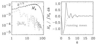
Figure 3: Power spectrum, $M_{k}$, of the magnetic field for an ABC flow dynamo with $A=B=C\equiv U_{0}=1$ and $k=1$. Note that most of the power is in the small scales with $M_{k}\sim k^{1/3}$. The normalised helicity spectrum is also plotted. Note that for medium and large values of $k$ the spectral magnetic helicity is very small; ${\textstyle{1\over 2}}k|H_{k}|\ll M_{k}$. The simulation was done with $240^{3}$ mesh points and a magnetic diffusivity $\eta=2\times 10^{-4}$.

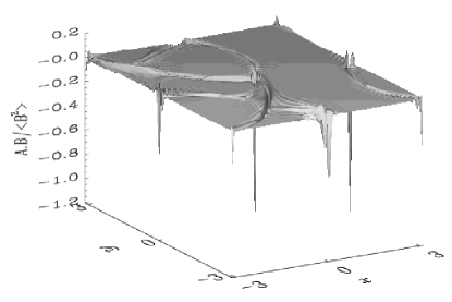
Figure 4: Cross-section of the magnetic helicity density for the ABC flow dynamo from Fig. 3. Note the intermittent nature of ${\bf{A}}\cdot{\bf{B}}$.

Figure 5: Magnetic helicity, $\langle{\bf{A}}\cdot{\bf{B}}\rangle$, nondimensionalised by $\langle{\bf{B}}^{2}\rangle/k_{1}$, as a function of $R_{\rm m}=U_{0}/(\eta k_{1})$ for a model with $A=B=C\equiv U_{0}=1$. Here, $k_{1}=1$ is the smallest wavenumber in the box, which has the size $(2\pi)^{3}$. Note that $k_{1}\langle{\bf{A}}\cdot{\bf{B}}\rangle/\langle{\bf{B}}^{2}\rangle$ decreases with increasing $R_{\rm m}$ like $R_{\rm m}^{-1/2}$. Thus, in the high magnetic Reynolds number limit $1/\eta\to\infty$, the magnetic helicity of the ABC flow dynamo vanishes.

We note in passing that the magnetic power spectrum increases approximately like $k^{1/3}$ (see the left panel of Fig. 3), which is similar to the results from a number of other dynamos as long as they are in the kinematic regime; see, e.g., Fig. 22 of B01 for a large magnetic Prandtl number calculation and Fig. 17 of Brandenburg et al. (1996) for convective dynamos. Thus, most of the spectral magnetic energy is in small scales, which is quite different from the helical turbulence simulations of B01. In turbulent dynamos this spectrum could be explained by the analogy between magnetic field and vorticity (Batchelor 1950). For a Kolmogorov $k^{-5/3}$ spectrum, the vorticity spectrum has a $k^{1/3}$ inertial range. In the present case, however, this argument does not apply because the flow is stationary, so there is no cascade in velocity. Thus, the origin of the $k^{1/3}$ spectrum for these types of kinematic dynamos remains unclear.

One might wonder whether nearly perfect magnetic helicity cancellation can also occur in the sun. Before we can address this question we need to understand the circumstances under which this type of magnetic helicity cancellation can occur. It appears that nearly perfect magnetic helicity cancellation is an artefact of the assumption of linearity and of a small computational domain. Increasing its size allows larger scale fields to grow even though the field has already saturated on the scale of the ABC flow. This is shown in Fig. 6 where we plot the magnetic energy of the mean magnetic field, $\overline{\bf{B}}$, for a ‘nonlinearised’ ABC flow with $A=0$, and $B=C=1/(1+M/M_{0})$, where $M$ is the magnetic energy and $M_{0}=1$. We chose a domain of size $2\pi\times 2\pi\times 8\pi$, which is increased in the $z$ direction by a factor 4. In the kinematic phase the high wavenumber modes grow fastest. Once the magnetic energy reaches saturation, the velocity is decreased, so the high wavenumber modes stop growing, but the remaining lower wavenumber modes are still excited. Although they grew slower during the earlier kinematic stage, they are now still excited and saturate at a much later time. This process continues until the mode with the geometrically largest possible scale has reached saturation, provided that mode remains still excited. Once a large scale field of this form has developed, cancellation of any form has become small. This is indicated by the fact, that the magnetic helicity is nearly maximum, i.e. $H/(2\mu_{0}M)\approx k_{m}^{-1}$ with $k_{m}$ being the momentary wavenumber of the large scale magnetic field, which is also indicated in Fig. 6. Thus, for this type of dynamo, small scale magnetic fields are highly intermittent and can grow fast, while large-scale fields grow once again on slow time scales only. It is this type of large scale field generation that is often thought to be responsible for generating the large scale field of the sun (see Parker 1979, Krause & Rädler 1980, or Zeldovich et al. 1983, for conventional models of the solar dynamo), although the saturation process is still resistively slow.

Figure 6: Evolution of the magnetic energy $M=\langle{\bf{B}}^{2}/2\mu_{0}\rangle$, for a ‘nonlinearised’ ABC flow with $A=0$, and $B=C=1/(1+M/M_{0})$ scales with the magnetic energy, $M$. The box has a side length of $8\pi$ in the $z$ direction. In the kinematic stage ($t<500$) modes with $k>1$ grow fastest. After the small scale modes saturate, the energy of the larger scales continues to grow until the large scale reaches saturation (e.g., $k=0.5$ saturates after $t=2000$). The field continues to grow even further, but very slowly. Since the box has a side length of $8\pi$, the minimum wavenumber is $k=0.25$.

3.2 Magnetic helicity cancellation in turbulent dynamos

Magnetic helicity cancellation seems to be a generic phenomenon of all kinematic dynamos, including the turbulent dynamos in cartesian domains that have been studied recently in B01. Even though the initial field is fully helical, the signs of magnetic helicity are different at large and small scales and can therefore cancel, at least in principle. In practice there remains always some finite net magnetic helicity, but as the magnetic Reynolds number increases, the total magnetic helicity decreases, exactly like for the ABC-flow dynamos studied in Sect. 3.1. Examples of magnetic power spectra calculated separately for the right and left handed parts of the field are shown in Fig. 7 for Runs A, B, and C of Brandenburg & Sarson (2002, hereafter referred to as BS02). These are models with helical forcing around a wavenumber $k_{\rm f}$, like in B01. The basic parameters of the runs presented in BS02 are summarised in Table LABEL:Tsum. Run A has ordinary magnetic diffusivity with $\eta=10^{-4}$, whilst Runs B and C have second order hyperdiffusivity, so $\eta\nabla^{2}{\bf{A}}$ is replaced by $-\eta_{2}\nabla^{4}{\bf{A}}$ in the induction equation (4), and $\eta_{2}=3\times 10^{-8}$ and $10^{-8}$ for Runs B and C, respectively. [Generally, for models with $n$th order hyperdiffusivity, one would have a diffusion term $(-1)^{n+1}\eta_{n}\nabla^{2n}{\bf{A}}$.] In all three cases the forcing of the flow is at wavenumber $k_{\rm f}=27$ with the same amplitude ($f_{0}=0.1$), as in B01. At the forcing scale, Run B is by a factor $\eta_{1}k_{\rm f}^{2}/(\eta_{2}k_{\rm f}^{4})=0.22$ times less resistive than Run A. Run C is another three times less resistive. During the kinematic phase shown, the spectral power increases at all wavenumbers at a rate proportional to $e^{\gamma t}$, where $\gamma=2\lambda$ is the kinematic growth rate of the magnetic energy and $\lambda$ the growth rate of the rms magnetic field.

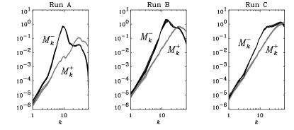
Figure 7: Power spectra separately for the right and left handed parts of the field, for Runs A, B, and C of BS02. Different times have been collapsed onto the same graph by scaling the spectra with $e^{-\gamma t}$, where $\gamma$ is the corresponding growth rate of the magnetic energy for each run. Note that as the magnetic diffusivity is reduced, the relative excess of $M_{k}^{-}$ over $M_{k}^{+}$ decreases, as expected for asymptotic magnetic helicity conservation.

As the magnetic Reynolds number increases, the magnetic helicity normalised by the magnetic energy, $-H/M$, decreases, as shown in Fig. 8 for Runs A, B, and C of BS02. The helicity of the forcing and the kinetic helicity of the flow are positive, so the magnetic helicity at small scales is also positive. This results in large scale magnetic helicity that is negative. Therefore, also the total magnetic helicity is negative.

The asymptotic decrease of magnetic helicity for progressively smaller magnetic diffusivity (Fig. 5) can be quantitatively described by Berger’s (1984) magnetic helicity constraint, which we modify here for the initial kinematic evolution when the magnetic energy increases exponentially at the rate $\gamma=2\lambda$. We consider first the case of ordinary magnetic diffusivity and turn then to the case of hyperdiffusivity. For a closed or periodic domain, the modulus of the time derivative of the magnetic helicity can be bounded from above by

$$\begin{array}[]{lll}\displaystyle{\frac{1}{\mu_{0}}\left|{{\rm d}{}H\over{\rm d}{}t}\right|}=2\eta|\langle{\bf{J}}\cdot{\bf{B}}\rangle|V&\leq&2\eta\langle{\bf{J}}^{2}\rangle^{1/2}\langle{\bf{B}}^{2}\rangle^{1/2}V\\ &=&2\eta^{1/2}Q_{\rm Joule}^{1/2}(2M)^{1/2},\end{array}$$ (46)

where $Q_{\rm Joule}=\langle\eta\mu_{0}{\bf{J}}^{2}\rangle$ is the rate of Joule dissipation. In the kinematic regime, $|\dot{H}|=\gamma|H|$ and $\dot{M}=\gamma M=W-Q_{\rm Joule}=\epsilon Q_{\rm Joule}$, where $W$ is the work done on the magnetic field by the velocity field. In the dynamo case, i.e. if $\gamma>0$, we have $\epsilon>0$. Thus

$${\gamma\over\mu_{0}}|H|\leq 2\eta^{1/2}(\gamma M/\epsilon)^{1/2}(2M)^{1/2}=(2\eta\gamma/\epsilon)^{1/2}(2M)$$ (47)

or

$$|H|/(2\mu_{0}M)\leq\epsilon^{-1/2}(2\eta/\gamma)^{1/2}=a\ell_{\rm skin},$$ (48)

where $\ell_{\rm skin}=(2\eta/\gamma)^{1/2}$ is the skin depth associated with the growth rate $\gamma$ and $a=\epsilon^{-1/2}$ is a parameter describing the fractional excess of magnetic energy gain over dissipation.

In the case of hyperdiffusivity, which is often used for numerical reasons, we have

$$Q_{\rm Joule}\equiv\eta_{n}\int|\mbox{\boldmath$k$}{}|^{2n}{|B_{\mbox{\boldmath$k$}{}}|^{2}\over\mu_{0}}\,d^{3}k\approx\eta_{n}k_{\rm f,eff}^{2n}\left\langle{{\bf{B}}^{2}\over\mu_{0}}\right\rangle V,$$ (49)

where $k_{\rm f,eff}\approx k_{\rm f}$ is an effective wavenumber defined such that the second equality in Eq. (52) below is satisfied exactly and in Eq. (49) only approximately. The rate of change of magnetic helicity is then bounded by

$$\begin{array}[]{lll}\displaystyle{{\gamma\over\mu_{0}}}|H|&\leq&2\eta_{n}\int|\mbox{\boldmath$k$}{}|^{2n-1}|B_{\mbox{\boldmath$k$}{}}|^{2}/\mu_{0}\,d^{3}k\\ &\equiv&2\eta_{n}^{1/2}k_{\rm f,eff}^{n-1}\langle\eta_{n}k_{\rm f,eff}^{2n}{\bf{B}}^{2}/\mu_{0}\rangle^{1/2}\langle{\bf{B}}^{2}/\mu_{0}\rangle^{1/2}V,\end{array}$$ (52)

or

$$\begin{array}[]{lll}\displaystyle{{\gamma\over\mu_{0}}}|H|&\leq&2(\eta_{n}k_{\rm f,eff}^{2n-2})^{1/2}Q_{\rm Joule}^{1/2}(2M)^{1/2}\\ &=&(2\eta_{n}k_{\rm f,eff}^{2n-2})^{1/2}(\gamma/\epsilon)^{1/2}(2M).\end{array}$$ (55)

So, again,

$$|H|/(2M)\leq a\ell_{\rm skin},$$ (56)

but now $\ell_{\rm skin}=(2\eta_{n}k_{\rm f,eff}^{2n-2}/\gamma)^{1/2}$ involves the value of $k_{\rm f,eff}$. Like in the case with ordinary magnetic diffusivity we have $a=\epsilon^{-1/2}$. From the values of $|H|/(2\mu_{0}M)$ and $\ell_{\rm skin}$ given in Table LABEL:Tsum we see that this constraint is indeed well satisfied during the kinematic growth phase.

Table 1: Summary of runs, some of which were already presented in BS02. The runs with $n=2$ have hyperdiffusivity, so the effective diffusivity at the forcing wavenumber, $k_{\rm f}$, and at the Nyquist wavenumber, $k_{\rm Ny}=\pi/\delta x=N/2$, are different. $N^{3}$ is the total number of mesh points, and $\delta x$ is the mesh spacing. The parameter $\ell_{\rm skin}$ gives an approximate upper bound for $|H|/(2\mu_{0}M)$.

Run	$N$	$n$	$\eta_{n}$	$\eta_{n}k_{\rm f}^{2n-2}$	$\eta_{n}k_{\rm Ny}^{2n-2}$	$\gamma$	$k_{\rm f}$	$\alpha_{\rm trav}$	$|H|/(2\mu_{0}M)$	$\ell_{\rm skin}$	$S/(2M)|_{\rm t=1000}$
A	$120^{3}$	1	$10^{-4}$	$10^{-4}$	$10^{-4}$	0.047	27	$1.1\times 10^{-3}$	0.035	0.065	0.00075
B	$120^{3}$	2	$3\times 10^{-8}$	$2\times 10^{-5}$	$10^{-4}$	0.070	27	$7.3\times 10^{-4}$	0.018	0.025	0.00035
C	$120^{3}$	2	$10^{-8}$	$7\times 10^{-6}$	$4\times 10^{-5}$	0.082	27	$3.6\times 10^{-4}$	0.005	0.013	0.00020
D	$30^{3}$	2	$10^{-4}$	$9\times 10^{-4}$	$2\times 10^{-2}$	0.078	3	–	0.08	0.15	–
E	$60^{3}$	2	$10^{-5}$	$2\times 10^{-4}$	$9\times 10^{-3}$	0.12	5	–	0.040	0.065	–
F	$120^{3}$	2	$3\times 10^{-8}$	$3\times 10^{-7}$	$10^{-4}$	0.12	3	–	0.0013	0.0021	–

Figure 8: Magnetic helicity, normalised by the magnetic energy, for Runs A, B, and C of BS02. In Run A, $\eta=10^{-4}$, whereas in Runs B and C second order hyperresistivity is used, with $\eta_{2}=3\times 10^{-8}$ and $10^{-8}$, respectively. Note that the smaller the magnetic diffusivity (at large and intermediate scales), the slower is the saturation of magnetic helicity.

3.3 Magnetic helicity conversion to large scales

At least initially, i.e. when the field is still growing exponentially, there is a strong conversion of positive magnetic helicity at the driving scale to negative magnetic helicity at a certain larger scale. This can be described by the magnetic helicity equation, written separately for positive and negative parts,

$$\dot{H}_{\pm}=\pm 2S-2\eta k_{\pm}^{2}H_{\pm},$$ (57)

where $H_{\pm}=\int H_{k}^{\pm}{\rm d}{}k$, with $k_{\pm}^{n}=\int k^{n}H_{k}^{\pm}{\rm d}{}k/\int H_{k}^{\pm}{\rm d}{}k$, and $S$ describes the transfer of magnetic helicity from small to large scales. In runs with second order hyperresistivity, the term $\eta k_{\pm}^{2}$ has to be replaced by $\eta_{2}k_{\pm}^{4}$. The evolution of the net magnetic helicity, $H^{+}+H^{-}$, is of course unaffected by $S$. We note, however, that the spectrum of the magnetic helicity does have non-diffusive source and sink terms such that its integral over all wavenumbers vanishes (see B01 for detailed plots). The term $\pm S$ in Eq. (57) is related to the $\alpha$ effect (Blackman & Field 2000) or, more precisely, to the turbulent electromotive force. In the present case, where turbulent diffusion also enters, we have therefore (cf. B01)

$$S=\langle\alpha\overline{\bf{B}}^{2}-\eta_{\rm t}\mu_{0}\overline{\bf{J}}\cdot\overline{\bf{B}}\rangle V.$$ (58)

Since the other two terms in Eq. (57) are known, we can directly work out $S$ from this equation. The results for Runs A, B, and C are plotted in Fig. 9. The quantity $S/(2M)$ is a measure of the rate of helicity transfer, i.e. the difference between $\alpha$-effect and turbulent diffusion. Although the ratio $S/(2M)$ has not yet settled to a stationary value, we compare in Table LABEL:Tsum the values for three different runs (at $t=1000$).

Figure 9: Relative magnetic helicity transfer from small to large scales for runs A (most resistive), B and C (least resistive) of BS02, as a function of time. Note that for smaller magnetic diffusivity, the ratio $S/(2M)$ decreases and hence the conversion to large scales becomes less efficient.

Figure 9 shows that $S/(2M)$ approaches a finite value in the nonlinear regime, but its value becomes smaller as the magnetic diffusivity is decreased. Thus, even though strong final field strengths are possible, this can still be achieved with a residual $\alpha$ effect that decreases with decreasing magnetic diffusivity. This is consistent with earlier results of Cattaneo & Vainshtein (1991), Vainshtein & Cattaneo (1992), and Cattaneo & Hughes (1996) that $\alpha$ and $\eta_{\rm t}$ are quenched in a $R_{\rm m}$-dependent fashion. Field & Blackman (2002) have pointed out, however, that this result can also be explained by a dynamically quenched $\alpha$ where $\alpha$ and $\eta_{\rm t}$ are not necessarily quenched in a $R_{\rm m}$-dependent fashion.

Figure 10: Evolution of magnetic energy spectra in the hyperdiffusive Run B in equidistant time intervals from $t=0$ (lowest curve), $t=40$ (next one higher up), until $t=2080$ (peaking at the very top left). The dotted lines give the kinetic energy.

One may wonder whether the $R_{\rm m}$-dependent slow-down during the saturation phase of the large scale field (as seen in Fig. 9), applies also to intermediate scales. In Fig. 10 we show how the magnetic power spectrum shows a bump at intermediate wavenumbers (i.e. the wide maximum at wavenumbers $k<20k_{1}$) travelling to the left toward smaller wavenumbers. In order to check whether or not the speed of the spectral bumps in the different runs shown in Figs 7 and 10 also decreases with decreasing magnetic diffusivity we plot in Fig. 11 the position of the secondary bump in the power spectrum as a function of time. It is evident that the slope, which signifies the speed of the bump, decreases with decreasing magnetic diffusivity. A reasonable fit to this migration is given by

$$k_{\max}^{-1}=\alpha_{\rm trav}(t-t_{\rm sat}),$$ (59)

where the parameter $\alpha_{\rm trav}$ characterises the speed at which this secondary bump travels. The values obtained from fits to various runs are also listed in Table LABEL:Tsum. Following arguments given by Pouquet et al. (1976), $\alpha_{\rm trav}$ obtained in this way is actually a measure of the $\alpha$ effect. The decrease of $\alpha_{\rm trav}$ with decreasing magnetic diffusivity adds to the evidence that the $\alpha$ effect is quenched in a $R_{\rm m}$ dependent fashion.

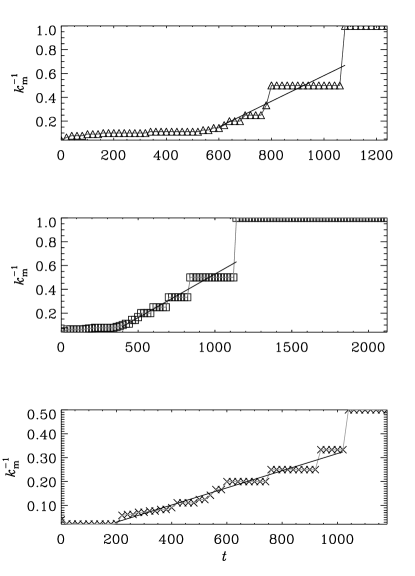
Figure 11: Evolution of the position of the secondary bump in the power spectrum.

The $R_{\rm m}$ dependence of $\alpha_{\rm trav}$ and $S/(2M)$, both indicative of inverse energy transfer, seems to be in conflict with the usual idea of an inverse cascade where such transfers happen on a dynamical time scale (e.g., Verma 2001). The only reasonable conclusion from this seems to be that the (nonlocal!) inverse transfer discussed here is in fact distinct from the usual inverse cascade. In other words, the present simulations do not support the concept of an inverse cascade in the usual (local) sense.

3.4 Magnetically driven turbulence

In the cases considered so far, the turbulence is driven by a forcing term in the momentum equation. Another way to inject energy into the system is by adding an irregular external electromotive force ${\cal E}$${}_{\rm ext}(\mbox{\boldmath$x$}{},t)$ to the system. The induction equation (4) is then replaced by

$$\frac{\partial{\bf{A}}}{\partial t}={\bf{u}}\times{\bf{B}}+\eta\nabla^{2}{\bf{A}}+\mbox{\boldmath${\cal E}$}_{\rm ext}(\mbox{\boldmath$x$}{},t).$$ (60)

This is in some ways reminiscent of turbulence driven by magnetic instabilities (e.g.  the magnetorotational instability, buoyancy or kink instabilities). The direct injection of energy into the induction equation was also considered by Pouquet et al. (1976), for example, who assumed the forcing to be helical. The results of such a run are shown in Fig. 12. Note that the magnetic energy evolves to larger values as the magnetic diffusivity is decreased. This is because the injection of magnetic energy is primarily balanced by magnetic diffusion, which becomes weaker as the magnetic diffusivity is decreased. In the runs with second order hyperdiffusivity (denoted by $\eta_{2}$) the magnetic energy evolves to even larger values. What is more important, however, is the time scale on which saturation is achieved. This time scale is the resistive one, suggesting again that the transport of magnetic energy across the spectrum from small to large scales is a resistively limited process.

Figure 12: Evolution of magnetic energy in runs with magnetic driving. Forcing occurs in the induction equation around wavenumber $k_{\rm f}=5$. Runs with hyperdiffusivity are denoted by $\eta_{2}$ and those with ordinary diffusivity by $\eta_{1}$.

4 Evolution of the large scale magnetic helicity

4.1 Magnetic helicity flux from global mean-field models

The only information available to date about the magnetic helicity of the sun is from surface magnetic fields, and these data are incomplete. Vector magnetograms of active regions show negative (positive) current helicity on the northern (southern) hemisphere (Seehafer 1990, Pevtsov, Canfield, & Metcalf 1995, Bao et al. 1999, Pevtsov & Latushko 2000). From local measurements one can only obtain the current helicity, so nothing can be concluded about magnetic helicity. Typically, however, current and magnetic helicities agree in sign, but the current helicity is stronger at small scales.

Berger & Ruzmaikin (2000) have estimated the flux of magnetic helicity from the solar surface. They discussed $\alpha$-effect and differential rotation as the main agents facilitating the loss of magnetic helicity. Their results indicate that the flux of magnetic helicity due to rotation and the actual magnetic field obtained from solar magnetograms is negative (positive) in the northern (southern) hemisphere. Thus, the sign agrees with that of the current helicity obtained using vector magnetograms. Finally, Chae (2000) estimated the magnetic helicity flux based on counting the crossings of pairs of flux tubes. Combined with the assumption that two nearly aligned flux tubes are nearly parallel, rather than antiparallel, his results again suggest that the magnetic helicity is negative (positive) in the northern (southern) hemisphere.

What is curious here is that even though different scales are involved (small and intermediate scales in active regions and coronal mass ejections, and large scales in the differential rotation), there is as yet no evidence that the helicity spectrum of the sun reverses sign at some scale.

We now discuss the magnetic helicity properties of mean-field $\alpha\Omega$ dynamos in a sphere. There are different reasons why looking at mean-field dynamos can be interesting in connection with helical turbulence. Firstly, magnetic helicity involves one wavenumber factor less than the magnetic energy and tends therefore to be dominated by the large scale field. Magnetic helicity should therefore be describable by mean-field theory. Secondly, mean-field dynamos easily allow the spherical geometry to be taken into account. This is mainly because such models can be only two-dimensional. The resulting field geometry does in some ways resemble the solar field. We recall, however, that at present there is no satisfactory model that explains both the equatorward migration of magnetic activity as well as the approximate antiphase between radial and azimuthal field (${\overline{B}}_{r}{\overline{B}}_{\phi}<0$ during most of the cycle; see Stix 1976), and is still compatible with the observed differential rotation ($\partial\Omega/\partial r>0$ at low latitudes). The sign of differential rotation does not however affect the sign of the magnetic helicity. In fact, the velocity does never generate magnetic helicity, it contributes only to the flux of magnetic helicity; see Eqs (5) and (6).

Table 2: Properties of mean-field dynamos for different signs of $\alpha$ and radial shear, $\Omega^{\prime}=\partial\Omega/\partial r$. All of these models are problematic when applied to the sun. Case (iii), where $\alpha_{0}>0$ and $\Omega^{\prime}<0$, satisfies two important constraints (butterfly diagram with equatorward migration, antiphase between radial and azimuthal field), but it is incompatible with the helioseismology data which indicate that at least at low latitudes $\Omega^{\prime}>0$.

$\Omega^{\prime}<0$ $\Omega^{\prime}>0$ $\alpha_{0}<0$ Case (i) Case (ii) helioseismology not OK helioseismology OK butterfly not OK butterfly OK phase rel. OK phase rel. not OK $H_{\rm N}$ and $Q_{\rm N}$ negative $H_{\rm N}$ and $Q_{\rm N}$ negative $\alpha_{0}>0$ Case (iii) Case (iv) helioseismology not OK helioseismology OK butterfly OK butterfly not OK phase rel. OK phase rel. not OK $H_{\rm N}$ and $Q_{\rm N}$ positive $H_{\rm N}$ and $Q_{\rm N}$ positive

For the axisymmetric mean field, $\overline{\bf{B}}$, of an $\alpha\Omega$ dynamo we calculate the gauge-invariant relative magnetic helicity of Berger & Field (1984) for the northern hemisphere (indicated by N),

$$H_{\rm N}=\int_{\rm N}(\overline{\bf{A}}+\overline{\bf{A}}_{\rm P})\cdot(\overline{\bf{B}}-\overline{\bf{B}}_{\rm P})\;{\rm d}{}V,$$ (61)

where $\overline{\bf{B}}_{\rm P}=\mbox{\boldmath$\nabla$}{}\times\overline{\bf{A}}_{\rm P}$ is a potential reference field inside the northern hemisphere, whose radial component agrees with $\overline{\bf{B}}$ (see Bellan 1999 for a review). This implies that ${\overline{A}}_{\phi}={\overline{A}}_{{\rm P}\phi}$ on the boundary of the northern hemisphere (both on the outer surface and the equator).

In spherical coordinates an axisymmetric magnetic field can be expressed in the form $\overline{\bf{B}}={\overline{B}}_{\phi}\vec{\hat{\phi}}+\mbox{\boldmath$\nabla$}{}\times{\overline{A}}_{\phi}\vec{\hat{\phi}}$. The potential reference field is purely poloidal. Therefore, the dot product of the toroidal components in the integral (61) is simply

$$H_{\rm N}^{\rm(tor)}=\int_{\rm N}({\overline{A}}_{\phi}+{\overline{A}}_{{\rm P}\phi}){\overline{B}}_{\phi}\;{\rm d}{}V.$$ (62)

For the dot products of the poloidal components of the integral we express the magnetic vector potential in the form $\overline{\bf{A}}={\overline{A}}_{\phi}\vec{\hat{\phi}}+\mbox{\boldmath$\nabla$}{}\times{\overline{C}}_{\phi}\vec{\hat{\phi}}$, where $\vec{\hat{\phi}}\cdot\mbox{\boldmath$\nabla$}{}\times\mbox{\boldmath$\nabla$}{}\times({\overline{C}}_{\phi}\vec{\hat{\phi}})={\overline{B}}_{\phi}$. We can then write the integrand for the poloidal component as

$$(\mbox{\boldmath$\nabla$}{}\times{\overline{C}}_{\phi}\vec{\hat{\phi}})\cdot\mbox{\boldmath$\nabla$}{}\times({\overline{A}}_{\phi}-{\overline{A}}_{{\rm P}\phi})\vec{\hat{\phi}}={\overline{B}}_{\phi}({\overline{A}}_{\phi}-{\overline{A}}_{{\rm P}\phi})$$

$$-\mbox{\boldmath$\nabla$}{}\cdot[\overline{\bf{A}}\times({\overline{A}}_{\phi}-{\overline{A}}_{{\rm P}\phi})\vec{\hat{\phi}}].$$ (63)

(Note that ${\overline{C}}_{{\rm P}\phi}=0$, as the potential reference field is purely poloidal.) The integral over the divergence term vanishes because ${\overline{A}}_{\phi}={\overline{A}}_{{\rm P}\phi}$ on the boundary, so we have

$$H_{\rm N}^{\rm(pol)}=\int_{\rm N}{\overline{B}}_{\phi}({\overline{A}}_{\phi}-{\overline{A}}_{{\rm P}\phi})\;{\rm d}{}V,$$ (64)

and hence

$$H_{\rm N}=2\int_{\rm N}{\overline{A}}_{\phi}{\overline{B}}_{\phi}\;{\rm d}{}V.$$ (65)

The time evolution of $H_{\rm N}$ can be obtained from the mean-field dynamo equation (e.g. Krause & Rädler 1980), which gives

$${\rm d}{}H_{\rm N}/{\rm d}{}t=2S-Q_{\rm N},$$ (66)

where $S=\int_{\rm N}\overline{\mbox{\boldmath${\cal E}$}}{}\cdot\overline{\bf{B}}\;{\rm d}{}V$ was already defined in Eq. (58), $\overline{\mbox{\boldmath${\cal E}$}}{}=\alpha\overline{\bf{B}}-\eta_{\rm T}\mu_{0}\overline{\bf{J}}$ is the e.m.f. of the mean field, and $Q_{\rm N}$ is the integrated magnetic helicity flux out of the northern hemisphere (i.e. through the outer surface and the equator), with

$$Q_{\rm N}=-2\oint[(\overline{\mbox{\boldmath${\cal E}$}}{}+\overline{\bf{U}}\times\overline{\bf{B}})\times{\overline{A}}_{\phi}\vec{\hat{\phi}}]\cdot{\rm d}{}{\bf{S}},$$ (67)

where $\overline{\bf{U}}=r\sin\theta\,\Omega\vec{\hat{\phi}}$ is the mean toroidal flow. It will be of interest to split $Q_{\rm N}$ into the contributions from the outer surface integral, $Q_{\rm NS}$, and the equatorial plane, $Q_{\rm Eq}$, so $Q_{\rm N}=Q_{\rm NS}+Q_{\rm Eq}$.

In Table LABEL:Taosum we summarise the key properties of typical $\alpha\Omega$ dynamo models for different signs of $\alpha$ and $\Omega^{\prime}\equiv\partial\Omega/\partial r$ (cf. Stix 1976). Here we have also indicated the sign of the magnetic helicity flux that leaves from the northern hemisphere, $Q_{\rm N}$. In all the models presented here the sign of $Q_{\rm N}$ agrees with that of $H_{\rm N}$, which also agrees with the sign of $\alpha$. This is because, averaged over one cycle, $\langle{\rm d}{}H_{\rm N}/{\rm d}{}t\rangle_{\rm cyc}$ vanishes, so the sign of $\langle Q_{\rm N}\rangle_{\rm cyc}$ must agree with that of $\langle S\rangle_{\rm cyc}$ which, in turn, is determined by the sign of $\alpha$; see Eq. (66).

What remains unclear, however, is whether the negative current helicity observed in the northern hemisphere is indicative of small or large scales, and hence whether the sign of $\alpha$ is positive (case iv) or negative (case ii), respectively. Only in case (iv) there would be the possibility of shedding magnetic helicity of the opposite sign; see Sect. 4.3 below. In case (iii), $H_{\rm N}$ is also positive, but here $\Omega^{\prime}<0$, which does not apply to the sun. In case (ii), on the other hand, $H_{\rm N}$ is negative, so shedding of negative magnetic helicity would act as a loss.

Our goal is to estimate the amount of magnetic helicity that is to be expected for more realistic models of the solar dynamo. We also need to know which fraction of the magnetic field takes part in the 11-year cycle. In the following we drop the subscript N on $H$ and $M$. For an oscillatory dynamo, all three variables, $H$, $M$, and $Q_{\rm Joule}$ vary in an oscillatory fashion with a cycle frequency $\omega$ of magnetic energy (corresponding to 11 years for the sun – not 22 years), so we estimate $|{\rm d}{}H/{\rm d}{}t|\mathrel{\mathchoice{\vbox{\offinterlineskip\halign{\hfil$\displaystyle#$\hfil\cr<\cr\sim\cr}}}{\vbox{\offinterlineskip\halign{\hfil$\textstyle#$\hfil\cr<\cr\sim\cr}}}{\vbox{\offinterlineskip\halign{\hfil$\scriptstyle#$\hfil\cr<\cr\sim\cr}}}{\vbox{\offinterlineskip\halign{\hfil$\scriptscriptstyle#$\hfil\cr<\cr\sim\cr}}}}\omega|H|$ and $Q_{\rm Joule}\mathrel{\mathchoice{\vbox{\offinterlineskip\halign{\hfil$\displaystyle#$\hfil\cr<\cr\sim\cr}}}{\vbox{\offinterlineskip\halign{\hfil$\textstyle#$\hfil\cr<\cr\sim\cr}}}{\vbox{\offinterlineskip\halign{\hfil$\scriptstyle#$\hfil\cr<\cr\sim\cr}}}{\vbox{\offinterlineskip\halign{\hfil$\scriptscriptstyle#$\hfil\cr<\cr\sim\cr}}}}\omega M$, which, by arguments analogous to those used in Sect. 3.2, leads to the inequality

$$|H|/(2\mu_{0}M)\leq\ell_{\rm skin},$$ (68)

where $\ell_{\rm skin}=(2\eta/\omega)^{1/2}$ is the skin depth, now associated with the oscillation frequency $\omega$. Thus, the maximum magnetic helicity that can be generated and dissipated during one cycle is characterised by the length scale $|H|/(2\mu_{0}M)$, which has to be less than the skin depth $\ell_{\rm skin}$.

Table 3: Results from a mean-field dynamo model in a spherical shell with outer radius $R$ and inner radius $0.7R$, with either purely latitudinal shear ‘(lat)’ or purely radial shear ‘(rad)’. The values of $\alpha$ given here (in units of $\eta_{\rm T}/R$) lead to dynamos that are only slightly supercritical. The cycle period, $T_{\rm cyc}$, is given in non-dimensional form and would correspond to $22\,{\rm yr}$ for $\eta_{\rm T}=2.4\times 10^{11}\,{\rm cm}^{2}/\,{\rm s}$ (for the models with latitudinal shear), or $3.7\times 10^{11}\,{\rm cm}^{2}/\,{\rm s}$ (for the models with radial shear). The range of ${\overline{B}}_{\rm pole}/{\overline{B}}_{\rm belt}$ that is consistent with observations, $(2\ldots 5)\times 10^{-4}$, is highlighted in bold face. Both $M_{\rm N}$ and $H_{\rm N}$ vary with the dynamo cycle period; $H_{\rm N}^{\max}$ and $\langle H_{\rm N}\rangle$ refer to the maximum and time averaged values of $H_{\rm N}$, respectively. $\langle Q_{\rm NS}\rangle T_{\rm cyc}$ is the outwards magnetic helicity flux through the northern surface, while $\langle Q_{\rm Eq}\rangle T_{\rm cyc}$ is the magnetic helicity flux through the equator into the southern hemisphere.

$C_{\alpha}$ $C_{\Omega}$ $\displaystyle{{\overline{B}}_{\rm pole}\over{\overline{B}}_{\rm belt}}$ $\displaystyle{H_{\rm N}^{\max}\over 2\mu_{0}M_{\rm N}R}$ $\displaystyle{\langle H_{\rm N}\rangle\over 2\mu_{0}M_{\rm N}R}$ $\displaystyle{\langle Q_{\rm NS}\rangle T_{\rm cyc}\over{\overline{B}}_{\rm belt}^{2}R^{4}}$ $\displaystyle{\langle Q_{\rm Eq}\rangle T_{\rm cyc}\over{\overline{B}}_{\rm belt}^{2}R^{4}}$ $\displaystyle{T_{\rm cyc}\eta_{\rm T}\over R^{2}}$ $2\times 10^{-1}$ $1\times 10^{5}$ (lat) $\bf 1\times 10^{-3}$ $1\times 10^{-3}$ $4\times 10^{-4}$ $6\times 10^{-4}$ $7\times 10^{-6}$ 0.030 $6\times 10^{-2}$ $3\times 10^{5}$ (lat) $\bf 3\times 10^{-4}$ $3\times 10^{-4}$ $1\times 10^{-4}$ $2\times 10^{-4}$ $2\times 10^{-6}$ 0.030 $2\times 10^{-2}$ $1\times 10^{6}$ (lat) $1\times 10^{-4}$ $1\times 10^{-4}$ $4\times 10^{-4}$ $6\times 10^{-5}$ $7\times 10^{-7}$ 0.030 $2\times 10^{-0}$ $3\times 10^{3}$ (rad) $\bf 8\times 10^{-4}$ $5\times 10^{-3}$ $5\times 10^{-3}$ $6\times 10^{-4}$ $2\times 10^{-3}$ 0.047 $6\times 10^{-0}$ $1\times 10^{4}$ (rad) $\bf 2\times 10^{-4}$ $2\times 10^{-3}$ $1\times 10^{-3}$ $3\times 10^{-4}$ $5\times 10^{-4}$ 0.047 $2\times 10^{-1}$ $3\times 10^{4}$ (rad) $8\times 10^{-5}$ $5\times 10^{-4}$ $5\times 10^{-4}$ $7\times 10^{-5}$ $2\times 10^{-4}$ 0.047

For $\eta$ we have to use the Spitzer resistivity which is proportional to $T^{-3/2}$ ($T$ is temperature), so $\eta$ varies between $10^{4}\,{\rm cm}^{2}/\,{\rm s}$ at the base of the convection zone to about $10^{7}\,{\rm cm}^{2}/\,{\rm s}$ near the surface layers and decreases again in the solar atmosphere. Using $\omega=2\pi/(11\,{\rm yr})=2\times 10^{-8}\,{\rm s}^{-1}$ for the relevant frequency at which $H$ and $M$ vary we have $\ell_{\rm skin}\approx 10\,{\rm km}$ at the bottom of the convection zone and $\ell_{\rm skin}\approx 300\,{\rm km}$ at the top. This needs to be compared with the value $|H|/(2\mu_{0}M)$ obtained from dynamo models.

In order to see how the condition (68) is met by mean-field models, we present the results from a typical $\alpha\Omega$ model of the solar dynamo. Although mean-field theory has been around for several decades, the helicity aspect has only recently attracted attention. In the proceedings of a recent meeting devoted specifically to this topic (Brown, Canfield, & Pevtsov 1999) helicity was discussed extensively also in the context of mean-field theory. However, the possibility of helicity reversals at some length scale was not addressed at the time. We recall that in the Babcock–Leighton approach it is mainly the latitudinal differential rotation that enters. We also note that, although the latitudinal migration could be explained by radial differential rotation, meridional circulation is in principle able to drive meridional migration even when the sense of radial differential rotation would otherwise be wrong for driving meridional migration (Durney 1995, Choudhuri, Schüssler, & Dikpati 1995, Küker, Rüdiger, & Schultz 2001). We therefore proceed with the simplest possible model in spherical geometry. An example of the resulting butterfly diagrams of toroidal field, magnetic helicity and magnetic helicity flux is shown in Fig. 13.

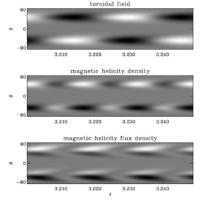
Figure 13: Butterfly diagrams of the toroidal field from a mean field model, compared with butterfly diagrams of the magnetic helicity density near the surface and magnetic helicity flux due to differential rotation at the surface. Note that the local magnetic helicity density is most of the time positive (light grey) in the northern hemisphere and negative (dark grey) in the southern hemisphere. The magnetic helicity flux shows a similar variation, but there is a certain degree of cancellation taking place at any moment in time. $C_{\alpha}=0.175$, $C_{\Omega}=1\times 10^{5}$ (lat).

The main parameters that can be changed in the model are $\alpha_{0}$ (we assume that $\alpha=\alpha_{0}\cos\theta$, where $\theta$ is colatitude), $\eta_{\rm T}$ (=const), and the magnitude of the angular velocity, $\Omega_{0}$, in the expression

$$\Omega=\Omega_{0}\left[1-0.038{P_{3}^{1}(\cos\theta)\over\sin\theta}-0.004{P_{5}^{1}(\cos\theta)\over\sin\theta}\right],$$ (69)

which is a fit that resembles closely the surface angular velocity of the sun (Rüdiger 1989). What matters for the axisymmetric dynamo is only the pole–equator difference, $\Delta\Omega$, which is about a third of $\Omega_{0}$. Our model is made dimensionless by putting $R=\eta_{\rm T}=1$. The governing non-dimensional parameters are $C_{\alpha}=\alpha_{0}R/\eta_{\rm T}$ and $C_{\Omega}=\Delta\Omega R^{2}/\eta_{\rm T}$, where $\Delta\Omega=\Omega_{\max}-\Omega_{\min}$. This leads to the observables ${\overline{B}}_{\rm pole}$, by which we mean the radial field at the pole, which is about 2 gauss for the sun, and ${\overline{B}}_{\rm belt}$, by which we mean the azimuthal field in the main sunspot belts. The solar value of ${\overline{B}}_{\rm belt}$ is estimated to be around $4\ldots 8\,{\rm kG}$, based on equipartition arguments and on the total emergent flux during one cycle. Thus, we expect ${\overline{B}}_{\rm pole}/{\overline{B}}_{\rm belt}$ to be in the range $(2\ldots 5)\times 10^{-4}$.

From the model results shown in Table LABEL:Ttimescale we see that, once ${\overline{B}}_{\rm pole}/{\overline{B}}_{\rm belt}$ is in the range consistent with observations, (highlighted in bold face), $\langle H_{\rm N}\rangle/(2\mu_{0}M_{\rm N}R)$ is around $(1\ldots 3)\times 10^{-4}$ for models with latitudinal shear using Eq. (69). Given that $R=700\,{\rm Mm}$ this means that $H_{\rm N}/(2\mu_{0}M_{\rm N})\approx 70\dots 200\,{\rm km}$, which would be compatible with $\ell_{\rm skin}$ only near the top of the convection zone.

In units of ${\overline{B}}_{\rm belt}^{2}R^{4}$, the magnetic helicity flux through the northern hemisphere is about $(2\ldots 5)\times 10^{-4}$. Using typical parameters for the sun, ${\overline{B}}_{\rm belt}=4\,{\rm kG}$ and $R=700\,{\rm Mm}$, we have ${\overline{B}}_{\rm belt}^{2}R^{4}=4\times 10^{50}\,{\rm Mx}^{2}$. Thus, our models predict magnetic helicity fluxes of about $(1\ldots 2)\times 10^{47}\,{\rm Mx}^{2}$ for a full 22 year magnetic cycle, or half of that for the 11 year activity cycle. This is comparable to the values reported by Berger & Ruzmaikin (2000), but less that those given by DeVore (2000). Significant magnetic helicity fluxes through the equator are only found if angular velocity contours cross the equatorial plane, i.e. in the models with radial differential rotation.

If the observed negative magnetic helicity flux on the northern hemisphere is associated with the large scale field, it would suggest that $\alpha_{0}<0$. This corresponds to case (ii), where magnetic helicity flux would contribute as an additional loss of large scale magnetic energy. On the other hand, if the observed negative magnetic helicity flux is associated with the small scale field, it could remove excess magnetic helicity of the opposite sign, which may act as a source of large scale magnetic energy; see Sect. 4.3. This corresponds to case (iv) where $\alpha_{0}>0$.

4.2 Balance equations

The models with imposed positive helical forcing at small length scale show clearly that there is a production of equal amounts of positive and negative magnetic helicity at small and large scales, respectively (or vice versa if the helicity of the forcing is negative). As time goes on, more and more positive and negative magnetic helicity builds up on small and large scales. Of course, magnetic helicity always implies magnetic energy as well (this is related to the realisability condition; see Sect. 2.2 and Moffatt 1978), and eventually the value of the small scale magnetic energy will have reached the value of the kinetic energy at that scale, so the dynamo reaches saturation. This happens first at small scales, and if that was where the dynamo stops, the resulting field would be governed by small scales (Kulsrud & Anderson 1992). However, this is not what happens in the majority of the numerical experiments, and probably also not in real astrophysical bodies like the sun.

Before we go on, we need to address the question of opposite helicities in the two hemispheres of astrophysical dynamos. For reasons of symmetry, the total magnetic helicity is always close to zero. It is then convenient to think of the two hemispheres as two systems coupled with each other through an open boundary (the equatorial plane). The equation of magnetic helicity conservation has an additional flux term, $Q$, on the right hand side, so it reads [cf. Eq. (5)]

$${{\rm d}{}H\over{\rm d}{}t}=-2\eta C-Q,$$ (70)

where $H$ is the magnetic helicity, $C$ the current helicity, $\eta$ the microscopic magnetic diffusivity, and $Q$ the magnetic helicity flux integrated over the surface of the given subvolume (i.e. a hemisphere in this case). We are interested in the evolution of the large scale field $\overline{\bf{B}}$, and we refer to the magnetic helicity of this large scale or mean field as $H_{\rm m}$.

In the absence of boundaries we have $H_{\rm m}=\int\overline{\bf{A}}\cdot\overline{\bf{B}}\,{\rm d}{}V$, where $\overline{\bf{B}}=\mbox{\boldmath$\nabla$}{}\times\overline{\bf{A}}$ and overbars denote a suitable average that commutes with the curl operator and satisfies the Reynolds rules (in particular, the average of fluctuations vanishes and the average of an average gives the same; see Krause & Rädler 1980). With open boundaries, however, $\int\overline{\bf{A}}\cdot\overline{\bf{B}}\,{\rm d}{}V$ is no longer gauge invariant. For the present discussion we only need the fact that it is possible to define gauge-invariant versions of magnetic helicity; see Berger & Field (1984) for the three-dimensional case and BD01 (or Sect. 2.4) for the one-dimensional case that is relevant to horizontally averaged fields.

Splitting the field into contributions from mean and fluctuating components we can write

$${{\rm d}{}H_{\rm m}\over{\rm d}{}t}+{{\rm d}{}H_{\rm f}\over{\rm d}{}t}=-2\eta C_{\rm m}-2\eta C_{\rm f}-Q_{\rm m}-Q_{\rm f}.$$ (71)

This equation only becomes useful if we can make appropriate simplifications. BD01 considered the case where the small scale field has already reached saturation and the large scale magnetic energy continues to build up further until it too reaches saturation.

If the large scale field is nearly fully helical we have $M_{\rm m}\approx{\textstyle{1\over 2}}k_{\rm m}|H_{\rm m}|$, where $k_{\rm m}$ is the typical wavenumber of the mean field. Furthermore, if the small scale field is nearly fully helical, too, we have $M_{\rm f}={\textstyle{1\over 2}}k_{\rm f}|H_{\rm f}|$, where $k_{\rm f}$ is the typical wavenumber of the fluctuating field, or the forcing wavenumber, as in B01. Analogous relations link $C$ to $H$. The relative ordering of the ratios of large and small scale magnetic energies relative to magnetic and current helicities is given by

$${|H_{\rm m}|\over|H_{\rm f}|}\approx{k_{\rm f}\over k_{\rm m}}{M_{\rm m}\over M_{\rm f}}\approx\left({k_{\rm f}\over k_{\rm m}}\right)^{2}{|C_{\rm m}|\over|C_{\rm f}|}.$$ (72)

Thus, if $k_{\rm m}\ll k_{\rm f}$, as is usually the case when there is some degree of scale separation, and $M_{\rm m}\approx M_{\rm f}$, we have $|H_{\rm m}|\gg|H_{\rm f}|$ and $|C_{\rm m}|\ll|C_{\rm f}|$, so we are left with

$${{\rm d}{}H_{\rm m}\over{\rm d}{}t}\approx-2\eta C_{\rm f}-2Q_{\rm m}-2Q_{\rm f},$$ (73)

or, using the above estimates between $M$, $H$ and $C$, and assuming, for definiteness, that $H_{\rm m},C_{\rm m}>0$ and $H_{\rm f},C_{\rm f}<0$ (as expected in the northern hemisphere of the sun), we have

$${{\rm d}{}M_{\rm m}\over{\rm d}{}t}\approx+2\eta k_{\rm m}k_{\rm f}M_{\rm f}-2k_{\rm m}Q_{\rm m}-2k_{\rm m}Q_{\rm f}.$$ (74)

(The factor 2 in front of the $Q$s comes from the 1/2 in the definition of $M$.) We can apply this equation to the problem with open boundaries.

However before doing this, we recall that in the absence of any surface fluxes of helicity ($Q=0$) the assumption $M_{\rm m}=M_{\rm f}$ does not apply near saturation. Instead, steadiness of $H$ immediately requires $C=C_{\rm m}+C_{\rm f}=0$, so $|C_{\rm m}|=|C_{\rm f}|$, and hence $M_{\rm m}=(k_{\rm f}/k_{\rm m})\,M_{\rm f}\gg M_{\rm f}$, and $|H_{\rm m}|\gg|H_{\rm f}|$ for the final state. Before this final state is reached we have from Eq. (71)

$${{\rm d}{}M_{\rm m}\over{\rm d}{}t}\approx+2\eta k_{\rm m}k_{\rm f}M_{\rm f}-2\eta k_{\rm m}^{2}M_{\rm m},$$ (75)

which has the solution (B01)

$$M_{\rm m}\approx{k_{\rm f}\over k_{\rm m}}M_{\rm f}\,\left[1-e^{-2\eta k_{\rm m}^{2}(t-t_{\rm s})}\right].$$ (76)

This equation is referred to as the magnetic helicity constraint, which is probably obeyed by all helicity-driven large scale dynamos. Note, however, that no mean-field theory has been invoked here. Equation (76) implies that full saturation is reached not earlier than after a resistive time scale, $(\eta k_{\rm m}^{2})^{-1}$. We emphasise that this is the resistive time scale connected to the large length scale $2\pi/k_{\rm m}$. We also emphasise that this result is unaffected by turbulent or other (e.g. ambipolar; see BS00) magnetic diffusion.

Coming back to the problem with open boundaries we can carry out a similar analysis by relating $Q_{\rm m}$ to the mean field. Based on dimensional arguments we may assume

$$|Q_{\rm m}|=M_{\rm m}/(k_{\rm m}\tau_{\rm m}),$$ (77)

where $\tau_{\rm m}$ is some damping time for the large scale field. We can express this in terms of an effective (turbulent-like) magnetic diffusion coefficient, $\eta_{\rm m}$, for the large scale field, e.g. in the form

$$2\eta_{\rm m}=(\tau_{\rm m}k_{\rm m}^{2})^{-1}\quad\mbox{(definition of $\eta_{\rm m}$)},$$ (78)

so Eq. (74) becomes

$${{\rm d}{}M_{\rm m}\over{\rm d}{}t}\approx+2\eta k_{\rm m}k_{\rm f}M_{\rm f}-2\eta_{\rm m}k_{\rm m}^{2}M_{\rm m}-2k_{\rm m}Q_{\rm f},$$ (79)

which has the solution

$$M_{\rm m}\approx{2\eta k_{\rm f}M_{\rm f}-2Q_{\rm f}\over 2\eta_{\rm m}k_{\rm m}}\,\left[1-e^{-2\eta_{\rm m}k_{\rm m}^{2}(t-t_{\rm s})}\right].$$ (80)

We expect $\eta_{\rm m}$ to scale with the turbulent magnetic diffusivity, $\eta_{\rm t}$, which describes the spreading of the mean magnetic field. This equation yields the time scale $(\eta_{\rm m}k_{\rm m}^{2})^{-1}$, which is indeed shorter than the resistive time scale, $(\eta k_{\rm m}^{2})^{-1}$. However, if $Q_{\rm f}=0$ in Eq. (80), the energy of the final field relative to the small scale field is decreased by the factor $(\eta k_{\rm f})/(\eta_{\rm m}k_{\rm m})\ll 1$. This was the basic result of BD01 where $|Q_{\rm f}|$ was found to be much smaller than $|Q_{\rm m}|$. In other words, all the magnetic large scale helicity loss occurred at large scales, which is of course the scale where we wanted to generate the large scale field.

The above results have shown that magnetic helicity losses due to large scale magnetic fields are not really a satisfactory solution to the problem of generating strong large scale magnetic fields on fast enough time scales. Rather, one requires that there should be a loss of magnetic helicity due to small scale magnetic fields, i.e. a non zero $Q_{\rm f}$. We may assume that $Q_{\rm f}$ and $Q_{\rm m}$ have opposite sign, because both current and magnetic helicities also have different signs for the contributions from small and large scales. Looking back at Eq. (80) is it clear that the $Q_{\rm f}$ term in the numerator can in principle enhance and even completely supersede the resistively limited ‘driver’, $2\eta k_{\rm f}M_{\rm f}$, provided $Q_{\rm f}<0$ on the northern hemisphere.

Physically speaking, the role of small scale magnetic helicity flux is to let the large scale field build up independently of any constraints related to the small scales. To prevent then excessive build-up of magnetic energy at small (and intermediate) scales, which diffusion was able to do (albeit slowly), we need to have another more direct mechanism that is independent of microscopic magnetic diffusion. In order to investigate the problem of excess magnetic helicity at small scales we have performed a series of numerical experiments by Fourier filtering the field and removing in regular time intervals the magnetic energy at the forcing and smaller scales.

4.3 Removing excess magnetic helicity

According to our working hypothesis, the reason why the large scale field can only develop slowly is that the build-up of the large scale field with one sign of magnetic helicity requires the simultaneous build-up (and eventual removal) of small scale field with opposite magnetic helicity. Instead of waiting for ohmic field destruction one might expect that also the explicit removal of magnetic energy at small scales would be able to accomplish this goal.

A more formal argument is this. We use again Eq. (71), but without ignoring the ${\rm d}{}H_{\rm f}/{\rm d}{}t$ term, and make the assumption that large and small scale fields are fully helical, and ignore surface terms, because boundary conditions are assumed periodic. Thus, we have an additional ${\rm d}{}M_{\rm f}/{\rm d}{}t$ term in Eq. (75), which then reads

$${{\rm d}{}M_{\rm m}\over{\rm d}{}t}\approx{k_{\rm m}\over k_{\rm f}}{{\rm d}{}M_{\rm f}\over{\rm d}{}t}+2\eta k_{\rm m}k_{\rm f}M_{\rm f}-2\eta k_{\rm m}^{2}M_{\rm m}.$$ (81)

After small scale magnetic energy is removed, the right hand side of Eq. (81) is out of balance. If we ignored the ${\rm d}{}M_{\rm f}/{\rm d}{}t$ term, the large scale magnetic energy would decay proportional to $-2\eta k_{\rm m}^{2}M_{\rm m}$, because the $2\eta k_{\rm m}k_{\rm f}M_{\rm f}$ term is still negligible after having set $M_{\rm f}=0$. However, the $M_{\rm f}$ term begins to recover immediately which gives rise to a significant contribution from the ${\rm d}{}M_{\rm f}/{\rm d}{}t$ term. Both terms enter with the same sign. If the magnetic Reynolds number is large, i.e. if the recovery rate of $M_{\rm f}$ is faster than than the microscopic decay time, we have a net gain. This is indeed borne out by the simulations, where magnetic energy is removed above the wavenumber $k=4$ every $\Delta t=0.12\lambda^{-1}$ time units, labelled (a) in Fig. 14, and $\Delta t=0.4\lambda^{-1}$, labelled (b). Here, $\lambda=0.07u_{\rm rms}k_{\rm f}$ is the kinematic growth rate of the rms field strength. Shorter time intervals do not give any further enhancement; the resulting curve for $\Delta t=0.04\lambda^{-1}$ lies almost on top of the curve (a) that starts at $\lambda t=80$.

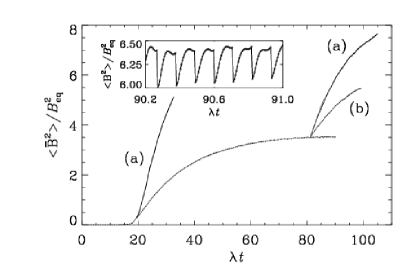
Figure 14: The effect of removing small scale magnetic energy in regular time intervals $\Delta t$ on the evolution of the large scale field (solid lines). The dashed line gives the evolution of $\langle\overline{\bf{B}}^{2}\rangle$ for Run 3 of B01 (where no such energy removal was included) in units of $B_{\rm eq}^{2}=\mu_{0}\rho_{0}\langle{\bf{u}}^{2}\rangle$. The two solid lines show the evolution of $\langle\overline{\bf{B}}^{2}\rangle$ after restarting the simulation from Run 3 of B01 at $\lambda t=20$ and $\lambda t=80$. Time is scaled with the kinematic growth rate $\lambda$. The curves labelled (a) give the result for $\Delta t=0.12\lambda^{-1}$ and those labelled (b) for $\Delta t=0.4\lambda^{-1}$. The inset shows, for a short time interval, the sudden drop and subsequent recovery of the total (small and large scale) magnetic energy in regular time intervals.

We may thus conclude that the preferential removal of small scale magnetic fields does indeed enhance large scale dynamo action. Earlier experiments, which are not reported here, where $k_{\rm f}$ was larger, and therefore the magnetic Reynolds number $u_{\rm rms}/\eta k_{\rm f}$ smaller, did not show such an enhancement. Note however that we still do not really know whether the preferential loss of such small scale field does operate in real astrophysical bodies. Simulations have so far been unsuccessful in demonstrating this. Those presented in BD01 show that most of the magnetic helicity is lost through the large scale field. A possible reason may be that the large scale field geometry was not optimal and that in other settings large scale losses are reduced.

The intermediate scales are probably those where most of the magnetic helicity loss from the sun occurs. This argument is based in particular on the sign of the flux of magnetic helicity on the solar surface: it is found to be negative (positive) on the northern (southern) hemisphere (see §4.1 above).

According to conventional mean-field theory the sign of the $\alpha$-effect should be positive in the northern hemisphere, so the sign of large scale magnetic helicity and the flux thereof should be positive. A reversal of the sign of magnetic helicity can then be expected on some scale smaller than the large scale of the dynamo wave ($100\mbox{--}300\,{\rm Mm}$). Thus, the helicity flux occurs on the scale of active and bipolar regions as well as the scale of coronal mass ejections, which is about $20\mbox{--}50\,{\rm Mm}$. These scales may therefore well correspond to the intermediate scales referred to above. On the other hand, there is some uncertainty as to whether the dynamo alpha in the northern hemisphere of the sun might in fact be negative. If the dynamo $\alpha$ is negative in the northern hemisphere, the magnetic helicity loss on the sun would be of the same sign as that of the large scale dynamo-generated field, so its scale would still belong to the large scales. However, the solution to the helicity problem would then probably not be related to magnetic helicity flux, because then $Q_{\rm f}$ and $Q_{\rm m}$, as well as $H_{\rm m}$, would have the same sign, so $Q_{\rm f}$ would constitute an additional loss term, which does hence not accelerate the dynamo (BD01); see also Sect. 4.

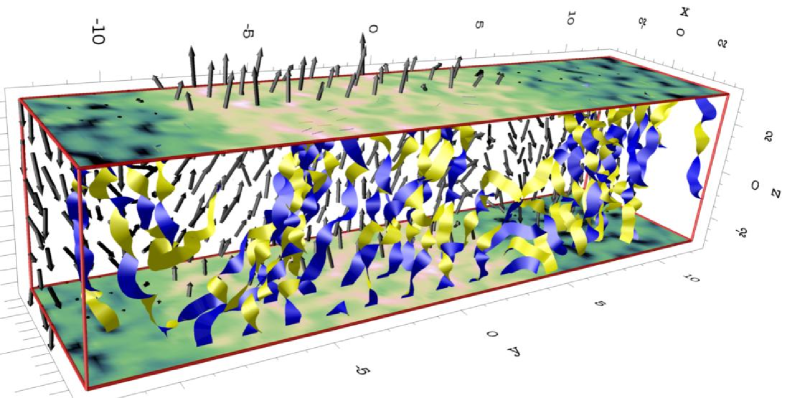
Figure 15: Three-dimensional visualisation of the magnetic field for a simulation where the box is four times longer in the $y$-direction. Vectors in the back half of the box show the orientation of the locally averaged field. Ribbons in the front half indicate magnetic field lines; their twist reflects the local torsality (or helicity) of the magnetic field and has been enhanced artificially by factor of 15. The vertical magnetic field component is indicated by bright (positive) or dark (negative) colours in the top and bottom face of the box.

4.4 Large aspect ratio simulations

In order to assess the role of intermediate scales, we now extend the simulations of BD01 with open boundaries to domains that are larger in one horizontal coordinate direction compared to before. We have already mentioned in the introduction that the simulations of BD01 produced most of the magnetic helicity at large scale, i.e. the same scale as that of the large scale field that we want to build up fast. A potential problem with these simulations could be a lack of sufficient scale separation. In particular, it is conceivable that intermediate scales are not sufficiently well represented in these simulations. The intermediate length scales can be expected to be where most of the magnetic helicity of the opposite sign resides (‘opposite’ is here meant to be relative to the large scale field).

In order to study the possible role of the allowance of intermediate length scales in the simulations we extend the simulations of BD01 to the case of larger aspect ratio. The hope is that the large scale field will now develop in the coordinate direction that is longest, but that most of the magnetic helicity flux occurs still at a similar scale as before and that the sign of magnetic helicity and its flux are now reversed relative to the helicity at the scale of the mean field. In the simulations of BD01 a box with unit aspect ratio was considered, and one of the coordinate directions (the $z$-direction) was non-periodic and magnetic helicity flux through these boundaries occurred. We have now extended this study to the case where the box is four times larger in one of the other directions (the $y$-direction). A three-dimensional visualisation of the resulting field is shown in Fig. 15. The $y$ component of the magnetic field on the $z$-boundaries shows a clear large scale pattern with a length scale larger than the extent of the domain in the $x$ direction. The evolution of the magnetic and kinetic energies of one such run is shown in Fig. 16. We see that kinetic and magnetic energies are approximately in equipartition. The large scale magnetic energy shows, as expected, variation in the $y$ direction, i.e. the wave vector of the large scale field points in the long direction of the box.

Figure 16: Evolution of kinetic and magnetic energies. The magnetic energy contained in the large scale field (averaged in the $x$ and $z$ directions, and denoted by $K_{y}$) is shown as a dash-dotted line. The dotted and dashed curves denote the $z$- and $x$-dependent components, respectively.

Figure 17: Comparison of the evolution of the large scale magnetic field component that varies in the $y$-direction (the direction in which the box is longest) for runs with different aspect ratios, $A$, and different values of $\eta_{-3}=\eta/10^{-3}$. Note the development of a stronger large scale field for $A=1$ than for $A=4$.

Table 4: Summary of the main properties of the runs with vertical field boundary condition. The parameter $q_{j}$ gives the fractional magnetic energy in the mean field relative to the total magnetic field.

$\!\!\!A\!\!\!$ $\!\!\nu\!\!$ $\!\!\eta\!\!$ $\!\!u_{\rm rms}\!\!$ $\!\!b_{\rm rms}\!\!$ $q_{z}\!\!$ $\!\!q_{x}\!\!$ $\!\!q_{y}\!\!$ Vert 1 1 0.01 0.01 0.10 0.09 0.76 0.48 0.48 Vert 2 1 0.005 0.005 0.16 0.14 0.59 0.45 0.45 Vert 3 1 0.002 0.002 0.20 0.18 0.39 0.30 0.30 Vert 4 1 0.002 0.001 0.19 0.17 0.24 0.20 0.20 A1/10 1 0.02 0.001 0.11 0.12 0.61 0.47 0.47 A1/05 1 0.02 $0.0005\!\!$ 0.11 0.13 0.56 0.43 0.43 A4/10 4 0.02 0.001 0.11 0.11 0.00 0.00 0.33 A4/05 4 0.02 $0.0005\!\!$ 0.11 0.12 0.02 0.02 0.19

Different runs are compared in Fig. 17. All the models with open boundaries have the property of developing rapidly a mean field that varies in the $y$-direction, which is the long direction. When the aspect ratio $A$ is small, however, the final field is not that which varies in the $y$-direction, but instead in the $z$-direction. This is seen from Table LABEL:T1 where we compare the relative strengths of the mean field,

$$q_{j}=K_{j}/M\equiv\langle\overline{\bf{B}}\rangle_{j}^{2}/\langle{\bf{B}}^{2}\rangle,\quad j=x,y,z$$ (82)

where $\langle\overline{\bf{B}}\rangle_{j}$ is the mean field averaged in the two directions perpendicular to $j$ (cf. B01). In all the cases with $A=1$, $q_{z}$ is larger than $q_{x}$ and $q_{y}$. This is not the case when $A=4$: here $q_{z}$ and $q_{x}$ are very small. Nevertheless, as the magnetic Reynolds number is increased, $q_{y}$ decreases (from 0.33 to 0.19 when $\eta$ is lowered from $10^{-3}$ to $5\times 10^{-4}$). Also, comparing $q_{y}$ in the $A=4$ case with $q_{z}$ is the $A=1$ case, the mean field is clearly less strong.

Thus, we may conclude that larger aspect ratios favour large scale magnetic field configurations that vary in the horizontal ($y$) direction instead of the vertical ($z$) direction. However, at late times the saturation field strength is still decreasing with decreasing resistivity. It seems therefore worthwhile pursuing this work by studying still larger aspect ratios and yet different field geometries.

4.5 Fractional small scale magnetic helicity

In practice the magnetic helicity will never be near 100%; typical values are around 3-5% for convective and accretion disc turbulence (Brandenburg et al. 1995, 1996). This has prompted Maron & Blackman (2002) to consider the effects of a forcing that has only fractional helicity (i.e. the realisability condition for the velocity is not saturated). They found that there is a threshold in the degree of helicity above which (large-scale) dynamo action is possible. However, these results were obtained at a resolution of only $64^{3}$ meshpoints, and it is therefore possible, that this threshold effect is really the result of an increase of the critical magnetic Reynolds number above which the large scale $\alpha$-type dynamo operates, and that the model with that resolution has dropped below this critical value for large scale dynamo action. Below we will estimate whether the dynamo number was in fact large enough for this to happen.

The effect of fractional helicity of the forcing on the evolution of the large scale magnetic energy can be assessed in terms of the magnetic helicity constraint, using a generalised form of Eq. (75). In the case of fractional magnetic helicity the small and large scale magnetic helicities will be less than expected based on the magnetic helicity constraint, so

$$|C_{\rm f}|/k_{\rm f}\approx\epsilon_{\rm f}M_{\rm f}$$ (83)

and

$$k_{\rm m}|H_{\rm m}|=|C_{\rm m}|/k_{\rm m}\approx\epsilon_{\rm m}M_{\rm m},$$ (84)

where $\epsilon_{\rm f}\leq 1$ and $\epsilon_{\rm m}\leq 1$ denote the degree of the resulting helicity on small and large scales, respectively. Then, instead of Eq. (76), we have

$$M_{\rm m}\approx{\epsilon_{\rm f}k_{\rm f}\over\epsilon_{\rm m}k_{\rm m}}M_{\rm f}\,\left[1-e^{-2\eta k_{\rm m}^{2}(t-t_{\rm s})}\right],$$ (85)

which is just $\epsilon_{\rm f}/\epsilon_{\rm m}$ times the expression on the right hand side of Eq. (76). Two things can happen: if the small scale field is only weakly helical, i.e. $\epsilon_{\rm f}\ll 1$, but still $\epsilon_{\rm m}\approx 1$, then the large scale magnetic energy will be decreased. On the other hand, if the large scale magnetic field is only weakly helical, i.e. $\epsilon_{\rm m}\ll 1$, but $\epsilon_{\rm f}\approx 1$, then the large scale magnetic energy will actually increase relative to the prediction of Eq. (76). In practice, both effects could happen at the same time, in which case the change of the large scale magnetic energy will be less strong.

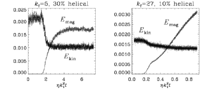
Figure 18: Evolution of kinetic and magnetic energies in two runs with fractional helicity. On the left hand panel, $k_{\rm f}=5$ and $\eta=2\times 10^{-3}$, whilst on the right hand panel, $k_{\rm f}=27$ and $\eta=2\times 10^{-4}$.

In Fig. 18 we show the results of two runs with fractional helicity forcing. In both cases the magnetic energy exceeds the kinetic energy by $k_{\rm f}/k_{\rm m}$ multiplied by an ‘efficiency factor’, $\epsilon_{\rm f}/\epsilon_{\rm m}$. In the first case we have $k_{\rm f}/k_{\rm m}=5$ and $\epsilon_{\rm f}/\epsilon_{\rm m}=0.3$, giving super-equipartition by about 1.5. This is roughly in agreement with Fig. 18. In the second case we have $k_{\rm f}/k_{\rm m}=27$ and $\epsilon_{\rm f}/\epsilon_{\rm m}=0.1$, giving super-equipartition by a factor of about 2.7. Although the run in the second panel of Fig. 18 has not been run for a full magnetic diffusion time (which is here ten times longer than in the first case), it seems clear that strong super-equipartition is still possible.

In the framework of $\alpha^{2}$ dynamo theory (Moffatt 1978, Krause & Rädler 1980), the large scale field is described by Eq. (36). In a periodic domain with minimum wavenumber $k_{1}$ the condition for large scale dynamo action is that the dynamo number, $C_{\alpha}=\alpha/(\eta_{\rm T}k_{1})$, exceeds unity. Standard estimates are $\alpha=-{\textstyle{1\over 3}}\tau\langle\mbox{\boldmath$\omega$}{}\cdot{\bf{u}}\rangle$ and $\eta_{\rm t}={\textstyle{1\over 3}}\tau\langle{\bf{u}}^{2}\rangle$ (e.g., Moffatt 1978), where $\tau$ is the correlation time. For strongly helical turbulence with forcing at a particular wavenumber $k_{\rm f}$, we have $|\langle\mbox{\boldmath$\omega$}{}\cdot{\bf{u}}\rangle|\approx\epsilon_{\rm f}k_{\rm f}\langle{\bf{u}}^{2}\rangle$, so

$$C_{\alpha}={|\alpha|/k_{1}\over\eta+\eta_{\rm t}}={|\alpha|/(\eta_{\rm t}k_{1})\over 1+R_{\rm m}^{-1}}=\epsilon_{\rm f}k_{\rm f}/\iota k_{1},$$ (86)

where $\iota=1+R_{\rm m}^{-1}$ is a correction factor involving the magnetic Reynolds number, defined here as $R_{\rm m}=\eta_{\rm t}/\eta$. For the Runs shown in Fig. 18, and with the numbers given in the previous paragraph, the values of $C_{\alpha}$ are 1.4 and 2.7, respectively. Thus, the dynamo number is supercritical. This is consistent with the clear growth of the large scale field seen in the simulations (Fig. 18). Maron & Blackman (2002) found that for $k_{\rm f}/k_{1}=5$ the critical value of $\epsilon_{\rm f}$ is around 0.5. This corresponds to $C_{\alpha}=2.5/\iota\approx 2$, which should still be supercritical. However, given that only modest resolution was used, the estimate for $\alpha$ may have been too optimistic.

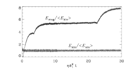
Figure 19: Evolution of kinetic and magnetic energies in a run with perfectly conducting boundaries in the $z$-direction. Note that the magnetic energy evolves in stages, similar to Fig. 6.

4.6 Fractional large scale magnetic helicity

We have seen that the large scale field strength will decrease if the small scale field is not fully helical. However, according to Eq. (85), the large scale magnetic field strength should increase if the large scale field were less helical. In order to demonstrate that this is true, we show in Fig. 19 the results of a run where the forcing is still 100% helical, but the large scale field is not fully helical. The latter has been achieved by adopting perfectly conducting boundary conditions, in which case it is no longer possible to have fully helical Beltrami waves. These calculations are otherwise similar to those presented in BD01, where the effects of nonperiodic boundary conditions was considered.

In Fig. 19 we see another remarkable feature that was already seen in Fig. 6: the large scale magnetic energy grows in stages. Indeed, looking at the actual magnetic field pattern one sees that the number of nodes in plots of the mean field decreases with time, just like in Fig. 6.

4.7 Position of the secondary peak

In the original Run 6 of B01 there was a field of intermediate scale that grew fastest at $k=7$. This wavenumber was found to be in agreement with $k_{\max}=|\alpha|/(2\eta_{\rm T})$, which is what one expects for an $\alpha^{2}$ dynamo. Here $\eta_{\rm T}=\eta+\eta_{\rm t}$ is the sum of microscopic and turbulent magnetic diffusivity and $\alpha$ represents the $\alpha$ effect that is caused by the helical small scale velocity. In the simulation, the only parameter that can be changed to make $|\alpha|/(2\eta_{\rm T})$ vary is the microscopic magnetic Reynolds number. In order to check our prediction regarding $k_{\max}$, we reduce the value of $\eta$ from $\eta=10^{-3}$ (as in B01) to $\eta=2\times 10^{-4}$. We find that now the fastest growing mode is at $k_{\max}\approx 15$, which is, on a logarithmic scale, almost indistinguishable from the forcing wavenumber, $k_{\rm f}=30$; see Fig. 20. At larger scales, $k<7$, the exponential growth is equally fast in all modes, independent of the (microscopic) value of $\eta$.

Figure 20: Scale separation in runs with different resistivity (first and second panel). Higher resistivity results in larger scale separation (third panel).

The reason for decreasing scale separation with increasing value of $R_{\rm m}$ is relatively easy to see. According to the dispersion relation for the $\alpha^{2}$ dynamo in an infinite domain (e.g., Moffatt 1978) the wavenumber of the fastest growing mode is

$$k_{\max}=|\alpha|/2\eta_{\rm T}=|\alpha|/2\iota\eta_{\rm t}=\epsilon_{\rm f}k_{\rm f}/2\iota.$$ (87)

So, unless $R_{\rm m}$ is small, in which case $\iota=1+R_{\rm m}^{-1}$ can be large, $k_{\max}$ will be around $k_{\rm f}/2$ giving a scale separation of 1:2. However, for small values of $\epsilon_{\rm f}$, the scale separation can be much larger.

In the high $R_{\rm m}$ limit, a scale separation of just a factor of 2 is hardly visible during the kinematic evolution of the field at that scale. Once the dynamo is in the nonlinear regime, i.e. once the small scale field has saturated, $\alpha$ will be quenched and $k_{\max}$ must decrease further.

In order to see that the sign of the magnetic helicity is indeed different at small and large scales we split the field into right and left handed parts, ${\bf{B}}={\bf{B}}^{+}+{\bf{B}}^{-}$ (see Sect. 2.2 and Christensson, Hindmarsh, & Brandenburg 2001), and show in Fig. 21 the magnetic energy spectra of ${\bf{B}}^{+}$ and ${\bf{B}}^{-}$, $M_{k}^{+}$ and $M_{k}^{-}$, respectively. Inverse transfer is only seen in the $M_{k}^{-}$ spectrum; the $M_{k}^{+}$ spectrum is dominated by the forcing scale.

Figure 21: Decomposition of magnetic field into positive and negative helical parts. Note that the magnetic energy at the forcing scale has increased between $t=250$ and $t=350$. The magnetic energy at large scales is dominated by helicity with negative sign (dashed curves).

5 Dynamos with shear

5.1 Evidence for magnetic Reynolds number dependence

Finally, we turn attention to the case of dynamos with shear. The presence of shear allows for an additional induction effect that is responsible for producing strong toroidal field from a poloidal (cross-stream) field component. According to a result from mean-field theory such dynamos can possess oscillatory solutions (e.g. Parker 1979). In a recent study by Brandenburg, Bigazzi, & Subramanian (2001, hereafter BBS01), where a velocity shear of the form $u_{y}(x)\propto\sin x$ was applied to helically driven turbulence in a periodic box, oscillatory solutions were confirmed also for non-mean field dynamos. The outstanding question, however, is whether the resistive time scale, which is now known to affect the saturation phase of the dynamo (B01, BBS01), also affects the cycle period. This question could not be answered conclusively in BBS01, because only one run with one value of the magnetic Reynolds number was considered.

In the meantime we have accumulated data from another run that had twice the value of the magnetic Reynolds number. The flow is driven by a forcing, which consist of two components: a term varying sinusoidally in the $x$-direction with wavenumber $k=1$ driving the shear and a term consisting of random Beltrami waves with wavenumber $k_{\rm f}=5$. As in BBS01, the ratio of the magnitudes of the two components of the forcing function is about 1:100, resulting in a shear velocity that is in the final state about 50 times larger than the poloidal rms velocity of the turbulence. This is large enough so that we can expect to be in the so-called ‘$\alpha\Omega$ regime’ where oscillatory solutions are the rule.

Corresponding butterfly diagrams of the toroidally averaged toroidal field components are shown in Fig. 22. The two diagrams are for two different $x$-positions, $x=\mp\pi$ and at $x=0$, where the shear $S={\rm d}{}u_{y}^{(0)}/{\rm d}{}x$ takes on its negative and positive extremum, respectively. The simulation was restarted from the run of BBS01 at the time $t=6\,000$ and run until $t=13\,000$ with $\eta$ reduced by a factor of $2.5$ with respect to BBS01. It turns out that the resulting magnetic field suffers a major disturbance after the magnetic diffusivity is reduced by just a factor of 2. More importantly, a clear pattern of a migratory dynamo wave is now almost absent. Instead, the toroidal flux pattern appears to just wobble up and down in the $z$ direction.

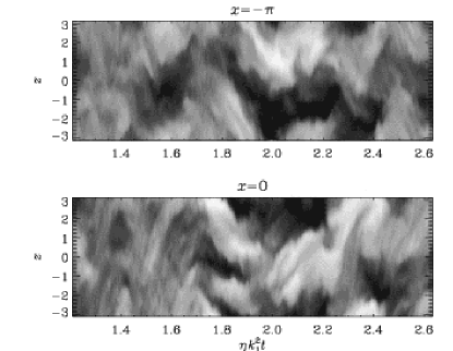
Figure 22: Butterfly diagram of ${\overline{B}}_{y}$, continuation from the run of BBS01, but with $\eta=2\times 10^{-4}$. Run (iii) of Table LABEL:Tao2.

One possible explanation for this result is that the dynamo wave was just very close to the threshold between oscillatory and nonoscillatory behaviour. This is not very likely however: the estimates of BBS01 indicated that the dynamo numbers based on shear, $C_{\Omega}=S/(\eta_{\rm T}k_{1}^{2})$, is between 40 and 80, whilst the total dynamo number (${\cal D}=C_{\alpha}C_{\Omega}$) is between 10 and 20 (see BBS01), and hence $C_{\alpha}=\alpha/(\eta_{\rm T}k_{1})\approx 0.25$. Thus, shear dominates strongly over the $\alpha$-effect ($C_{\Omega}/C_{\alpha}$ is between 150 and 300), which is typical for $\alpha\Omega$-type behaviour (i.e. oscillations) rather than $\alpha^{2}$-type behaviour which would start when $C_{\Omega}/C_{\alpha}$ is below about 10 (e.g. Roberts & Stix 1972).

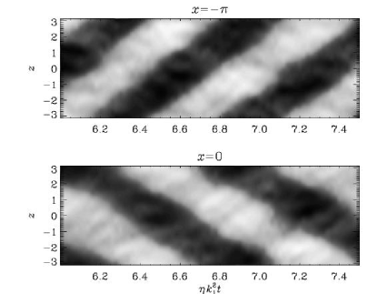
Figure 23: Butterfly diagram of ${\overline{B}}_{y}$, continuation from the run of BBS01, but with $\eta=10^{-3}$ (five times larger than in Fig. 22). Run (i) of Table LABEL:Tao2.

Another possibility is that an oscillatory and migratory dynamo is still possible, but it takes longer for the system to settle onto this solution. Unfortunately the present simulations have become prohibitively expensive in terms of computer time that this run cannot be prolonged by much further at this time. Instead, we have calculated a model with larger magnetic diffusivity and found cycle periods that are now somewhat shorter than before ($700...800$ compared to $1000...2000$ in BBS02), but in diffusive units they are similar ($0.7...0.8$ compared to $0.5...1.0$ in BBS02); see Fig. 23. This suggests that the period in this oscillatory dynamo is still controlled by the microscopic magnetic diffusivity. A more detailed comparison of various parameters with the other run presented above and with that of BBS01 is given in Table LABEL:Tao2.

Table 5: Summary of the main properties of the three-dimensional simulations with shear. Here, $\eta/(c_{\rm s}k_{1})$ is the magnetic diffusivity in units of the sounds speed and the wavenumber of the domain, and $\omega_{\rm cyc}=2\pi/T_{\rm cyc}$ is the cycle frequency. In Run (iii) there is no clear cycle visible.

Run (i) (ii) (iii) $\eta/(c_{\rm s}k_{1})$ $10^{-3}$ $5\times 10^{-4}$ $2\times 10^{-4}$ $\nu/\eta$ 5 10 25 $\langle{\bf{u}}^{2}\rangle^{1/2}/(\eta k_{1})$ 30 80 200 $\langle\overline{\bf{U}}^{2}\rangle^{1/2}/(\eta k_{1})$ 600 1200 2500 $\langle{\bf{b}}^{2}\rangle/B_{\rm eq}^{2}$ 4 6 20 $\langle\overline{\bf{B}}^{2}\rangle/B_{\rm eq}^{2}$ 20 30 60 $(\langle{\overline{B}}_{x}^{2}\rangle/\langle{\overline{B}}_{y}^{2}\rangle)^{1/2}$ 0.018 0.014 0.008 $\mu_{0}\langle\overline{\bf{J}}\cdot\overline{\bf{B}}\rangle/\langle\overline{\bf{B}}^{2}\rangle$ 0.11 0.06 0.014 $\omega_{\rm cyc}/(\eta k_{1}^{2})$ 8…9 6…12 $\geq 10?$

5.2 Can magnetic helicity ride with the dynamo wave?

We now want to address the question whether magnetic helicity can vary in space and time such that it is actually unchanged in the frame of the dynamo wave as it propagates. The background of these suggestions is as follows. Although the sign of the magnetic helicity in each hemisphere remains the same (and is opposite in the other hemisphere), its value still changes somewhat as the cycle proceeds. It is conceivable that even a small fractional variation may prove incompatible with the Parker-type migratory dynamo operating on a dynamical time scale. One possibility worth checking is that the magnetic helicity pattern could propagate together with the dynamo wave. In that case the magnetic helicity would be conserved in a Lagrangian frame moving with the wave, but not in an Eulerian frame. If this transport is due to advection, we would then expect systematic sign changes of $u_{z}$ in a space-time diagram, which does not seem to be the case however; see Fig. 24.

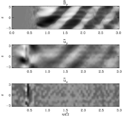
Figure 24: Butterfly diagram of ${\overline{B}}_{y}$ for the run of BBS01 with $\eta=5\times 10^{-4}$, compared with the corresponding diagrams of ${\overline{u}}_{y}$ and ${\overline{u}}_{z}$ for the same time interval. Note the presence of a ‘torsional’ oscillation in ${\overline{u}}_{y}$, i.e. a superposition of the driven shear flow (second panel), but the absence of any similar pattern in ${\overline{u}}_{z}$ (last panel). Run (ii) of Table LABEL:Tao2.

What does seem interesting, however, is the presence of what is usually (in the context of solar physics) referred to as a ‘torsional’ oscillation (Howard & LaBonte 1980). The toroidal flow pattern clearly traces the toroidal magnetic field pattern. More recently Howe et al. (2000) found another shorter period of 1.5 years which has been seen in helioseismological data. If this can indeed also be interpreted as the result of a similar magnetic field pattern (which is as yet undetected) then this would suggest the presence of multiple periods in the solar dynamo wave (cf. Covas, Tavakol, & Moss 2001).

In the discussion above we had mainly bulk motions in mind that would result in a transport of magnetic helicity. This does not need to be the case because magnetic helicity can also be transported along twisting magnetic field lines. This was used in the approach by Vishniac & Cho (2001), who proposed a dynamo effect based on a non-vanishing divergence of the magnetic helicity flux. If magnetic helicity were to ride with the dynamo wave, then this could perhaps correspond to the anticipated magnetic helicity flux. Unfortunately, in the parameter regime currently accessible to simulations the effect proposed by Vishniac & Cho has not yet been confirmed (Arlt & Brandenburg 2001). We may therefore conclude that transport or advection of magnetic helicity by meridional flows remains a possibility, but has not as yet been verified numerically.

5.3 Helicity loss in the presence of surface shear

The calculations of BD01 had the shortcoming that large scale shear was absent. Of course, shear does not produce net magnetic helicity, but it can lead to a spatial separation which could be particularly useful if there are surfaces. Large scale shear in the equatorial plane would wind up a poloidal field and hence would lead to magnetic helicity of opposite sign in the northern and southern hemispheres. In helically forced turbulence simulations, the various effects have only been studied in isolation: shear and helicity in BBS01, surface shear but no helicity in Arlt & Brandenburg (2001), and different helicities in the northern and southern hemispheres in Brandenburg (2001b).

Surface shear may allow for the direct production and transport of magnetic helicity of different signs in the two hemispheres on a dynamical time scale. Consider a differentially rotating star permeated by an initially uniform magnetic field parallel to the rotation axis. The differential rotation will wind up the magnetic field in different directions in the two hemispheres, where the field lines describe oppositely oriented screws. Such additional production and transport of magnetic helicity on a dynamical time scale may be important for the magnetic helicity problem. On the other hand, for this idea to be relevant we have to have a pre-existing large scale poloidal magnetic field, so this issue does not seem to address the problem of resistively limited field saturation.

In order to find out whether large scale surface shear is important we have considered a model similar to Run C2 of Arlt & Brandenburg (2001), i.e. with finite shear in a layer of thickness $2\pi$ and a quiescent (non-turbulent) halo with no shear outside. As before, the shear is given by $u_{y}(x)$, while the boundary to the halo is at $z=\pm\pi$. However, in contrast to the nonhelical calculations of Arlt & Brandenburg, we have now included a helical forcing that is negative (positive) above (below) the midplane. The results are in many respects similar to the runs of BD01 with a halo: around the time of saturation there is a strong negative burst of small scale magnetic helicity together with positive small scale current helicity. The resulting magnetic helicity fluxes both out of the turbulent domain as well as upwards on the two boundaries are fluctuating about zero. Thus, the addition of shear to the halo runs of BD01 seems to have only little effect on the evolution of helicity fluxes.

The evolution of the magnetic and kinetic energies is shown in Fig. 25. After about 0.08 resistive times the dynamo has entered the saturation phase which is then completed after 0.15 resistive times altogether. This is now much faster than in the case of periodic boundaries. Fig. 26 shows images of the mean toroidal magnetic field. Especially near the lower boundary of the disc surface (dash-dotted line) one sees the ejection of magnetic structures.

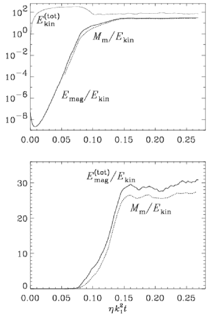
Figure 25: Semi-logarithmic and double-linear plots showing the evolution of kinetic and magnetic energies (dotted and solid lines), compared with the magnetic energy of the azimuthally averaged mean field. All quantities are normalised by the kinetic energy of the cross-stream motions. $E_{\rm kin}^{\rm(tot)}$ refers to the total kinetic energy including the shear. The ratio of the kinematic growth rate to the resistive time at large scales is here $\lambda/\eta k_{1}^{2}=160$.

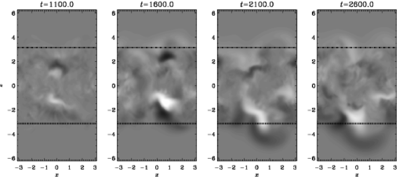
Figure 26: Loss of magnetic field through the upper and lower boundaries. Images of the mean toroidal field are shown at different times. Shear is positive (negative) at $x=0$ ($x=\pm\pi$). $\eta=10^{-4}$ and $\nu=5\times 10^{-3}$. The lines at $z=\pm\pi$ mark the boundaries of the turbulent slab.

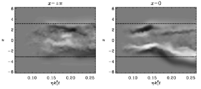
Figure 27: Butterfly diagram of the mean toroidal field of Fig. 26 at $x=\pm\pi$ and $x=0$. The lines at $z=\pm\pi$ mark the boundaries of the turbulent slab.

As can be seen in Fig. 27, the magnetic field structure is markedly different at $x=\pm\pi$ compared to $x\approx 0$, where it is stronger and pushed to the disc boundaries. This field expulsion to the boundaries could well be the result of usual field migration that is expected in the presence of shear and helicity. In terms of mean-field theory with positive $\alpha$ in the upper disc plane and negative below, we expect field propagation away from (towards) the midplane when shear is positive (negative). This is indeed consistent with our model where shear is positive (negative) at $x=0$ ($x=\pm\pi$).

6 Conclusions

In an attempt to clarify the problem of resistive versus dynamical time scales in models of the solar dynamo cycle we have tied up a number of loose ends that had been left open after the first exploratory simulations of B01, BD01, and BBS01. There are two distinct issues that may or may not be controlled by the resistive time: the time it takes for the large scale field to reach saturation and, once saturation is reached, the time scale on which the the large scale field can undergo cyclic variations as seen in the sun.

Looking back at Fig. 1 in the introduction we can still expect various approaches to be successful, although many others now seem to have been eliminated. One possibility was that the dynamo may still operate on a fast time scale if, like in the kinematic case, the wavelength of the dynamo wave is shorter than the extent of the system, and possibly only somewhat larger than the scale of the forcing. The main problem would then be to keep the process fast and to prevent the dynamo from developing scales as large as the box size. How this may happen in reality is not clear. It may well be connected to the geometry of astrophysical dynamos which have spherical or disc geometry and are not box-like. This corresponds to Alternative A in Fig. 1. The argument against this possibility is that even at intermediate scales the evolution towards larger scales (i.e. the motion of the secondary bump in the spectrum, cf. Figs 10 and 11) seems to occur on a resistive time scale. This can be seen from the reduction of the speed of the spectral bump, $\alpha_{\rm trav}$, as the resistivity is reduced (Table LABEL:Tsum). So the forcing scale may have to be not much smaller than the scale of the dynamo wave. Other plausible mechanisms could be based on non-$\alpha$ effect dynamos. Examples are negative magnetic diffusivity effects (cf. Zheligovsky et al. 2001), the incoherent $\alpha$-effect (Vishniac & Brandenburg 1997), and the Vishniac–Cho effect (Vishniac & Cho 2001). These are all subsumed under Alternative B in Fig. 1.

The remaining alternatives are all based on conventional $\alpha$ effect dynamos, so they have finite net magnetic helicity (although of opposite sign in the two hemispheres). In order for the dynamo to operate fast enough, resistive magnetic reconnection (with magnetic helicity destruction) has to be fast enough. This could only be the case near the surface where the microscopic magnetic diffusivity is sufficiently large. This corresponds to Alternative C in Fig. 1.

The other possibility is that the dynamo may work through losses of magnetic helicity of opposite sign, possibly at intermediate scales, for example near the surface (e.g. in coronal mass ejections and active regions) or across the equator. This is referred to as Alternative D. The simulations presented in Sect. 4.3 have shown that this is in principle possible. The problem here is that, so far, none of these mechanisms have been seen to occur naturally in any of the simulations investigated so far. It is therefore important to move toward more realistic simulations, perhaps in spherical geometry, with strong vertical stratification which could contribute to keeping the large scale field within the convection zone via turbulent pumping, but allowing fields above a certain threshold to escape through the surface.

The purpose of this review was to outline the present status of our understanding of nonlinear large scale dynamos. Things are developing rapidly with new simulations appearing every month. So far it has mainly been a process of elimination, because many different ideas have been around, and constantly more ideas are appearing. The least explored case is that of dynamos in realistic spherical geometries.

Although a number of direct simulations of MHD turbulence in spherical geometry have been analysed (Gilman 1983, Glatzmaier 1985, Glatzmaier & Roberts 1995, Drecker, Rüdiger & Hollerbach 2000, Ishihara & Kida 2000) the issue of fast versus resistively limited growth has not yet been investigated. This is indeed not an easy task. In order to distinguish between the two possibilities, one would need to verify explicitly whether a large scale field is generated on resistive times, or on a time scale that is independent of and much shorter than the resistive time scale. In addition, if the models show cyclic variability (which is desirable for solar dynamo models), the cycle length needs to be (asymptotically) independent of the resistive time if the dynamo is fast. One reason why such numerical experiments are difficult is that only at relatively large magnetic Reynolds numbers (which require high numerical resolution) the resistive time scale becomes sufficiently long so that it can clearly be distinguished from the dynamical time scale. A relevant dynamical time scale is the ratio $\lambda/(\eta k_{1}^{2})$ which has to exceed a value of around 20–30 before one can see that resistively limited growth or cycle periods have occurred (see B01). At the same time the resolution must not be too high because otherwise one may not be able to run the simulations for long enough before any large scale field has occurred. The same is true of hyperresistivity which tends to make the large scale resistive time scale extremely long so that nothing can be said about resistively limited growth. This explains why the issue of resistively limited growth is not yet well understood in more realistic geometries. Nevertheless, it would be worthwhile reanalysing data from recent, high-resolution dynamo simulations in the light of resistive limitations on the duration of the saturation phase and, if applicable, the cycle period.

Id: paper.tex,v 1.129 2002/04/30 17:52:49 brandenb Exp