Dynamical Masses of Young Star Clusters in NGC 4038/4039

Abstract

In order to estimate the masses of the compact, young star clusters in the merging galaxy pair, NGC 4038/4039 (“the Antennae”), we have obtained medium and high resolution spectroscopy using ISAAC on VLT-UT1 and UVES on VLT-UT2 of five such clusters. The velocity dispersions were estimated using the stellar absorption features of CO at 2.29 $\mu$m and metal absorption lines at around 8500 Å, including lines of the Calcium Triplet. The size scales and light profiles were measured from HST images. From these data and assuming Virial equilibrium, we estimated the masses of five clusters. The resulting masses range from 6.5 $\times$ 10⁵ to 4.7 $\times$ 10⁶ M_☉. These masses are large, factor of a few to more than 10 larger than the typical mass of a globular cluster in the Milky Way. The mass-to-light ratios for these clusters in the V- and K-bands in comparison with stellar synthesis models suggest that to first order the IMF slopes are approximately consistent with Salpeter for a mass range of 0.1 to 100 M_☉. However, the clusters show a significant range of possible IMF slopes or lower mass cut-offs and that these variations may correlate with the interstellar environment of the cluster. Comparison with the results of Fokker-Planck simulations of compact clusters with properties similar to the clusters studied here, suggest that they are likely to be long-lived and may lose a substantial fraction of their total mass. This mass loss would make the star clusters obtain masses which are comparable to the typical mass of a globular cluster.

1 Introduction

During the last years, many interacting and merging galaxies were discovered to host large numbers of young star clusters which formed during the merging process (Holtzman et al. (1992); Whitmore et al. (1993); Meurer et al. (1995); Whitmore et al. (1997, 1999); Zepf et al. (1999)). The overall properties of these clusters suggest that they could be the progenitors of the globular cluster populations seen in normal nearby elliptical and spiral galaxies (e.g., Zepf & Ashman (1993)). Such an hypothesis also has the attractive implication that if ellipticals formed through the merger of two large spiral galaxies (as suggested in the popular hierarchical merging model of galaxy formation e.g., Kauffmann, White, and Guiderdoni (1993)), these young clusters might evolve into the red (supposedly metal rich) part of the globular cluster population of elliptical galaxies when the merger is complete (e.g. Schweizer (2001)). However, this hypothesis needs to be tested by determining the characteristics of both, individual young clusters and the cluster population as a whole.

Globular clusters have a typical mass of 1-2$\times$10⁵ M_☉ and a mass function which is log-normal (e.g., Harris (1991)). The population of clusters in NGC 4038/4039 (“the Antennae”), however, has a power law luminosity function, and the same shape is also suggested for the mass function (Whitmore et al. (1999); Zhang & Fall (1999)). Masses determined from photometric data are as large as a few $\times$10⁶ M_☉ for some of the clusters (Zhang & Fall (1999); Mengel et al. (2001)) and the determined ages span a large range (Whitmore et al. (1999); Mengel et al. (2001)).

At first glance, the population of globular clusters in the Milky Way and those in the Antennae seem to have vastly different ensemble characteristics. For example, the most massive clusters in the Antennae are at least a factor of few more massive than those in the Milky Way. However, given the large number of clusters formed in the Antennae, it seems reasonable that the mass function is sampled up to a high upper mass, and moreover mass loss during the evolution of the young clusters can be expected to play a role. Evolution over a Hubble time might convert the power law cluster mass function into a log-normal one, if lower mass clusters were dissolved preferentially during the evolution. Dynamical models like those, for example, of Chernoff & Weinberg (1990) and Takahashi & Portegies Zwart (2000) provide theoretical support for the necessary differential evolution from a power-law mass distribution function into a log-normal distribution.

Dynamical cluster masses are less model dependent than those determined from photometry only, or, at the very least, have a different set of dependencies. The dynamical mass is derived from the stellar velocity dispersion in combination with the cluster size and light profile. While the photometric mass estimates depend on the model assumed for the star formation parameters (time-scale, age, IMF slope, lower and upper limiting masses, metallicity, etc), the dynamical mass estimates rely only on the validity of the Virial equilibrium (i.e., the potential is due to the collective gravitational effects of individual stars – self-gravitating – and is changing only slowly with time), and the assumed constancy of the M/L ratio within the cluster. The comparison of photometric and dynamical cluster masses (cluster M/L) constrains the slope of the mass function and may reveal the presence or absence of low mass stars. The fraction of low mass stars influences the survival probability of the cluster during a few Gyrs of evolution, as clusters rich in low-mass stars are less prone to destruction (e.g., Takahashi & Portegies Zwart 2000).

More specifically, we have used high spectral resolution spectroscopy conducted at the ESO VLT to estimate the stellar radial velocity dispersion $\sigma$, and high spatial resolution imaging from archival HST images (Whitmore et al. (1999)) to estimate the size scales (e.g., the projected half-light radius r_hp). This results in M_dyn for individual clusters which can be estimated using the equation:

$$M=\frac{\eta\sigma^{2}r_{hp}}{G}$$ (1)

Where $\eta$ is a constant that depends on the distribution of the stellar density with radius, the mass-to-light ratio as a function of radius, etc. The only assumption that goes into Virial relations of this form is that the cluster is self-gravitating and is roughly in equilibrium over many crossing times (i.e., it is not rapidly collapsing or expanding). The calculations of Spitzer (1987) indicate that for a wide range of models, $\eta$ $\approx$ 10. Under the assumption of isotropic orbits, $\eta$ differs from 3 (the pure Virial assumption) since the “gravitational radius” must be scaled to the projected half-light radius (or some measurable scale) and because the measurement of the velocity dispersion is not the central velocity dispersion but is a measurement which is weighted by the light profile. So differing mass profiles have different values of $\eta$ appropriate for estimating their dynamical masses. For example, globular clusters in the Milky Way exhibit a range of concentration parameters (logarithm of the ratio of the tidal radius to the core radius) in a King model (King 1966) of approximately 0.5 to 2.5 (e.g., Harris 1991). Over this range of concentrations, $\eta$ varies from about 9.7 to 5.6. Hence, accurately measuring the light profiles (and of course the assumption that the light profile traces the mass profile) is crucial in estimating the masses.

Recent attempts at estimating the dynamical masses of similar clusters in other galaxies has met with some success. Notably, Ho & Filippenko 1996a and Ho & Filippenko 1996b were able to estimate the masses of two luminous young star clusters in the blue compact dwarf starburst galaxy NGC 1705 (1705-1) and NGC 1569 (1569A). They measured velocity dispersions for 1705-1 and 1569A of 11.4 km s^-1 and 15.7 km s^-1 respectively. Under the assumption that $\eta$ = 10, Sternberg (1998) estimated that these clusters have masses of about 2.7 $\times$ 10⁵ M_☉ for 1705-1 and 1.1 $\times$ 10⁶ M_☉ for 1569A. More recently, Smith & Gallagher (2001) have estimated the dynamical mass of the luminous star-cluster in M82, M82-F. Assuming $\eta$=10, they find a mass of 1.2$\pm$0.1$\times$ 10⁶ M_☉. This mass estimate implies that the mass-to-light ratio of M82-F is very extreme and requires either a very flat mass function slope or a lack of low mass stars for a Salpeter-like mass function slope. Interestingly, this small sample of clusters seems to require a range of IMFs to explain their mass-to-light ratios.

The purpose of the present paper is to derive masses for a small sample of young compact clusters in the Antennae galaxies - the nearest merger - and to use these mass estimates to constrain the functional form of the IMF in these clusters. Since it is important that the velocity dispersion be determined from the stellar component of the cluster, we have undertaken a program to observe extinguished clusters in the K-band, to take advantage of the strong CO absorption band-heads beyond 2.29 $\mu$m, and unextinguished clusters in the optical, to take advantage of the strong absorption of the Calcium Triplet (CaT) and other metal lines around 8500Å. These features are strong in atmospheres of red supergiants which would be expected in large numbers in clusters with young ages ($\approx$6-50 Myrs) and thus particularly well-suited for estimating the masses of clusters like those in the Antennae. Given that previous investigators (e.g., Ho & Filippenko 1996a ; Ho & Filippenko 1996b ) have measured velocity dispersions around 15 km s^-1 suggests that to conduct such measurements would require a minimum resolution of R$\approx$9000. Such resolutions are now available using ISAAC on VLT-UT1 which with its narrowest slit delivers R$\approx$9000 and UVES on VLT-UT2 which delivers a resolution of $\approx$38,000 with a 1″ wide slit.

2 Observations

2.1 Moderate Spectral Resolution K-band Spectroscopy

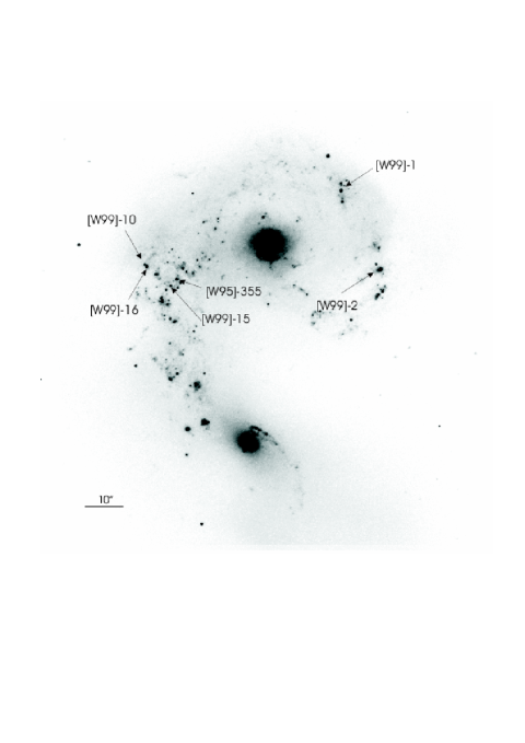
Figure 1: ISAAC Ks-band image of NGC 4038/4039 (taken during a run in April 2001) with labeling of the clusters that were observed using ISAAC and UVES spectroscopy

Spectroscopy in the K-band was performed with ISAAC at VLT-UT1 on April 17 2000. The spectrograph was configured to have a 0$\aas@@fstack{\prime\prime}$3 slit and the medium resolution grating was tilted such that the central wavelength was 2.31$\mu$m with a total wavelength coverage from 2.25 to 2.37$\mu$m. This was sufficient to include the ¹²CO (2-0) and (3-1) absorption bands and at a resolution ($\lambda/\Delta\lambda$) of about 9000. Observations of late-type supergiant stars were taken so that they could be used as templates for the determination of the velocity dispersions. Various templates were observed, however, due to incorrect classifications in the literature, only one of them actually was an M-type supergiant. More template stars were observed by Linda Tacconi during an observing run on August 15 2000 using the same instrumental set-up. Observations were performed by nodding along the slit and dithering the source position from one exposure to the next. Atmospheric calibrator stars were observed several times during the night.

The target clusters were selected using the results from NTT-SOFI imaging observations performed in May 1999 (Mengel, Ph. D. Thesis, der Ludwig-Maximilians-Universität München, 2001; Mengel et al. 2001, in preparation). They included narrow band imaging in the CO(2-0) band-head and revealed those clusters which are at an age where the near-infrared emission is dominated by red supergiants. The clusters with the highest equivalent width in the CO band-heads, highest luminosity, and high extinction were selected as the ISAAC targets (for the location of all observed clusters see Fig. 1). Two target clusters were positioned in the first slit position. These were two clusters with a separation of $\sim 5$″ located in the region where the galaxy discs apparently overlap (“the overlap region”). One of them has an optical counterpart, [W99]15, the other one is detectable only in the I-band, therefore denoted as a “Very Red Object (VRO)” by Whitmore & Schweizer (1995) (with the designation: [WS95]355). Their detectability in at least one band from the HST imaging program of Whitmore et al. (1999) was a necessary additional constraint, since the compactness of each cluster means that their radii must be measured from HST data (see §3.4). The second slit position included only one bright cluster ([W99]2), which has a relatively low extinction and was also observed with UVES. Due to the extreme narrowness of the slit, object drifts made several re-acquisitions necessary, especially when the object was transiting. The ISAAC observations are summarized in Table 2.

Table 1: Summary of ISAAC spectroscopy. The first slit position included two clusters, the second one cluster. The supergiants were observed to provide template spectra for the determination of velocity dispersions. The slit width was 0$\aas@@fstack{\prime\prime}$3, resulting in a resolution R = $\lambda/\Delta\lambda$ of 9000. Seeing variations are expected to have no effect on the spectral resolution given the narrow slit width. The total integration time was split up into several integrations of duration T_int. The K-band magnitudes were determined from an ISAAC Ks-band image (aperture diameter 1$\aas@@fstack{\prime\prime}$74). The seeing value refers to an average for the monitored V-band seeing during the integration. The stars were observed during two observing runs (2000 and 2001), and those marked with LT were kindly observed by Linda Tacconi during another run, because the 2000 run had resulted in only one useful supergiant spectrum.

Position	Object	mV	mK	m${}_{K_{0}}$	Tint	Total ON time	Seeing	Comments
		[mag]	[mag]	[mag]	[s]	[s]
Slit 1	[W99]15	19.4	15.9	15.8	600	15600	0$\aas@@fstack{\prime\prime}$7	Difficulties keeping both
	[WS95]355	$\approx$22.1	15.7	15.4	600	15600		targets in slit during 2 integrations
Slit 2	[W99]2	17.0	14.0	14.0	600	2400s	0$\aas@@fstack{\prime\prime}$9

and the following stars: K5Ib (HD183589), K5Ib (HD53177, LT), M0I (CD-44 11324, LT),

M0-1Iab (HD 42475), M1I (BD+0 4030), M1Iab (HD 98817), M1Ib (HD 163755), M2Iab (SAO 15241),

M3Ia-Iab (HD103052), M3.5I (BD+13 1212), M5Iab (HD 142154)

2.2 High-Resolution Optical Spectroscopy

High-resolution optical echelle spectroscopy was performed using UVES at VLT-UT2 on the night of 18 April 2000. The instrument was configured with a slit width of 1″, which resulted in a resolution of R$\approx$38,000 (depends on wavelength). A dichroic was placed in the light path allowing the use of both the red and blue arms of the spectrograph. However, in this paper we will discuss only the results obtained with data from the red arm. The central wavelength of the red arm was shifted to 8400Å since part of the CaT (at NGC 4038/4039 redshift of z$\sim$0.005 located roughly at: 8540Å, 8585Å and 8705Å) would have fallen right in the small gap between the two CCDs that cover the lower and the upper part of the spectra in the red arm. The CCDs were read out with a binning of 2x2, 50kHz and high gain. For the cluster selection we applied the same criteria as for the clusters observed with ISAAC, however, for the UVES observations, we selected only those with relatively low optical extinction and bright I-band magnitudes. To boost the efficiency of the observing, we additionally required the clusters to have a nearby cluster within the slit of UVES (which is only 10″ due to the echelle design). The clusters observed were [W99]1 and [W99]43 in one slit position, [W99]10 and [W99]16 in a second slit position. Unfortunately, [W99]43 and [W99]10 turned out to be too faint to extract a spectrum of sufficient S/N for further analysis. A third slit position covered [W99]2, common to ISAAC and UVES. Obtaining two independent observations of [W99]2 provides an independent estimate of the velocity dispersion to test the uncertainties of our measurements and to gauge whether there might be some systematic differences in velocity dispersions determined from the CaT in the optical with UVES versus that obtained from the CO band-head with ISAAC in the near-IR. A range of template supergiants was observed (early K through late M-type supergiant stars), but also several hot main sequence stars (late O through mid B-type main sequence stars). Massive main sequence stars are expected to dominate the blue spectrum and to contribute significantly to the flux in the I-band (Bruzual & Charlot 1993). Due to the high dispersion and faint sky background, integration times could be very long and were only limited by the desire to keep the number of cosmic ray hits down to a reasonable limit. The UVES observations are summarized in Table 2.

Table 2: Summary of UVES spectroscopy of science targets (star clusters and template stars). The spectral resolution was R$\approx$38,000, and differences in the seeing for different objects had no measurable effect on the shape of the absorption features in the stellar spectra.

Position	Object	mV	mK	m${}_{K_{0}}$	Tint	Ttot	Seeing	Comments
		[mag]	[mag]	[mag]	[s]	[s]
Slit 1	[W99]1	17.6	14.7	14.7	4800s	9600s	0$\aas@@fstack{\prime\prime}$7	required pausing of integration
	[WS95]43	20.0			4800s	9600s		due to A.O. software crash
Slit 2	[W99]10	19.0	15.6	15.6	4800s+1800s	11400s	0$\aas@@fstack{\prime\prime}$85	required pausing of integration
	[W99]16	19.0	15.5	15.5	4800s+1800s	11400s		due to A.O. software crash
Slit 3	[W99]2	17.0	14.0	14.0	4600s	4600s	1$\aas@@fstack{\prime\prime}$2

And the following stars: M3Iab (HD 303250), M5I (HD 142154), M1Ib (HR 6693), MIa-Ib (HR 4064)

K7IIa (HD 181475), K5Ib (HR 7412), K5II (HR 7873), K3Ib-IICN (HR 6959), K3II (HR 6842)

K2.5IIb (HR 7604), K2II (HR 6498), K2Ib (BM Sco), K0.5IIb (HR 6392), K0Ia (HR 6392)

B5V (HR 5914), B5V (HR 5839), B2V (HR 6028), B2V (HR 6946) with integration times

between 1s and 20s, and some atmospheric and flux calibrators

3 Reduction and Analysis

3.1 Reduction of the near-IR data

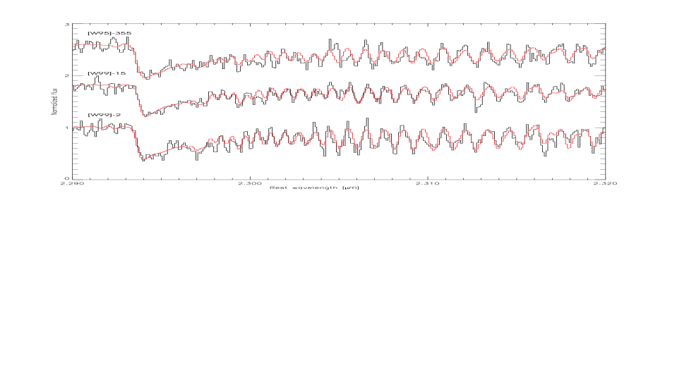
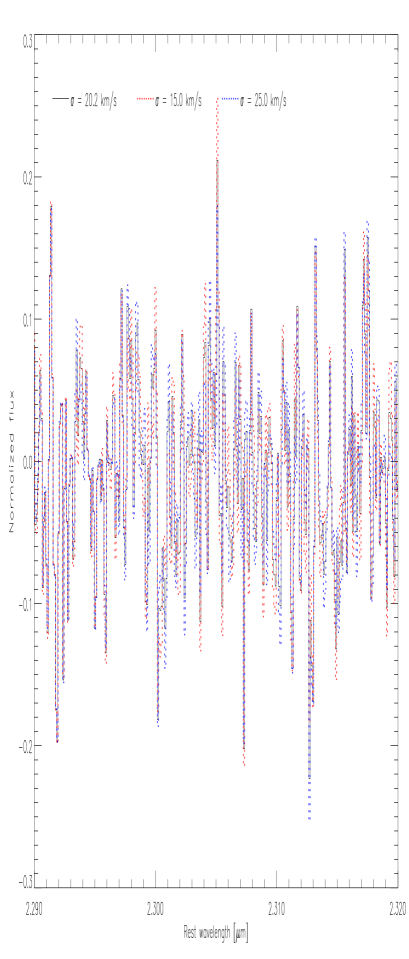
Figure 2: ISAAC Spectra of the three clusters [WS95]355, [W99]15 and [W99]2 (top to bottom, black) with best fits (grey). The bottom plot shows the residuals of the fit to spectrum [W99]15 for the best fit and for two fits with lower and higher velocity dispersions. This gives a visual impression of how much the velocity dispersion affects the spectral features.

The reduction of ISAAC data was performed in a standard way using the IRAF data reduction package. The reduction included dark subtraction and flat-fielding (using a normalized flat-field created from dome flat observations) on the two-dimensional array. Sky subtraction was performed pairwise, followed by a rejection of cosmic ray hits and bad pixels. The spectra were then corrected for tilt and slit curvature by tracing the peak of the stellar spatial profile along the dispersion direction and fitting a polynomial to the function of displacement versus wavelength. The corresponding procedure was also applied to the orthogonal direction. Single integrations were combined by shifting-and-adding, including a rejection of highest and lowest pixels. The rejection could not be applied to observations of [WS99]2, because they consisted of only a limited number of single frames. The object spectra were then extracted from user defined apertures. A linear fit to the background (below $\approx$7% of the peak intensity for all clusters) on both sides of the object spectrum was subtracted.

The spectra were wavelength calibrated using observations of arc discharge lamps. An atmospheric calibrator (B5V) was observed and reduced in the same way as the target and used to divide out the atmospheric absorption features from the spectra.

3.2 Reduction of the optical echelle data

Reduction of the UVES data was performed within the echelle spectra reduction environment of IRAF. Reduction included bias subtraction, flat-fielding and extracting the spectrum from user supplied apertures. A background is fit to neighboring regions and subtracted. Also here, the background was below $\approx$7% of the peak intensity for all clusters. This step includes a bad pixel rejection. The full moon was fairly close to the Antennae during the integrations, and its scattered light introduced a solar spectrum into the data. However, this contribution is very effectively removed during background subtraction.

Wavelength calibration required the identification of many lines in the ThAr-spectra for each of the echelle orders which were identified using a line table available from the ESO-UVES web pages. A dispersion function was then fit and applied to the object data. This data set contains each order of the spectrum in a separate channel. These separate channels are combined into one final spectrum covering the total wavelength range. This involves re-gridding of the wavelength axis into equidistant bins and averaging in the overlapping edges of the orders. The spectral resolution obtained is R$\approx$38,000 across all orders.

3.3 Estimating the Velocity Dispersions

For each spectrum (both the optical and near-IR spectra), we estimated the $\sigma$ of the broadening function (assumed to be a Gaussian) which best fit the cluster spectrum in the following way. The stellar spectrum (the template spectrum) was broadened with Gaussian functions of variable $\sigma$ in velocity space. The resulting set of spectra were then compared with the cluster spectrum. The best fit was determined by evaluating $\chi^{2}$ and then search for the minimum of the function $\chi^{2}$(v_r,$\sigma$) using a simplex downhill algorithm for the tour through parameter space.

3.3.1 Unique Character of the near-IR Estimates

Obviously, the template spectrum has to be a good overall match to the cluster spectrum, otherwise an erroneous velocity width will be derived for the cluster. For a star cluster that formed $\sim$10 Myrs ago, late K through early M supergiants are expected to provide the largest contribution to the flux at 2.3$\mu$m. However, according to population synthesis models (e.g., Leitherer et al. (1999), Sternberg (1998)), there will be a non-negligible contribution to the flux from hot main sequence stars. Since the stars are hot (O and B-type stars), this “diluting continuum” will be an essentially featureless continuum which solely decreases the equivalent width of the CO band-heads. This has the effect of shifting the apparent dominating stellar type towards higher effective temperatures. Starting out with a template spectrum with weak CO features leads to very low velocity dispersions, the opposite is the case if an M5I star (strong band-heads) is used, with vast differences in the results (a few km s^-1 to up to about 30 km s^-1).

To first order, the velocity dispersion determined from different stellar templates agrees if the CO equivalent widths match. This is achieved by adding a (positive or negative) continuum to the stellar spectrum, which dilutes or enhances the CO features.

To second order, there are two different indicators that can be used to constrain the matching stellar template. Both relate to the shape of the CO band-head, due to variations in that shape between the different supergiant spectral classes. The various rotational transitions are resolved in the ¹²CO(2-0) and the ¹²CO(3-1) band-head. We performed tests of our analysis technique by creating a simulated cluster spectrum with an input velocity dispersion $\sigma_{in}$, added noise (usually S/N = 15) and re-determined the velocity dispersion $\sigma_{out}$ using different template star spectra. With the correct template (out = in), we obtained in 30 test runs an average $\sigma_{out}$ = 14.7$\pm$0.7 km s^-1 (with $\sigma_{in}$ = 15.0 km s^-1). Performing the same test on an input spectrum that was diluted by a flat continuum (10%), but still fitting with the undiluted template, the velocity dispersion increased (17.9$\pm 1.7$ km s^-1), as expected. Fitting other stellar types (M0I, M1I) yields similar results. But the mismatch can be diagnosed by:

• determining $\sigma$ over several different wavelength ranges. With the matching template, $\sigma_{out}$ depends only weakly (maximum differences $\sim 6\%$) on the selected wavelength range, no matter if only the band-head, only the overtones, or both are covered. A template mismatch causes differences in the $\sigma_{out}$ for different wavelength ranges of $\sim 25\%$ typically, but sometimes more.

• inspecting the shape of the fit around the tip and the rising edge of the band-head, which provides a good match only for the correct template

3.3.2 Unique Character of the Optical Estimates

The determination of the velocity dispersion for the optical echelle data used the same procedure as for the ISAAC spectra, relying on the Calcium Triplet around 8500Å, but also using the Mg absorption feature at 8800Å and other weaker metal absorption lines between 8400 and 9000Å.

Examining the spectra in detail, it was obvious that they are composed of a mixture of light from supergiants and hot main sequence stars. This means that the spectra cannot be simply fit by broadening the stellar template, but that either the hot star contribution needs to be added to the template, as was done in the case of the ISAAC spectra, or that the contribution needs to be subtracted from the cluster spectrum.

Here, the procedure was different from that applied to ISAAC data, because the hot main sequence stars were not completely featureless over the analyzed wavelength range, but had some Paschen absorption features. Pa16, Pa15 and Pa13 lie slightly red-ward of the CaT wavelengths 8498Å, 8542Å, and 8662Å, respectively. Since the widths of these lines are mainly due to line broadening in the atmosphere and rotation of the star itself and only an insignificant fraction of the width is due to the velocity dispersion of the star cluster, they cannot be used to estimate the velocity dispersion. Therefore this weak contribution was subtracted from each cluster before the velocity dispersion was estimated. The amount of subtraction was estimated by the strengths of the Paschen line absorption and the appropriate template for the subtraction was chosen for its ability to remove the contribution accurately. Given the S/N of the spectra and the weakness of the features removed, the final characteristics of the subtracted spectrum were not very sensitive to the exact template used.

The cluster [W99]2 merits some specific discussion since it has both ISAAC and UVES observations and also some peculiarities were noted compared to the other clusters observed with UVES. Fig. 3 shows fits of an M3I spectrum to pieces of the spectrum of the cluster [W99]2. The latter had a 45% contribution of B2V stars subtracted. This contribution was determined by interactively subtracting the spectrum of the B2V star until the Paschen absorption features were reduced down to the noise level of the cluster spectrum. In addition, we fit the continuum of the cluster spectrum using a combination of a B2V and an M3I star spectrum, in which the relative contributions of the two template stars was the fit parameter. The best fitting combination again included a 45% contribution of B2V stars. Moreover, the relative contributions of M3I and B2V stars in I and K band agree with the determined contributions to the ISAAC and UVES spectra, respectively, for this cluster.

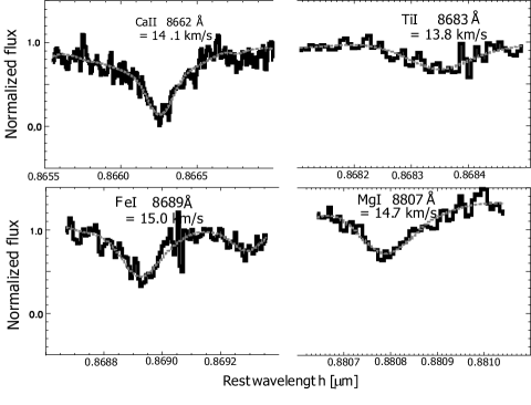
Figure 3: Displayed are parts of the normalized spectrum of cluster [W99]2 (black), together with the fit (red). The four pieces were fit separately, and the average value of the velocity dispersion is $\sigma$ = 14.2 km s^-1. It is worth noting that this is the cluster which was also observed with ISAAC, and to compare the results (see Figure 2).

3.4 Estimating the Sizes of the Observed Clusters

In order to make an estimate of the mass, it is necessary to have a measure of the cluster radius and profile shape. Whitmore et al. (1999) found that many of the young star clusters in images taken with the Wide Field Planetary Camera on HST (WFPC-2) of the Antennae were slightly-to-well-resolved and estimated their sizes. Their main aim was to determine the average radii of the clusters and to compare them to those observed in other galaxies, both to the young clusters in other mergers and to globular clusters. They found that the mean effective radius of the clusters in the Antennae is r_eff $\approx$ 4 pc. However, Whitmore et al. (1999) did not present their results on individual clusters. Brad Whitmore kindly provided us with their estimates of the effective radii for the clusters we observed with ISAAC and UVES. But given the importance of size and light profile to the mass determination, we additionally measured them ourselves from the HST I-band images.

Similar to what Whitmore et al. (1999) did to make such estimates we reduced archival HST I-band images (see Whitmore et al. 1999 for the details concerning the images) using the drizzle technique (see the Drizzle Handbook available from STScI). Given the pixel sizes of the HST chips (0$\aas@@fstack{\prime\prime}$101 pix^-1 for the Wide Field Camera arrays and 0$\aas@@fstack{\prime\prime}$045 pix^-1 for the Planetary Camera array), and the distance to NGC 4038/4039, which implies a scale of 93 pc arcsec^-1, the factor of two improvement in the sampling of the HST point-spread-function (PSF) due to drizzling the images is critical in getting a robust estimate of the sizes. At the typical cluster size, r${}_{eff}\approx$ 4 pc, the subtended scale is only 0$\aas@@fstack{\prime\prime}$043 or about one pixel of the Planetary Camera! For this analysis we used the ishape routine described by Larsen (1999) implemented in the BAOLAB data reduction package developed by Larsen. The ishape routines were especially designed to work more efficiently than typical deconvolution routines at determining the sizes of slightly extended objects. ishape convolves the user-provided PSF with the given cluster profile and determines the minimum $\chi^{2}$ for a range of sizes using a simplex downhill algorithm to find the minimum. The PSF we selected for this convolution is one from the Tiny Tim program (Krist 1995) which Whitmore et al. (1999) argue persuasively is appropriate for these data. We fit each cluster with a range of provided profiles which include Gaussian profiles, King profiles of several concentration parameters (King (1966)), and Moffat profiles of two different concentrations (Moffat 1967). The program produces a reduced $\chi^{2}$ to measure the significance of the fit and various images (artificial cluster image, the original input image, an image of the residuals between original and fit, and an image of the weights applied to each pixel) to judge the quality of the fit. The code also provides a handy weighting procedure that enables the rejection of “outliers” in the radial cluster profile, thereby excluding, for example, neighboring stars and/or clusters.

Table 3: The cluster masses as they were derived from the ISAAC and UVES spectra (in column “Inst.” indicated by I and U, respectively) in comparison with the supergiant template spectrum. The age was derived from the combination of W_Brγ, W_CO, and W_CaT. For cluster [W99]2, it agrees well with the age estimated from the UV spectrum of 7$\pm$1 Myrs Whitmore et al. (1999). The size is the projected half-light radius r_hp estimated as described in §3.4 (for the cluster marked with ^a, we could not obtain a satisfactory fit and used the value provided by B. Whitmore). W_CO was estimated from the ISAAC spectra between rest-frame wavelengths 2.2924$\mu$m and 2.2977$\mu$m, ([W99]2 also from 3D integral field spectroscopy), and W_CaT from the UVES spectra, according to the definition in Díaz et al. (1989). The stellar velocity dispersion $\sigma$ was determined as described in §3.3, for [W99]2 the average value of ISAAC and UVES measurements is given ($\sigma$=14.0$\pm 0.8$ and 14.3 $\pm 0.5$ km s^-1, respectively). M_vir is the Virial mass determined from equation 1 with the 1$\sigma$-uncertainties given in column $\sigma_{M}$ . The light-to-mass ratios were derived from the extinction corrected magnitudes and a distance modulus to NGC 4038/4039 of 31.41.

Cluster	Inst.	WCO	WCaT	Age	$\sigma$	rhp	log Mvir	$\sigma_{M}$	log LV/M	log LK/M
	I/U	[Å]	[Å]	[106yr]	[km/s]	[pc]	[M☉]	[%]	[L☉/M☉]	[L☉/M☉]
$[$WS95$]$355	I	16.3$\pm$0.2	-	8.5$\pm$0.3	21.4$\pm$0.7	4.8$\pm$0.5a	6.67	12	…	1.05
$[$W99$]$15	I	17.0$\pm$0.2	-	8.7$\pm$0.3	20.2$\pm$0.7	3.6$\pm$0.5	6.52	16	0.89	1.09
$[$W99$]$2	I/U	16.2$\pm$0.2	6.4$\pm$1.0	6.6$\pm$0.3	14.2$\pm$0.4	4.5$\pm$0.5	6.31	12	1.54	2.00
$[$W99$]$1	U	17.5$\pm$1	8.6$\pm$1.0	8.1 $\pm$0.5	9.1$\pm$0.6	3.6$\pm$0.5	5.81	19	1.76	2.22
$[$W99$]$16	U	19$\pm$4	9.9$\pm$1.0	10$\pm$2	15.8$\pm$1	6.0$\pm$0.5	6.51	15	0.50	1.20

4 Results

Our results are summarized in Table 3. We find a range of cluster velocity dispersions from about 9 km s^-1 to over 20 km s^-1. One concern about any such measurements is the reliability of the final results. For the optical echelle data, the instrumental resolution, $\sigma_{instrument}$=3.2 km s^-1 ensures that the cluster line profiles are always well-resolved. The situation for the near-IR data is less clear. For the clusters where the velocity dispersions were estimated from the near-IR CO band-head, the measured values are above or approximately at the instrumental resolution ($\sigma_{instrument}$=14.2 km s^-1) and are thus likely to be secure. However, we were worried about possible systematics effects that might influence the final estimates. To make an estimate of these possible problems, we constructed “test data” from the stellar templates that were artificially broadened and had noise added to mimic the real cluster data from both the ISAAC and UVES observations. This allowed us to investigate possible systematic problems in the way each of the data sets was analysed and allowed us to discover the most robust ways of analyzing the data. In addition, for one of the clusters, [W99]2, we obtained both UVES and ISAAC spectra of this cluster to observe any systematic differences between the two data sets that might lead us to conclude that there are systematic differences in the properties among the clusters.

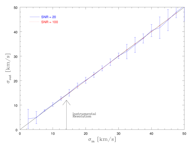
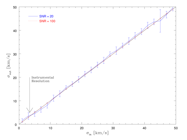
Figure 4: Artificial data with a S/N comparable to our data (S/N = 20) and with a S/N = 100 were created from stellar template spectra and the input velocity dispersion was redetermined. The average value of 30 test runs with the variance is displayed for both instruments (Top: ISAAC, Bottom: UVES).

From experiments with the test data, we found no systematic problems in the estimated dispersions as long as the template was a good match (as described earlier) and for velocity dispersions that were above approximately 50% of the instrumental resolution. We conducted these simulations for the range of S/N spanned by the data for the clusters (Figure 4). As a by product of these simulations, we were able to estimate the uncertainties in our estimates by conducting many (several tens) trials for each input broadening width. From the distribution of resulting dispersion estimates, we were able to determine the average output velocity dispersion to look for systematic offsets and the variance to provide a likelihood estimate of the uncertainty in any one measurement.

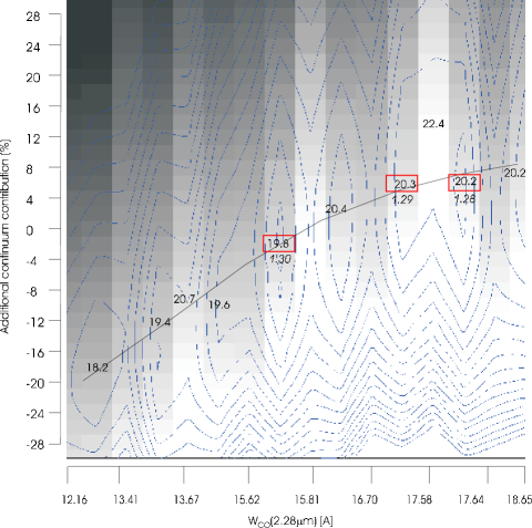
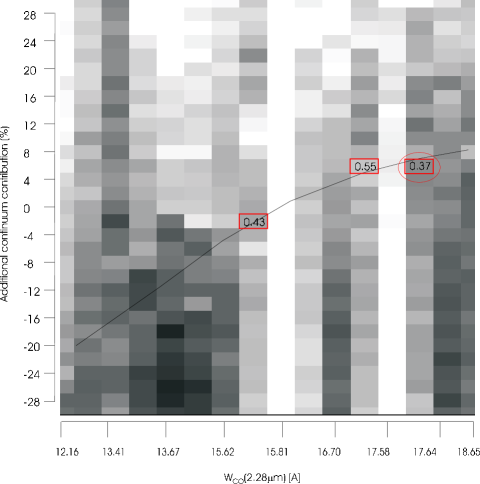
Figure 5: Visualization of the velocity dispersion determination for cluster W99-15.
Left: Greyscale shows the velocity dispersion (black $\approx$10 km s^-1 to white $\approx$27 km s^-1), contours show the corresponding $\chi^{2}$ (from 1.28 to 2.0). Arranged along the x-axis are different input supergiant template stars, arranged according to increasing CO equivalent width. The input spectra between labelled columns were created by averaging two neighbouring spectra. The y-axis arranges the template spectra by added or subtracted continuum contribution, ranging from -30% to +30%. The line was added to guide the eye along the regions of lowest $\chi^{2}$, which depends mainly on the CO equivalent width of the template spectrum matching that of the cluster. Some of the $\sigma$-values for the lowest $\chi^{2}$ in a column are labelled, and the three best fitting $\sigma$ values are boxed, with the corresponding $\chi^{2}$ value listed below the box. Right: The best fitting $\sigma$ value is chosen from the three $\sigma$ values with the lowest $\chi^{2}$ (they are marked with boxes in the left figure) by requiring that $\sigma$ depend only weakly on the selected wavelength range. The corresponding diagnostic map is shown, which displays the standard deviation in the velocity dispersion (grey scale, ranging between 0.05 (black) and 1.63 km s^-1 (white)). Out of the pre-selected three best fits, the third spectrum, located between the columns labelled “17.58” and “17.64” shows the lowest variations in velocity dispersion for the five wavelength regions. The numbers in the boxes give the standard deviation for the velocity dispersions for the three best cases. Thus, the best matching template (marked by an ellipse) has a W_CO of 17.6 Å and a continuum contribution of 6%, resulting in a velocity dispersion of 20.2 km s^-1, with a standard deviation of 0.37 km s^-1.

We applied the three criteria described in § 3.3.1 to our cluster data by creating a stellar template grid with CO(2.28$\mu$m) equivalent widths between 12.2Å and 18.7Å (we used the nine template stars listed in Table 2 and created intermediate spectra by averaging of two spectra), and added continuum levels of -30% to +30%. One of these maps is displayed in Figure 5. The greyscale image of velocity dispersions has a contour overlay of the corresponding $\chi^{2}$, and the minimum positions are to first order located at regions of comparable CO equivalent widths. We selected for the average $\sigma$ value only those template spectra which had a weak dependence of $\sigma$ on selected wavelength range, which is displayed on the second map in Figure 5, and additionally verified by visual inspection that the shape of the fit around the band-head is well-matched.

The best-fitting template for cluster [W99]15, for example, is a star with a CO equivalent width of 17.6Å, with an additional 6% continuum contribution. This matches very closely the predictions of stellar contributions from evolutionary synthesis models: For example, according to STARS (Sternberg (1998)), the K-band light in a cluster of 8.5 Myrs is composed of 95% M1/M2 type supergiants, $\approx 3$% hot main sequence stars and $\approx$1.5% A-G type supergiants.

The ISAAC and UVES observations gave an estimate of $\sigma$=14.0$\pm$0.8 and 14.3$\pm$0.5 km s^-1 for [W99]2, respectively, where the uncertainties in each measurement are the combination of the uncertainties in a single measurement as determined from the test data, and the deviations between different templates and fit wavelengths ranges. The difference in the estimated velocity dispersions is only 0.3 km s^-1. This difference is well within the random error we have estimated using the test data and demonstrates that there are unlikely to be any systematic differences in using the UVES and ISAAC data (or the I-band compared to K-band or the CaT plus weaker lines compared to the CO band-heads) to estimate the velocity dispersions.

We found that the best fitting models for the light profiles of the clusters were King models with tidal to core radii ratios of 15 (c=1.176) or 30 (c=1.477; both concentrations typically provided fits that were of indistinguishably good statistical significance but clearly better than the other fitted models, i.e., Gaussian or Moffat profiles). The effective radii of the observed clusters were approximately 4 pc, similar to what Whitmore et al. (1999) estimated as the average radius of the population of clusters in the Antennae. So while the selected clusters are among the most luminous in the Antennae, they are certainly not among the largest.

4.1 Estimating the Metallicities and Ages of the Clusters

Given the wide wavelength coverage of the UVES data, some interesting features are contained in the spectra. One such feature is the MgI line at 8806.8Å. This feature has been shown by Díaz et al. (1989) to be sensitive to the metallicity. The strength of this feature in two clusters is between 0.6 and 0.8Å, which according to the empirical calibration of the equivalent width of the MgI feature suggests approximately solar metallicity (there is significant scatter in the relationship between metallicity and line strength). However, the equivalent width of the MgI absorption feature in [W99]2 is $\approx$1.2Å, which indicates super-solar metallicity. Unfortunately, for the clusters with only ISAAC near-infrared spectroscopy, it is not possible to estimate the metallicities of the clusters from these data alone.

To determine the ages of the clusters, we followed the prescription outlined in Mengel et al. (2001), with the additional information from the CaT. This method relies on the equivalent widths of the CO-band head at 2.29$\mu$m, CaT lines, and the Br$\gamma$ emission line (where available for each cluster). The Br$\gamma$ emission strength estimates come from Mengel et al. (2001) or Mengel et al. (2001, in preparation) with the later estimates resulting from narrow band Br$\gamma$ imaging of the Antennae. We used the diagnostic plots from Leitherer et al. (1999) of the equivalent widths of these features versus age assuming an instantaneous burst, solar metallicity (but twice solar for cluster [W99]2), and a Salpeter IMF between 1 and 100 M_☉. The strength of using these features is that the equivalent width versus age relations have different dependencies as a function of age. Br$\gamma$ is strong in the early evolution of the cluster and weakens on the main sequence evolutionary time scale of the most massive stars with significant ionizing photon output (ages less than about 6-8 million years). The CaT lines reach significant equivalent widths at about 6 million years (as the I-band light becomes dominated by red supergiant stars) while the CO band-head at 2.29$\mu$m becomes significant at about 8 million years (as the K-band light becomes dominated by red supergiants). The combination of these diagnostics have a useful and relatively unambiguous age sensitivity to instantaneous burst populations over the age range from 0 to 20 million years, beyond which, the age determination ceases to be unambiguous.

From these line strengths we estimated the ages given in Table 3, ranging from about 6 to 10 million years, which reflects the selection criterion of strong CO absorption, required for the determination of the velocity dispersion (as discussed in § 2). Moreover, we note that the metallicity estimates can play a crucial role in determining the ages. As we discussed for [W99]2, we have evidence that it has a super-solar metallicity. In Mengel et al. (2001), we found that [W99]2 exhibits strong CO band-heads as well as relatively strong Br$\gamma$ emission and discussed the age determination of this cluster under the assumption of solar metallicity. Mengel et al. (2001) found that one age was difficult to reconcile with the measurements and speculated that the simultaneous Br$\gamma$ and strong CO band head could be reconciled with a single age if the low spatial resolution of our data allow for different physical regions of different ages to contribute to the final spectrum, the cluster had an extended duration of star-formation, or that shocks were present. Our finding that this cluster may have super-solar metallicity releaves this dilemma in that it is now possible to reconcile all of the measurements in that strong CO absorption now appears at an earlier age (at an age where Br$\gamma$ emission is also present). In this case, we now find the age of 6.6 Myrs instead of 8.1 Myrs under the assumption of solar metallicity. Further we note, in our current sample, [W99]2 is that only cluster that shows significant Br$\gamma$ emission and CO 2.29$\mu$m lines simultaneously.

5 Discussion and Implications

5.1 Are the Clusters Bound and Have They Undergone Mass Segregation?

The underlying assumption of any mass estimate using the velocity dispersion will be that the cluster is self-gravitating (i.e., bound). From the velocity dispersions and half-light radii we estimate that the crossing times ($t_{cross}\sim r_{hp}/\sigma$) range from about 1 to a few $\times$10⁵ yrs. We determined the ages of these clusters to be around 8 Myrs and thus these clusters have already survived for 20-50 crossing times. It is clear that at least initially, these clusters must have been gravitationally bound, and that the structure of these clusters is likely to be changing slowly over many crossing times. This assumption is also supported by N-body simulations performed by Portegies Zwart et al. (1999) on the evolution of a cluster with a similar concentration like the ones in our study. Core radius and density stay almost constant between 4 and 10 Myrs, the endpoint of their study. Only one IMF was used (Scalo), but we assume that these findings should be valid unless the IMF slope is very shallow (below $\alpha\approx 1.5$).

The stars are expected to be segregated by mass on the “two-body relaxation time-scale”. Given that we have an estimate of the velocity dispersion and mass densities, it is possible to estimate the two-body relaxation time-scale. Using the arguments in Spitzer & Hart (1971) we estimate that the half-light relaxation time scale is several 100 Myrs. Since the cluster ages are much less than this, dynamical mass segregation seems unlikely. However, several very young star clusters, like R136 in 30 Doradus (age around 4 Myrs, see e.g. Brandl et al., 1996) show evidence for mass segregation, which suggests that either the more massive stars formed preferentially near the center, or that the segregation occurs on a faster time-scale: N-body calculations by Portegies Zwart (2000) achieved some mass segregation within a few crossing times. If mass segregation was present in the Antennae star clusters, both the half mass radius and the velocity dispersion, and therefore the mass, would be underestimated by our calculations.

5.2 The Estimates of the Masses

Since we have argued that these clusters must have been gravitationally bound initially (although subsequent dynamical evolution and mass loss through massive star winds and supernova explosions may unbind the clusters), we can now use the Virial theorem, the light profiles (and under the assumption that the light distribution follows the mass distribution, i.e., the mass-to-light ratio is not a function of radius), and the velocity dispersion to estimate the masses of the clusters. The masses were derived assuming 1) that the best fitting profile was a King model (the light profiles were well fit with King models with concentrations of 1.176 or 1.477) 2) that the mass distribution follows the light profile, and 3) that the measured velocity dispersions were in fact not the central velocity dispersions but were projected velocity dispersion weighted by the projected light profile. Again, the corrections between the half-light radius and the core radius (defined in the King model) and central velocity dispersion and the measured velocity dispersion were given by those from the King models themselves (see, for example, McLaughlin 2000 for these relationships). The masses we derive are listed in Table 3 and range from about 6.5 $\times$10⁵ M_☉ to 4.7$\times$10⁶ M_☉. The uncertainties in the mass estimates given in Table 3 only represent the statistical uncertainties estimated for the velocity dispersion and half-light radius and do not represent any additional uncertainties due systematic errors (as might be caused by a radial dependence on the mass-to-light ratio, systematically over-estimating the size of the cluster, erroneous functional form of the light profile, etc).

Figure 6: The V-band light-to-mass ratios for the young compact clusters in the Antennae compared with models of Leitherer et al. (1999) for an instantaneous burst of total mass 10⁶ M_☉ with a power-law slope, solar metallicity , and a stellar mass range from 0.1 to 100 M_☉. The power-law slopes are 2.35 (solid line), 2.00 (dashed line), and 3.00 (dotted line). The points represent the data for the antennae clusters with V-band photometry from HST and with the extinction estimated as stated in the text. Unfortunately, cluster [WS95]355 is too faint to be detected in the HST WFPC-2 images. The error bars represent a combination of the error in the mass and the uncertainty in the photometry and extinction estimate was assumed to be 10%. The light-to-mass ratios shown take into account the mass lost through stellar winds and supernova over time.

We caution that while we believe the fits to the light profiles are robust, given that the HST data used to estimate the size scales has a resolution that is close to the measured half-light radii, it is possible that we have systematically over-estimated the cluster sizes. This could lead to a systematic over-estimate of the total dynamical masses by the same proportion. The relation between cluster concentration and mass is non-linear. For our typically best fitting models (c=1.176 or c=1.477), both lower or higher values would lead to a decrease in mass (by 2% if c=0.477 instead of 1.176, and by 25% if c=2 instead of 1.477). This means that unless the clusters are much more concentrated than estimated, the masses can be overestimated only slightly.

5.3 Mass-to-Light Ratios of the Clusters and Implications for the IMF

One of the critical parameters to understanding star-formation in and the dynamical evolution of these compact, young star-clusters is their initial mass function. If we find that these clusters are best described as having an IMF with significant numbers of low mass stars (say Salpeter slope down to 0.1 M_☉), then the dynamical evolution will be driven through the ejection of these numerous low mass stars by binaries and massive stars in the cluster. Moreover, the fraction of the total mass lost through stellar winds and supernova explosion will be relatively small (10s of percent; Leitherer et al. 1999). It is then likely, since the amount of overall ejected mass is relatively small compared to the total mass, for the clusters to remain bound and long-lived. If however, there is a lack or relative deficit of low mass stars (either through an IMF that is truncated at the low mass limit or that has a relatively flat slope), then the total mass loss from the cluster due to stellar ejection (since higher mass stars would then be more likely to get ejected) and the fraction of the total mass lost through stellar winds and supernova would also be proportionally higher both of which would tend to increase the likelihood that cluster becomes unbound (e.g., Chernoff & Weinberg 1990; Takahashi & Portegies Zwart 2000).

Figure 7: The K-band light-to-mass ratios for the young compact clusters in the Antennae compared with models of Leitherer et al. (1999) for an instantaneous burst of total mass 10⁶ M_☉ with a power-law slope, solar metallicity (we did not add the track for 2$\times$Z_☉, which would be appropriate for cluster [W99]2because the difference is below 0.1 dex, well within our uncertainties), and a mass range from 0.1 to 100 M_☉. The power-law slopes are 2.35 (solid line), 2.00 (dashed line), and 3.00 (dotted line). The points represent the data for the Antennae clusters with ground-based K-band photometry (Mengel et al. 2001, in preparation) and with the extinction estimated as stated in the text. The error bars represent a combination of the error in the mass and the uncertainty in the photometry and extinction estimate was assumed to be 10%. The model light-to-mass ratios shown take into account the mass lost through stellar winds and supernovae over time.

In the following we use the derived masses and ages, in combination with the photometry and extinction estimates, to constrain the IMFs of these clusters through the use of population synthesis models (see for example, Sternberg 1998). The approach uses a comparison of the cluster with population synthesis models to predict the mass-to-light ratios as a function of the cluster age. In our case, we can perform this comparison in both the V-band and the K-band, which is useful because these bands differ in their M/L-evolution with age and in their extinction sensitivities. For example, the K-band is less sensitive to the extinction than the V-band (by about a factor of 10) and also shows a strong dependence on age through the significant effect on the K-band luminosity when supergiants become prevalent in the cluster stellar population. There are also practical differences in the two bands. The K-band data are ground-based and hence are sensitive to our ability to remove the background from the photometry of the clusters and also might include contributions to their total magnitudes from other nearby clusters. The V-band data are HST WFPC-2 images and hence are less sensitive to contamination and background subtraction uncertainties. Although this last difference is partially mitigated by the fact that our K-band image used for this analysis has a seeing of $\approx$0$\aas@@fstack{\prime\prime}$4 to 0$\aas@@fstack{\prime\prime}$5.

Keeping these differences and limitations in mind, we attempt to constrain the functional form of the IMF in Figures 6 and 7. In the plot of the log L_K/M versus age, the most striking feature is that the clusters form two groups, several clusters have L_K/M at their estimated ages that seem best described with an IMF having a relatively flat slope, or perhaps slightly steeper slopes, but truncated low mass limits (higher than the 0.1 M_☉ in the model). For example, the difference in mass between a Salpeter IMF slope with an initial mass range from 0.1 – 100 M_☉ compared to a Salpeter IMF slope with an initial mass range from 1.0 – 100 M_☉ is a factor of 2.6. Such a difference would shift the Salpeter IMF slope line in Figures 6 and 7 upwards by 0.4 dex implying that a Salpeter IMF slope with an initial mass range from 1.0 – 100 M_☉ is consistent with the results for clusters [W99]1 and [W99]2. The results for clusters [W99]15 and [WS95]355 are more consistent with a steeper IMF slope, approximately 2.5 with an initial stellar mass range of 0.1 – 100 M_☉ or a steeper slope with a truncated lower mass. In the light-to-mass ratios in the V-band, this difference is less clear. The light-to-mass ratios for [W99]1 and [W99]15 give consistent results in both the K- and V-bands.

Similar results for young, compact clusters in nearby galaxies have also been presented. Sternberg (1998) using data from the literature for two clusters, one in NGC 1705 (NGC1705-1) and another in NGC 1569 (NGC1569-A), found that the light-to-mass ratio of these two clusters indicated rather shallow IMF slopes ($\approx$ 2.5 for NGC1569-A and $<$ 2 for NGC1705-1 if their IMFs extend down to 0.1 M_☉). Smith & Gallagher (2001) found in their analysis of M82-F that it either requires an extremely flat IMF slope ($\alpha$ $<<$ 2.0) or that it has a steeper IMF slope ($\alpha$ = 2.3) but then has a lower mass cut-off of about 2-3 M_☉. However, some caution is necessary in the interpretation of M82-F. The photometry of this cluster is rather uncertain given that it was heavily saturated in the HST images used by Smith & Gallagher (2001) to estimate its magnitude and the extinction (E_B-V =0.9$\pm$0.1). Smith & Gallagher (2001) also re-analysed some of the half-light radius and magnitude measurements of NGC1705-1 and NGC1569-A and although the detailed estimates of the light-to-mass ratios for NGC1705-1 differ, they come to the same conclusions as Sternberg (1998). We show a graphical comparison of our results with those obtained for M82-F, NGC1705-1, and NGC1569-A from Smith & Gallagher (2001) in Fig. 8.

Figure 8: The points are the same as in Fig. 6 but now with additional results from Smith & Gallagher (2001) for the clusters M82-F, NGC1705-1, and NGC1569-A. The results obtained for the clusters NGC1705-1 and NGC1569-A are similar to those in Sternberg (1998) except for NGC1705-1 which in Smith & Gallagher (2001) has a L_V/M lower by a factor of approximately two mainly due to their re-evaluation of the cluster half-light radius (revising the size upward by about a factor of 2).

If the segregation of the cluster points in Figure 7 is a real effect, it means that the IMF varies significantly between clusters. We do not yet have the possibility to disentangle lower mass cutoff and IMF slope, but the two different groups of clusters differ in their ratio of low- to high mass stars by approximately a factor 5 (“low” and “high” relating to stars below and above 3 M_⊙, respectively).

There has been substantial debate in the literature as to whether or not different environments lead to different forms of the IMF. While there does not exist a thorough understanding of the process of star-formation, possible mechanisms that have been investigated for determining the characteristics of the IMF are variations in the local thermal Jeans mass (e.g., Larson 1985; Klessen & Burkert 2001), turbulence (e.g., Elmegreen 1997), gravitationally-driven fragmentation (e.g., Larson 1985), cloud-cloud and star-star coalescence (e.g., Nakano 1966; Bonnell, Bate, & Zinnecker 1998) and several other processes (see for example, Larson (1999); Elmegreen (1999) and references therein). While it would be highly speculative to suggest that the range of IMF slopes and/or low mass cut-offs we observe supports or refutes any of these hypotheses for what physical processes are responsible for determining the characteristics of the IMF, it is useful to discuss what constraints these results might offer in understanding the origin of the IMF.

There are two attractive hypotheses for explaining the observed segregation. One is that perhaps the difference in the relative number of low mass stars is related to the environment in which the cluster is born. Clusters [W99]15 and [WS95]355 suffer greater extinction on average than most clusters in the Antennae and both lie in the over-lap region of the two merging disks. Clusters [W99]1 and [W99]2 lie in the “western loop” of the Antennae’s northern most galaxy, NGC4038 and have relatively low extinctions (A_V$\approx$0.3 magnitudes). In spite of the clusters having similar ages, the environments of [W99]15 and [WS95]355 appear to be much more rich in dust and gas (Whitmore & Schweizer 1995; Wilson et al. 2000; Mengel et al. 2001). However, cluster [W99]16, while physically lying near the clusters [W99]15 and [WS95]355, appears to suffer much less extinction. Presumably, since the region where [W99]15, [W99]16, and [WS95]355 were formed is also the region where the two disks are interacting, the gas pressure (both the thermal and turbulent) would be high due to dynamical interactions of the two interstellar media. The local thermal Jeans mass, which is considered to play a role in setting the mass scale for low mass stars (e.g., Larson 1999), is proportional to T²P^-1/2, where T and P are the total pressure and temperature (e.g., Spitzer 1978). Clouds with low temperature and/or high pressures would form clusters with IMFs weighted towards low mass stars, which would be applicable for the more extinguished clusters. Conversely, clouds that are collapsing in relatively low extinction, gas poor, more quiescent regions might be influenced by the ionizing radiation of nearby young clusters raising its gas temperature. Such a situation would favor the formation of clusters with IMFs that have relatively large fractions of high mass stars. Such an idea might also explain the mass functions of NGC1569-A and NGC1705-1 whose relatively low metallicities could favor high gas temperatures (by reduced cooling and high background radiation fields). Thus studies of young compact clusters in the Antennae and other galaxies appear to agree with the expectation from the low mass scaling set by the Jeans mass.

The second plausible hypothesis is that in Fig. 7 and 8 the clusters with relatively large ratios of light-to-mass are also among the lower mass clusters. N1569-A, N1705-1, M82-F, [W99]1, and [W99]2 all have masses less than about 2 $\times$ 10⁶ M_☉. Clusters [W99]15, [W99]16, [WS95]355 all have masses greater than 3 $\times$ 10⁶ M_☉. While the total mass of a cluster influencing the observed IMF has been discussed in the literature, it is most commonly discussed within the context of random sampling of stars in clusters with relatively few stars (e.g., Elmegreen 1999). The Antennae clusters are certainly not in this limit since they have many $\times$ 10⁵ stars. However, it may be that there is a process internal to the cluster that inhibits preferentially the formation of low mass stars and that this may scale roughly with the mass of the cluster. One possibility is that the massive stars through radiation pressure might inhibit or shut off the formation of low mass stars.

Obviously using compact, young star clusters in the Antennae and other galaxies to provide observational constraints on the processes that lead to the characteristics of the IMF will require much more observational and theoretical work. However, even the relatively sparse and modest results provided here and in the literature are tantalizing and show the promise of this type of observation in advancing our understanding of the process of cluster and star-formation.

5.4 The Evolution of the Most Massive Clusters: Will They Dissolve?

Are these young clusters progenitors of the old globular cluster systems that we observe in normal galaxies? If they are, how would the population of young clusters need to evolve to have a mass distribution that resembles that of the old globular cluster system? These fundamental questions can only be addressed when we have characterized the masses, initial mass functions, and strength and change in the gravitational potential in which these clusters form and evolve.

Various models have been constructed to follow the evolution of clusters with structure similar to globular clusters (see Spitzer (1987) and references therein). Perhaps the most relevant for this study are those that employ the Fokker-Planck approximation in solving the dynamics of the constituent cluster stars (Cohn (1979); Chernoff & Weinberg (1990); Takahashi & Portegies Zwart (2000)). The dynamics of Fokker-Planck models are relatively simple to calculate compared to full N-body models and thus other astrophysical effects that might be important to the dynamical evolution of the cluster can be included (such as including a range of stellar masses distributed with a realistic IMF, stellar mass loss, stellar evolution, etc). While these models have their limitations, the results of these studies provides a useful guide on how these young, compact clusters of the Antennae might evolve given our determined constraints on the shape of their IMFs and concentrations. The Fokker-Planck models (e.g., Cohn (1979); Chernoff & Weinberg (1990); Takahashi & Portegies Zwart (2000)) suggest the most likely survivors are those clusters that are either more highly concentrated (King model concentrations of greater than 1.0-1.5), and/or those with steep IMFs. This is shown graphically in Fig. 9 where we have reproduced approximately a figure from Takahashi & Portegies Zwart (2000) (their Figure 8) that shows which range of cluster parameters the clusters are long-lived or disrupt. For the range of plausible IMF slopes that we have determined (assuming, as in the models, that the IMF extends down to sub-solar masses), the models suggest that clusters that are about as concentrated as we have observed in the Antennae will survive for at least a few Gyrs. Even though we have no independent constraint on the lower mass limit of the stellar mass function, it is interesting that models with steep IMF slopes are also robust against disruption. From these models alone it is difficult to tell if the clusters are able to withstand the disruptive tendencies of the large mass loss they suffer if the lower mass limit (0.1 M_☉ in Figs. 6 and 7) is raised and the IMF slope steepened, such that the observed light-to-mass ratio constraints are met. The limited number of models so far generated seems to indicate that clusters with very steep slopes ($\alpha$ $>$ 3) of their IMF are robust. More modeling is obviously needed to answer this question quantitatively and definitively.

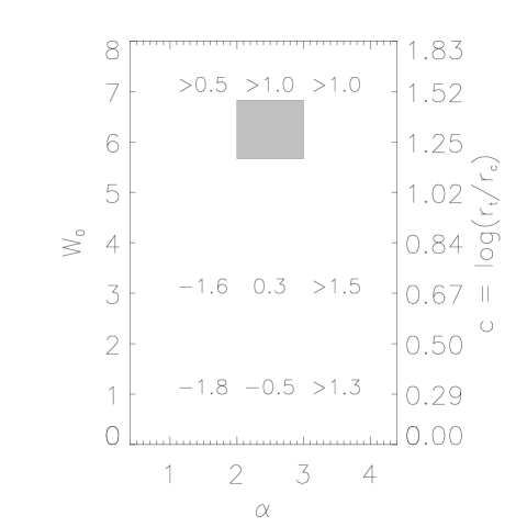
Figure 9: This is a modified reproduction of a figure from Takahashi & Portegies Zwart (2000; their Figure 8) showing the ages at the endpoint of evolution for modeled clusters. The clusters were characterized by scaled central potentials, W₀ (which is related to the concentration, c, as shown in the ordinate on the right side) and IMF slopes ($\alpha$). The numbers in the grid give the ages at the endpoint of the evolution (disruption or core collapse) as log(age [Grys]). Clusters with values below 0.3 (corresponding to 2 Gyrs) were disrupted by dynamical processes over time, the others experienced core collapse. The grey box shows the region where the clusters in the Antennae are observed to lie. This suggests that the clusters are relatively long lived.

Even if the clusters survive, it is obviously important to have some indication of how much mass loss they may undergo as they age. For some of the cluster parameters, these models suggest that these clusters may lose significant amounts of mass ($>$50%, sometimes much greater; Takahashi & Portegies Zwart (2000)). Clusters with steep IMF slopes ($\alpha$ $>$ 2.5) which are compact (c$>$1.5) apparently suffer large mass loss (may lose more than 90% of their total initial mass; Takahashi & Portegies Zwart (2000) but also Chernoff & Weinberg (1990) whose models suggest that perhaps some of these high mass loss clusters are disrupted). Therefore, it is easily possible for these cluster to survive, but over their lifetimes, they will have much lower masses than when they are as young as the clusters we have observed here. It is through such strong mass loss that the young compact clusters in the Antennae may evolve into something similar to the population of clusters observed in galaxies generally (e.g., Fritze-v. Alvensleben 1998; 1999).

There are limitations in the models that might in fact lead to higher mass loss rates and possibly easier disruption of clusters for a given set of initial conditions than predicted in the models. One is that the tidal field is much more complex and stronger than what is assumed in the models which is static or a simple orbital potential in a disk. In a strong and variable tidal field, the mass loss rates would undoubtedly go up (e.g., Gnedin & Ostriker 1997). However, very little is known about the tidal field over time on the scales of the clusters and such an analysis would require a greater understanding of the mass distribution in galaxies than we currently have. Therefore, literal interpretations of the evolution of clusters as indicated by the models should be viewed with some caution.

In summary, given what we have learned in this analysis, it is likely that the most massive clusters are able to survive in the galaxian environment in which they are born, and do not abruptly disappear. Since we cannot constrain the lower mass limit of the stellar mass function it is possible that the clusters are easier to disrupt than we have suggested here. The amount of mass-loss they will undergo is uncertain but is likely to be a large percentage of their initial masses thereby providing a mechanism were the massive clusters studied here can evolve to look more like a typical cluster in a galaxy like the Milky Way.

6 Summary and Conclusions

In order to estimate the masses of young compact clusters in the interacting pair of galaxies NGC 4038/4039 (“the Antennae”), we have measured the velocity dispersions of 6 clusters using high resolution optical and near-IR spectroscopy conducted at the ESO-VLT. The velocity dispersions were estimated using the stellar absorption features of CO at 2.29 $\mu$m and metal absorption lines at around 8500Å including lines of the Calcium Triplet. To estimate the masses, we measured the size scales and light profiles from archival HST WFPC-2 (see Whitmore et al. 1999). The ages of individual clusters were estimated using the equivalent widths of the CO band-head at 2.29 $\mu$m, the CaT, and the Br$\gamma$ emission line (estimated from data in Mengel et al. 2001 and Mengel et al. 2001, in preparation). Our principle results from this analysis are:

• The clusters have ages of about 8 Myrs. This is a selection effect since we selected the clusters based on other observations indicating that they had ages of about 10 Myrs to ensure they had strong CO$\lambda$2.29 $\mu$m and CaT absorption lines for determining the velocity dispersions.

• The best fitting light profiles are consistent with King models of concentration parameters, c, of either 1.176 or 1.477 (tidal to core radius ratios of 15 or 30 respectively). The half-light radii from these fits are all around 4 pc which is typical of the young compact clusters in the Antennae (Whitmore et al. 1999).

• The measured velocity dispersions were all between 9 and 21 km s^-1. Combining the velocity dispersions, half-light radii, and parameters of a King model under the assumption that the clusters are in approximate Virial equilibrium (an assumption which is supported by our estimate that the clusters have already survived for 10s of crossing times) yields mass estimates that range from 6.5 $\times 10^{5}$ to 4.7 $\times 10^{6}$M_☉. These masses are large compared to typical masses of a globular cluster ($\sim 1\times 10^{5}$M_☉), but this not surprising, since we selected the brightest clusters for our first analysis.

• Comparing the cluster light-to-mass ratios with stellar synthesis models (Leitherer et al. 1999) suggests that these clusters may exhibit a range of initial mass functions, with clusters in the “over-lap” region showing evidence for a steeper IMF slope than those clusters in less extinguished regions. However, with only five clusters observed this result needs to be substantiated with observations of more clusters.

• Results of Fokker-Planck simulations of compact clusters with concentrations and IMF parameters similar to those found for the young, compact clusters in the Antennae studied here, suggest that these clusters are likely to be long-lived (more than a few Gyrs) and may lose a substantial fraction of their total mass.