DSF-37-2001, MPI-PhT/2001-51, astro-ph/0111408
 
A precision calculation of the effective number of cosmological neutrinos

Abstract

The neutrino energy density of the Universe can be conveniently parametrized in terms of the so-called effective number of neutrinos, $N_{\nu}^{\rm eff}$. This parameter enters in several cosmological observables. In particular it is an important input in those numerical codes, like CMBFAST, which are used to study the Cosmic Microwave Background anisotropy spectrum. By studying the neutrino decoupling with Boltzmann equations, one can show that this quantity differs from the number of massless neutrino species for an additional contribution due to a partial heating of neutrinos during the $e^{\pm}$ annihilations, leading to non thermal features in their final distributions. In this paper we review the different results obtained in the literature and perform a new analysis which takes into account, in a fully consistent way, the QED corrections at finite temperature to the photon and $e^{{\pm}}$ plasma equation of state. The value found for three massless active neutrinos is $N_{\nu}^{\rm eff}=3.0395$, in perfect agreement with the recommended value used in CMBFAST, $N_{\nu}^{\rm eff}=3.04$. We also discuss the case of additional relativistic relics and massive active neutrinos.

, , ,

1 Introduction

At temperatures below the muon mass and above $\sim 10$ MeV, the Universe is filled by a plasma of photons, electrons, positrons, and neutrinos, kept in thermodynamical equilibrium by the electroweak interactions. As the temperature drops below this value, the rate of weak interactions starts to be comparable with the Universe expansion rate, and neutrinos decouple from the electromagnetic $\gamma,\,e^{\pm}$ plasma. For most practical purposes, it is accurate enough to consider the freeze-out of neutrinos as fully achieved at temperatures of about $2-3$ MeV. In this limit neutrinos do not share any entropy release from $e^{\pm}$ annihilations, once the temperature drops further, below the electron mass. Assuming that all the entropy produced by the annihilations is transferred to photons, their temperature $T$ is increased with respect to the neutrino temperature by the well known factor $T/T_{\nu}=\left(11/4\right)^{1/3}$ (see, for example, [1]). Actually more accurate calculations show that neutrinos are still slightly interacting with the electromagnetic plasma and thus receive a small portion of the entropy from $e^{\pm}$ annihilations [2]. Neutrinos with higher momenta are more heated, since, in the relevant range of energies, weak interactions get stronger with rising energy. This produces a momentum dependent distortion in the neutrino spectra from the equilibrium Fermi–Dirac behaviour.

A further, though smaller, effect on $T/T_{\nu}$ is induced by finite temperature QED corrections to the electromagnetic plasma. In fact electromagnetic interactions modify the $e^{\pm}$ and $\gamma$ dispersion relations, and thus the energy density and pressure of the plasma. More precisely, the energy density is lowered so that the $e^{\pm}$ annihilation phase releases less entropy with respect to the non-interacting particle limit calculation. Since most of this energy ends up into photons, this decrease results in a smaller $T/T_{\nu}$ ratio [3].

While any direct observation of the actual distortions in the neutrino distributions is out of question, nevertheless we can hope that the increase of the total energy of the relic neutrinos may have a sizeable effect on the expansion rate of the Universe. The energy density stored in relativistic species, $\rho_{R}$, is customarily given in terms of the so-called effective number of neutrino species [4, 5], $N_{\nu}^{\rm eff}$, through the relation

$$\rho_{\rm R}=\left[1+\frac{7}{8}\left(\frac{4}{11}\right)^{4/3}\,N_{\nu}^{\rm eff}\right]\,\rho_{\gamma}\,\,,$$ (1)

where $\rho_{\gamma}$ is the energy density of photons, whose value today is known from the measurement of the Cosmic Microwave Background (CMB) temperature. Eq. (1) can be also written as

$$N_{\nu}^{\rm eff}\equiv\left(\frac{\rho_{R}-\rho_{\gamma}}{\rho^{0}_{\nu}}\right)\left(\frac{\rho^{0}_{\gamma}}{\rho_{\gamma}}\right)\,,$$ (2)

where $\rho_{\nu}^{0}$ denotes the energy density of a single specie of massless neutrino with an equilibrium Fermi-Dirac distribution, and $\rho^{0}_{\gamma}$ is the photon energy density in the instantaneous neutrino decoupling approximation. The normalization of $N_{\nu}^{\rm eff}$ is such that it gives $N_{\nu}^{\rm eff}=3$ in the standard case of three families of massless neutrinos, in the limit of an instantaneous decoupling. In principle, $N_{\nu}^{\rm eff}$ can receive contribution from other relativistic relics with energy density $\rho_{X}$ as well. In the following we will mostly restrict our analysis to the standard case, but we will further consider this more general framework in Section 4.

As we will discuss below, when considered separately, the non instantaneous neutrino decoupling gives $\Delta N_{\nu}^{\rm eff}\equiv N_{\nu}^{\rm eff}-3\simeq 0.034\,$ [6, 7, 8], while QED effects contribute for about $\Delta N_{\nu}^{\rm eff}\simeq 0.011\,$ [3]. Could the two effects be added linearly, they therefore would produce a final value $N_{\nu}^{\rm eff}\simeq 3.045$. Recently, these effects have been reconsidered in [9]. This work combines the results for the non instantaneous neutrino decoupling obtained by a numerical calculation in [10] and then replacing the ratio $T/T_{\nu}=\left(11/4\right)^{1/3}$ with the value obtained by considering QED corrections. This procedure may provide a good estimate, but it is worth pointing out that, since QED effects modify several points of the Boltzmann equations describing neutrino decoupling, it is advisable to study any possible interplay of the two effects. Actually a precision calculation of this kind, where both these effects are included at the same time, is still lacking, and it is the aim of the present paper. We will show that this interplay ends up in a $10\%$ smaller total correction to $N_{\nu}^{\rm eff}$ than what would be obtained by simply adding the two contributions. We also notice that the calculation of [10] seems to underestimate the corrections from non instantaneous neutrino decoupling with respect to the result found in [6, 7, 8]. Our analysis is based on a numerical code described in [8], which has been modified to take into account QED finite temperature effects.

From the observational point of view the effects considered in this paper are too small to influence Big Bang Nucleosynthesis (BBN), since they produce a change in the ⁴He mass fraction, $\Delta Y(^{4}\mbox{He})\sim 10^{-4}$  [8, 11, 12], which is smaller than the actual theoretical, $5~{}10^{-4}$ [12, 13], and experimental, $\;\raise 1.29167pt\hbox{$>$\kern-7.5pt\raise-4.73611pt\hbox{$\sim$}}\;2~{}10^{-3}$ [14], uncertainties on this quantity. This change is actually slightly larger when one takes into account the effect of flavour neutrino oscillations, as recently shown in [15]. More promisingly, they might be detected via future precision CMB anisotropy measurements at high multipoles, since cosmic variance prevents their resolution on scales probed by present balloon experiments. According to a recent analysis [16] (see also [13, 17, 18, 19, 20, 21]), CMB temperature measurements by the Planck satellite experiment will be able to provide a measure of the relativistic energy density with a precision of about $\Delta N_{\nu}^{\rm eff}\simeq 0.2\,$, without any strong prior on the other cosmic parameters. Furthermore, as discussed in [22], the situation is more promising if polarization measurements will be available, and some stronger priors are imposed on other cosmological parameters, enforced for example by independent measurements. In this case, $\Delta N_{\nu}^{\rm eff}$ would be determined with an accuracy comparable or, according to [22], even higher than the order of magnitude of the effects we are here considering. We notice that in the CMB data analysis the presence of a non vanishing $\Delta N_{\nu}^{\rm eff}$ is already considered with, for example, a recommended default value for three massless active neutrinos $N_{\nu}^{\rm eff}=3.04$ in the CMBFAST code [23] . A precise check of this important parameter is therefore mandatory.

The paper is organized as follows. In Section 2 we summarize the set of equations and our numerical approach to compute the neutrino distortion due to their incomplete decoupling during the $e^{\pm}$ annihilation phase. In Section 3 we also consider the corrections to the equation of state of $e^{{\pm}}$ and $\gamma$ plasma due to QED effects at finite temperature, showing how these effects modify the numerical computation of Section 2, and we present our results. We also discuss the general case of extra relativistic degrees of freedom and of massive active neutrinos in Section 4. Finally our conclusions are reported in Section 5.

2 Corrections from to the non instantaneous decoupling

The effects of non-instantaneous neutrino decoupling have been addressed in several studies, either based on analytical methods [2], on numerical analysis with some simplifying approximations [24, 25, 26, 27], or finally on full numerical computations, which solve the Boltzmann equations until neutrinos are completely decoupled [6, 7, 8, 10, 28].

The procedure is easily summarized. Following the notation of [6, 8], a convenient choice for the time variable is given by $x\equiv m\,R$, where $R(t)$ is the scale factor of the Universe (chosen to have dimension of length) and $m$ some reference mass, taken to be the electron mass as in [8]. We also introduce the dimensionless comoving momentum $y\equiv p\,R\,$, and the rescaled photon temperature $z\equiv T\,R\,$. In this notation, the Boltzmann equations for the neutrino distributions can be written in the form

$$\frac{d}{dx}\,f_{\nu_{\alpha}}\left(x,y\right)=\frac{1}{x\,H}\,I_{\nu_{\alpha}}\,\left[f_{\nu_{e}},f_{\nu_{x}}\right]\,\,,$$ (3)

where $H$ is the Hubble parameter, while $I_{\nu_{\alpha}}$ represents the collisional integral, in momentum space $y$, for the single neutrino specie $\nu_{\alpha}$, and is a functional of all neutrinos and electron/positron distributions. For the processes of interest (see [6] for the detailed calculation), some of the integrations appearing in the $I_{\nu_{\alpha}}$ can be analytically performed, and the collisional integrals can be reduced to two-dimensional integrals. In the range of temperatures we are interested in, electron neutrinos experience charged current interactions due to the presence of $e^{\pm}$ in the thermal bath, while all active neutrino flavours interact via neutral current interactions. For this reason, the nonequilibrium corrections to the distribution function $f_{\nu_{e}}$ are different from those of the other two neutrino species $f_{\nu_{x}}$ ($x$ denoting both $\mu$ and $\tau$).

The two Boltzmann equations for $f_{\nu_{e}}$ and $f_{\nu_{x}}$ must be supplemented by the continuity equation

$$\frac{d}{dx}{\bar{\rho}}\left(x\right)=\frac{1}{x}\left({\bar{\rho}}-3\,{\bar{P}}\right)\,\,,$$ (4)

where ${\bar{\rho}}=\rho\left(x/m_{e}\right)^{4}\,$, ${\bar{P}}=P\left(x/m_{e}\right)^{4}\,$, and $\rho$ and $P$ are the energy density and pressure of the $\gamma,\,e^{\pm},\,\nu$ plasma. Eq. (4) can be rewritten as an evolution equation for the quantity $z\,$ which gives the ratio $T/T_{\nu}$. In case of instantaneous neutrino decoupling, the asymptotic value of $z$, denoted by $z^{0}\,$, results to be the well-known value $(11/4)^{1/3}$.

As in Ref. [8] the unknown neutrino distributions are parametrized as

$$f_{\nu_{\alpha}}\left(x,y\right)=\frac{1}{{\rm e}^{y}+1}\,\left[1+\sum_{i=0}^{\infty}\,a_{i}^{\alpha}(x)\,P_{i}\left(y\right)\right]\,,$$ (5)

where $P_{i}(y)$ are orthonormal polynomials with respect to the Fermi function weight

$$\int_{0}^{\infty}\frac{dy}{{\rm e}^{y}+1}\,P_{i}\left(y\right)\,P_{j}\left(y\right)=\delta_{ij}\,\,.$$ (6)

By substituting Eq. (5) into Eqs. (3), one gets

$$\frac{d}{dx}\,a_{i}^{\alpha}(x)=\frac{1}{xH}\,\int_{0}^{\infty}dy_{1}\,P_{i}\left(y_{1}\right)\,I_{\nu_{\alpha}}\left[f_{\nu_{e}},f_{\nu_{x}}\right]\,\,.$$ (7)

Since at high temperature the neutrinos are in thermal equilibrium, the initial condition for the coefficients is $a_{i}^{\alpha}=0$.

To perform the numerical computation it is necessary to truncate the infinite series in Eq. (5) at some finite value $n$, where the choice of $n$ depends on the accuracy we do require on the results; it is found in [8] that $n=3$ gives an accuracy of about $1\%$ in the neutrino distortions. In this case, the asymptotic value found for $z$, denoted by $z^{\rm fin}$, slightly differs from the instantaneous decoupling result $z^{0}$

$$\frac{\delta z}{z^{0}}\equiv\frac{z^{\rm fin}-z^{0}}{z^{0}}=-1.406{\cdot}10^{-3}\,\,.$$ (8)

The final neutrino distribution functions show a non thermal behaviour due to the presence of non vanishing ripple terms. Having fixed $n=3$, we rewrite the expression of Eq. (5) in the form

$$f_{\nu_{\alpha}}^{\rm fin}\left(y\right)=\frac{1}{{\rm e}^{y}+1}\,\left(1+10^{-4}\sum_{i=0}^{3}c^{\alpha}_{i}~{}y^{i}\right)\,\,,$$ (9)

and report the final values for the coefficients $c^{\alpha}_{i}$ in Table 1. By using Eq. (9) it is now immediate to compute the additional contribution to the neutrino energy density due to incomplete decoupling. Defining

Flavour ($\alpha$)	$c^{\alpha}_{0}$	$c^{\alpha}_{1}$	$c^{\alpha}_{2}$	$c^{\alpha}_{3}$
$e$	-2.556	-2.739	6.133	-0.1477
$\mu,\tau$	-2.049	-2.259	3.145	-0.1129

Table 1: Values of the coefficients of Eq. (9) from [8] (QED effects not included).

$$\frac{\delta\rho_{\nu_{\alpha}}}{\rho_{\nu}^{0}} \equiv \frac{\int_{0}^{\infty}dy~{}y^{3}~{}f_{\nu_{\alpha}}^{\rm fin}(y)}{\int_{0}^{\infty}dy~{}y^{3}~{}\left({\rm e}^{y}+1\right)^{-1}}-1$$

$$= 10^{-4}\left(c^{\alpha}_{0}+2700\left(\frac{\zeta(5)}{7\pi^{4}}\right)c^{\alpha}_{1}+310\left(\frac{\pi^{2}}{147}\right)c^{\alpha}_{2}+12150\left(\frac{\zeta(7)}{\pi^{4}}\right)c^{\alpha}_{3}\right)\,\,,$$

one obtains, for the values of Table 1, $\delta\rho_{\nu_{e}}/\rho_{\nu}^{0}=0.953\%$ and $\delta\rho_{\nu_{x}}/\rho_{\nu}^{0}=0.399\%$. Finally, from the definition of $N_{\nu}^{\rm eff}$ of Eq. (1), it is straightforward to get the following expression

$$N_{\nu}^{\rm eff}=\left(\frac{z^{0}}{z^{\rm fin}}\right)^{4}\left(3+\frac{\delta\rho_{\nu_{e}}}{\rho_{\nu}^{0}}+2\frac{\delta\rho_{\nu_{x}}}{\rho_{\nu}^{0}}\right)\simeq\left(3-12\frac{\delta z}{z^{0}}+\frac{\delta\rho_{\nu_{e}}}{\rho_{\nu}^{0}}+2\frac{\delta\rho_{\nu_{x}}}{\rho_{\nu}^{0}}\right)\,\,,$$ (11)

which gives the effective number for three massless active neutrinos for temperatures below the neutrino decoupling ($\sim 1$ MeV). The values found from the numerical analysis then give $N_{\nu}^{\rm eff}=3.0345$, which fixes the additional contribution to be $\Delta N_{\nu}^{\rm eff}=0.0345$. Notice that from Eq. (11), $\Delta N_{\nu}^{\rm eff}$ takes two contributions. The term proportional to $\delta z/z^{0}$ accounts for the smaller profit that photon temperature gets from $e^{\pm}$ annihilations, whereas the contributions due to $\delta\rho_{\nu_{e,x}}/\rho^{0}_{\nu}$ are a measure of the non thermal behaviour of neutrino distribution functions. These two terms are indeed of the same size.

Remarkably, our results are in very good agreement with a previous analysis performed applying a different numerical technique [6, 7]. They find $\delta z/z^{0}=(-1.37{\pm}0.02){\cdot}10^{-3}$, and an increase of energy with respect to the instantaneous decoupling case of $\delta\rho_{\nu_{e}}/\rho_{\nu}^{0}=\left(0.946{\pm}0.001\right)\%$ for the electron neutrinos and of $\delta\rho_{\nu_{x}}/\rho_{\nu}^{0}=\left(0.398{\pm}0.001\right)\%$ for the other two species. These values give the effective number of neutrino species $N_{\nu}^{\rm eff}=3.0340{\pm}0.0003\,$.

On the other hand we disagree with the results of [10], where by solving the same Boltzmann equations it is found $\delta\rho_{\nu_{e}}/\rho_{\nu}^{0}=0.607\%$, $\delta\rho_{\nu_{x}}/\rho_{\nu}^{0}=0.256\%$ and $\delta z/z^{0}=-0.888{\cdot}10^{-3}\,$, which finally gives $N_{\nu}^{\rm eff}=3.022$. In both calculations [6, 7] and [10], the integral–differential Boltzmann equations are solved through a grid in momentum space. The grid adopted in [10] extends to a larger momentum range than the one of [6, 7]. The grid used in [6, 7] is however denser in the interval $0.1<y\,\left(m/{\rm MeV}\right)<20\,$. For neutrino distributions in thermal equilibrium, the $97.5\%$ of the energy density comes from particles with momentum in the range $1<y\,\left(m/{\rm MeV}\right)<10\,$. According to the analysis of [7], the different results of [10] may be due to a lack of precision in this most relevant interval. To conclude, we can only point out that the beautiful agreement of our findings with what obtained in [6, 7], despite of the rather different numerical method, make us rather confident on our result for $N_{\nu}^{\rm eff}$.

3 Corrections from QED at finite temperature

Finite temperature QED corrections modify in several points the calculations of neutrino decoupling described till now. First, through the change on the electromagnetic plasma equation of state, they affect Eq. (4). Moreover, since $e^{\pm}$ masses are renormalized by a finite temperature term, the r.h.s. of Eq.s (3) and (7) should be modified correspondingly. Finally, the change of energy density modifies the expansion rate $H$ in the Boltzmann equations (3). The effects of these corrections on neutrino decoupling temperature have been considered in [29]. Their analysis is however in the framework of the instantaneous neutrino decoupling limit, therefore they do not consider the non thermal effects described in the previous Section.

The change in the electromagnetic plasma equation of state can be evaluated by first considering the corrections induced on the $e^{\pm}$ and photon masses. They can be obtained perturbatively by computing the loop corrections to the self-energy of these particles. For the electron/positron mass, up to order $\alpha\equiv e^{2}/\left(4\,\pi\right)$ we find the additional finite temperature contribution [3] 

$$\delta m_{e}^{2}\!\!\! \!\!\!\left(p,\,T\right)=\frac{2\,\pi\,\alpha\,T^{2}}{3}+\frac{4\,\alpha}{\pi}\,\int_{0}^{\infty}dk\,\frac{k^{2}}{E_{k}}\,\frac{1}{{\rm e}^{E_{k}/T}+1}$$ (12)

$$- \frac{2\,m_{e}^{2}\,\alpha}{\pi\,p}\,\int_{0}^{\infty}dk\,\frac{k}{E_{k}}\,\log\left|\frac{p+k}{p-k}\right|\frac{1}{{\rm e}^{E_{k}/T}+1}\,\,,$$

where $E_{k}\equiv\sqrt{k^{2}+m_{e}^{2}}$. While the first two terms of this expression depend on the plasma temperature $T$ only, the last one depends on the $e^{\pm}$ momentum $p\,$ as well. However, by averaging this term over the equilibrium $e^{\pm}$ distribution, one easily finds that it contributes for less than $10\,\%$ to $\delta m_{e}^{2}\,$. For this reason we will neglect it in the following (see also [12]).

The renormalized photon mass in the electromagnetic plasma is instead given, up to order $\alpha$, by [29]

$$\delta m_{\gamma}^{2}\left(T\right)=\frac{8\,\alpha}{\pi}\,\int_{0}^{\infty}dk\,\frac{k^{2}}{E_{k}}\,\frac{1}{{\rm e}^{E_{k}/T}+1}\,\,.$$ (13)

The corrections (12) and (13) modify the corresponding dispersion relations as $E_{i}^{2}=k^{2}+m_{i}^{2}+\delta m_{i}^{2}\left(T\right)\,$ ($i=e,\,\gamma$). This in turn affects the total pressure and the energy density of the electromagnetic plasma

$$P = \frac{T}{\pi^{2}}\,\int_{0}^{\infty}dk\,k^{2}\,\,\log\left[\frac{\left(1+{\rm e}^{-E_{e}/T}\right)^{2}}{\left(1-{\rm e}^{-E_{\gamma}/T}\right)}\right]\,\,,$$ (14)

$$\rho = -P+T\,\frac{dP}{dT}\,\,.$$ (15)

Expanding $P$ with respect to $\delta m_{e}^{2}$ and $\delta m_{\gamma}^{2}$, one obtains the first order correction

$$P^{\rm int} = -\int_{0}^{\infty}\frac{dk}{2\,\pi^{2}}\left[\frac{k^{2}}{E_{k}}\,\frac{\delta m_{e}^{2}\left(T\right)}{{\rm e}^{E_{k}/T}+1}+\frac{k}{2}\,\frac{\delta m_{\gamma}^{2}\left(T\right)}{{\rm e}^{k/T}-1}\right]\,\,.$$ (16)

Note that an important factor $1/2$ must be introduced for not double counting the renormalization effect on the total pressure, which now reads $P=P^{0}+P^{\rm int}$ [3], $P^{0}$ being the value of the pressure for the non-interacting particle gas. The energy density is then obtained by using $P$ in Eq. (15).

Flavour ($\alpha$)	$c^{\alpha}_{0}$	$c^{\alpha}_{1}$	$c^{\alpha}_{2}$	$c^{\alpha}_{3}$
$e$	-2.507	-2.731	6.010	-0.1419
$\mu,\tau$	-2.003	-2.196	3.061	-0.1091

Table 2: Values of the coefficients of Eq. (9) when QED effects are included.

The presence of the additional contributions $P^{\rm int}$ and $\rho^{\rm int}$ modify the evolution equation for $z$ contained in Eq. (4), which now reads

$$\frac{dz}{dx}=\frac{\frac{x}{z}J(x/z)-\frac{1}{2\pi^{2}z^{3}}\int_{0}^{\infty}~{}dyy^{3}\left(\frac{df_{\nu_{e}}}{dx}+2\frac{df_{\nu_{x}}}{dx}\right)+G_{1}(x/z)}{\frac{x^{2}}{z^{2}}J(x/z)+Y(x/z)+\frac{2\pi^{2}}{15}+G_{2}(x/z)}\,,$$ (17)

where

$$G_{1}(\omega) = 2\pi\alpha\left[\frac{1}{\omega}\left(\frac{K(\omega)}{3}+2K(\omega)^{2}-\frac{J(\omega)}{6}-K(\omega)~{}J(\omega)\right)\right.$$

$$+ \left.\left(\frac{K^{\prime}(\omega)}{6}-K(\omega)~{}K^{\prime}(\omega)+\frac{J^{\prime}(\omega)}{6}+J^{\prime}(\omega)~{}K(\omega)+J(\omega)~{}K^{\prime}(\omega)\right)\right]$$

$$G_{2}(\omega) = -8\pi\alpha\left(\frac{K(\omega)}{6}+\frac{J(\omega)}{6}-\frac{1}{2}K(\omega)^{2}+K(\omega)~{}J(\omega)\right)$$

$$+2\pi\alpha \omega \left(\frac{K^{\prime}(\omega)}{6}-K(\omega)~{}K^{\prime}(\omega)+\frac{J^{\prime}(\omega)}{6}+J^{\prime}(\omega)~{}K(\omega)+J(\omega)~{}K^{\prime}(\omega)\right)\,\,,$$

with

$$K(\omega) = \frac{1}{\pi^{2}}~{}\int_{0}^{\infty}du~{}\frac{u^{2}}{\sqrt{u^{2}+\omega^{2}}}~{}\frac{1}{\exp\left(\sqrt{u^{2}+\omega^{2}}\right)+1}\,,$$ (20)

$$J(\omega) = \frac{1}{\pi^{2}}~{}\int_{0}^{\infty}du~{}u^{2}~{}\frac{\exp\left(\sqrt{u^{2}+\omega^{2}}\right)}{\left(\exp\left(\sqrt{u^{2}+\omega^{2}}\right)+1\right)^{2}}\,,$$ (21)

$$Y(\omega) = \frac{1}{\pi^{2}}~{}\int_{0}^{\infty}du~{}u^{4}~{}\frac{\exp\left(\sqrt{u^{2}+\omega^{2}}\right)}{\left(\exp\left(\sqrt{u^{2}+\omega^{2}}\right)+1\right)^{2}}\,.$$ (22)

The functions $K^{\prime}(\omega)$ and $J^{\prime}(\omega)$ stand for the first derivative of $K(\omega)$ and $J(\omega)$ with respect to their argument. Note that neutrinos affect the final value of $z$ through the terms $df_{\nu_{x}}/dx$, which are not vanishing only if neutrinos have a non thermal behaviour.

In case one neglects the finite temperature QED corrections, the functions $G_{1}(x/z)$ and $G_{2}(x/z)$ in (17) vanish, and one recovers the expression reported in [8]. Notice that the presence of $G_{2}(x/z)$ in the denominator of the r.h.s. of (17) makes, at least in principle, not correct to simply sum the neutrino contribution with the QED one.

Once both effects, neutrino incomplete decoupling and QED corrections to electromagnetic plasma, are included into the code of Ref.[8], we find the new results $\delta\rho_{\nu_{e}}/\rho_{\nu}^{0}=0.935\%$, $\delta\rho_{\nu_{x}}/\rho_{\nu}^{0}=0.390\%$ and $\delta z/z^{0}=-1.841{\cdot}10^{-3}$ which give $N_{\nu}^{\rm eff}=3.0395$. The values of the $c^{\alpha}_{i}$ coefficients can be found in Table 2. In Table 3 we report a comprehensive summary of our results. Comparing the last two columns of this table, we see that introducing the finite temperature QED corrections in the non instantaneous decoupling scenario, leads to a change on the effective number of neutrinos of $0.005\,$, which is a factor $2$ less than what has been obtained in Refs. [3, 12]. This is actually due to the interplay of incomplete decoupling of neutrinos and plasma effect (see the r.h.s of Eq. (17)), which therefore, at the level of accuracy we are considering, cannot be considered separately and then added linearly. Notice that the increase of $N_{\nu}^{\rm eff}$ is mainly due to a variation of ${\delta z}/z^{0}$, the changes on $\delta\rho_{\nu_{\alpha}}/\rho_{\nu}^{0}$ being much smaller. Remarkably, the overall result $N_{\nu}^{\rm eff}=3.0395$ turns out to be in excellent agreement with the recommended default value $N_{\nu}^{\rm eff}=3.04$ used in the CMBFAST code [23].

	[6, 7] (no-QED)	[10] (no-QED)	[8] (no-QED)	our work (QED)
$\delta z/z^{0}$	$(-1.37{\pm}0.02)10^{-3}$	$-0.888{\cdot}10^{-3}$	$-1.406{\cdot}10^{-3}$	$-1.841{\cdot}10^{-3}$
$\delta\rho_{\nu_{e}}/\rho_{\nu}^{0}$	$(0.946{\pm}0.001)\%$	$0.607\%$	$0.953\%$	$0.935\%$
$\delta\rho_{\nu_{x}}/\rho_{\nu}^{0}$	$(0.398{\pm}0.001)\%$	$0.256\%$	$0.399\%$	$0.390\%$
$N_{\nu}^{\rm eff}$	$3.0340{\pm}0.0003$	$3.022$	$3.0345$	$3.0395$

Table 3: The results of the different analyses.

4 Extra relativistic degrees of freedom and massive neutrinos

We now consider the possibility that, at the stage of neutrino decoupling, there are extra relativistic degrees of freedom, provided by some $X$ field excitations, which are assumed to have a thermal distribution with some temperature $T_{X}$. Their contribution $\rho_{X}$ to the total energy density of the Universe can be parametrized in terms of an additional contribution $\Delta N_{\nu}^{\rm eff}$ in the effective number of neutrinos, as defined in eq. (2)

$$\Delta N_{\nu}^{\rm eff}=\left(\frac{z^{0}}{z^{\rm fin}}\right)^{4}N_{X}\,\,,$$ (23)

where

$$N_{X}=\frac{4}{7}g_{X}\left(\frac{11}{4}\right)^{4/3}\left(\frac{z_{X}}{z^{0}}\right)^{4}\,\,,$$ (24)

and we have defined $z_{X}=T_{X}R$. The parameter $g_{X}$ depends on the spin ($g_{X}=1$ for a real scalar, $g_{X}=7/4$ for a Weyl spinor, etc.) as well as on the additional internal degrees of freedom of the $X$ particles. Notice that if the $X$ excitations have decoupled between $\mu^{\pm}$ and $e^{\pm}$ annihilation phases we simply have $N_{X}=4/7g_{X}$. For an earlier decoupling we have instead $N_{X}<4/7g_{X}$.

The presence of $\rho_{X}$, apart from introducing a new contribution to $N_{\nu}^{\rm eff}$, slightly affects the results obtained in the previous Sections, namely the relative change of neutrino energy density $\delta\rho_{\nu_{e,x}}/\rho^{0}_{\nu}$ induced by incomplete neutrino decoupling, as well as the asymptotic photon temperature $z^{\rm fin}$. In fact since their energy density increases the expansion rate of the Universe, we expect $\delta\rho_{\nu_{e,x}}/\rho^{0}_{\nu}$ to decrease with growing $N_{X}$, and the ratio $z^{0}/z^{\rm fin}$ to become closer to unity, since neutrino decoupling process starts at earlier times. If we denote with $\delta\rho_{\nu_{e,x}}(N_{X})/\rho^{0}_{\nu}$ and $z^{\rm fin}(N_{X})$ the new values for these parameters as functions of $N_{X}$ we therefore have

$$N_{\nu}^{\rm eff}=\left(\frac{z^{0}}{z^{\rm fin}(N_{X})}\right)^{4}\left(3+\frac{\delta\rho_{\nu_{e}}(N_{X})}{\rho_{\nu}^{0}}+2\frac{\delta\rho_{\nu_{x}}(N_{X})}{\rho_{\nu}^{0}}+N_{X}\right)\,\,.$$ (25)

Since we are interested to those contributions to $N_{\nu}^{\rm eff}$ corresponding to species which are relativistic for temperatures in the $MeV$ range, we can severely bound $\Delta N_{\nu}^{\rm eff}$ using the results from BBN, which leads to the conservative bound $\Delta N_{\nu}^{\rm eff}\leq 1$ (see for example [30] for a recent analysis). Using our numerical code we have evaluated how $z^{\rm fin}(N_{X})/z^{0}$ and $\delta\rho_{\nu_{e}}(N_{X})/\rho_{\nu}^{0}$ change when $N_{X}$ varies in the range $0<N_{X}<1$. In this interval, with an accuracy of $10^{-4}$ on $N_{\nu}^{\rm eff}$, we find

$$N_{\nu}^{\rm eff} = \left(\frac{z^{0}}{z^{\rm fin}}\right)^{4}\left(3+\frac{\delta\rho_{\nu_{e}}}{\rho_{\nu}^{0}}+2\frac{\delta\rho_{\nu_{x}}}{\rho_{\nu}^{0}}+(1-\beta)N_{X}\right)$$ (26)

$$= 3.0395+(1-\beta)\left(\frac{z^{0}}{z^{\rm fin}}\right)^{4}N_{X}\,\,,$$

with $\beta=0.0014$ and where now both $z^{0}/z^{\rm fin}$ and $\delta\rho_{\nu_{e,x}}/\rho_{\nu}^{0}$ in this expression are those reported in the last column of Table 3, i.e. with $N_{X}=0$. The changes of these parameters with $N_{X}$ is encoded in an additional term, which is weighted by the small parameter $\beta$.

It should be clear from what we said before that only species which are relativistic at the neutrino decoupling, down to the $e^{{\pm}}$ annihilation stage, contributes for this extra term. It is known that the effective number of neutrinos at later stages, as for example at recombination, is much less constrained from data [16, 17, 18, 19, 20, 21, 30, 31] and it is still possible the case that energy density in the form of relativistic plasma may be injected only well after the Big Bang Nucleosynthesis epoch. This implies that the value of $N_{\nu}^{\rm eff}$ may well be rather different at the CMB and BBN epochs. In this case, Eq. (26) at recombination reads

$$N_{\nu}^{\rm eff}=3.0395-(1-\beta)\left(\frac{z^{0}}{z^{\rm fin}}\right)^{4}N_{X}^{BBN}+\Delta N_{X}^{CMB}\,\,,$$ (27)

where $N_{X}^{BBN}$ and $\Delta N_{X}^{CMB}$ are the contribution of species which are relativistic at the BBN and neutrino decoupling, and recombination epochs, respectively.

We finally consider the case of massive active neutrinos. This nowadays plausible scenario affects, in general, both the expectations for CMB anisotropy and large scale structure formation. As it is seems more and more clear from neutrino experiments on solar and atmospheric neutrinos, it is unlikely that neutrino mass differences may be greater than $\sim 0.1$ eV [32], unless we enlarge the standard scenario introducing sterile neutrino states. At the same time, it is also quite well established from Tritium decay data that $\nu_{e}$ mass is bound to be smaller or, at most, of the order of $1$ eV. It is therefore clear that in this scenario all neutrino masses are completely negligible as far as their decoupling is concerned. However if their values is as large as $\sim 1$ eV, they start to be relevant as the temperature approaches the range relevant for CMB, and the presence of a finite mass modify of course the neutrino contribution to $N_{\nu}^{\rm eff}$. It is interesting to consider how the effects of incomplete decoupling and QED thermal effects studied in the previous Section would now affect the neutrino energy density. This is conveniently parametrized by the (time dependent) quantity

$$\frac{\delta\rho_{\nu_{\alpha}}(m_{\alpha})}{\rho_{\nu_{\alpha}}^{0}(m_{\alpha})}\equiv\frac{\rho_{\nu_{\alpha}}(m_{\alpha})-\rho_{\nu_{\alpha}}^{0}(m_{\alpha})}{\rho_{\nu_{\alpha}}^{0}(m_{\alpha})}\,\,,$$ (28)

which is defined as in Section 2, but for a neutrino with a finite mass $m_{\alpha}$. Since for $m_{\alpha}\sim 1$ eV active neutrino are fully relativistic for temperatures of the order of $MeV$, so we can still take at the $e^{\pm}$ annihilation phase the results of Section 3, it is easy to see that $\delta\rho_{\nu_{\alpha}}(m)/\rho_{\nu_{\alpha}}^{0}(m)$ is given by

$$\frac{\delta\rho_{\nu_{\alpha}}(m_{\alpha})}{\rho_{\nu_{\alpha}}^{0}(m_{\alpha})}=10^{-4}\frac{\int_{0}^{\infty}dy~{}y^{2}~{}\sqrt{y^{2}+\left(\frac{m_{\alpha}}{m_{e}}\right)^{2}x^{2}}\left({\rm e}^{y}+1\right)^{-1}\sum_{i=0}^{3}c^{\alpha}_{i}y^{i}}{\int_{0}^{\infty}dy~{}y^{2}~{}\sqrt{y^{2}+\left(\frac{m_{\alpha}}{m_{e}}\right)^{2}x^{2}}\left({\rm e}^{y}+1\right)^{-1}}\,\,.$$ (29)

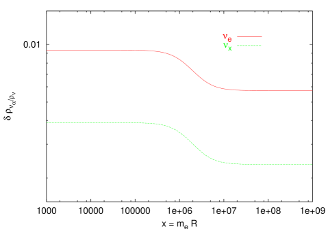
Figure 1: Evolution of $\delta\rho_{\nu_{\alpha}}(m_{\alpha})/\rho_{\nu_{\alpha}}^{0}(m_{\alpha})\,$, for a neutrino mass $m_{\alpha}=1\,$ eV (see text for further details).

In Figure 1, we plot $\delta\rho_{\nu_{\alpha}}(m_{\alpha})/\rho_{\nu_{\alpha}}^{0}(m_{\alpha})$ for the reference choice $m_{\alpha}=1$ eV, using the coefficients $c^{\alpha}_{i}$ of Table 2. The $x$ range corresponds to a variation of the temperature from $T\sim 1$ keV till $T\sim 10^{-3}$ eV. We see that the effect of incomplete decoupling and QED plasma masses for $e^{\pm}$ and $\gamma$ on neutrino energy density decreases as the temperature becomes comparable with the value of the neutrino mass. Notice that, from (29), at very low values of $T$, when the neutrino energy is dominated by the mass term, $\delta\rho_{\nu_{\alpha}}(m_{\alpha})/\rho^{0}_{\nu_{\alpha}}(m_{\alpha})$ reaches an asymptotic value, which is given by the change in the neutrino number density due to the above effects, normalized with the number density for a pure thermal Fermi-Dirac distribution.

5 Conclusion

In this paper we have considered how the two effects due to incomplete neutrino decoupling and QED corrections to the $e^{\pm}$ and photon plasma equation of state affect the effective neutrino degrees of freedom, a crucial parameter for many cosmological observables.

The main result of our analysis, which have been carried out by numerically solving the set of Boltzmann equations describing neutrino decoupling, is a value for $N_{\nu}^{\rm eff}=3.0395$, for the standard case of three active neutrino flavours. The issue is certainly not new, but we hope our study will contribute to reach a better accuracy in the theoretical determination of relativistic energy density of the Universe. In particular we have stressed that there is quite an interesting interplay between the two effects we have considered, so that at the level of accuracy of $0.005$ on $N_{\nu}^{\rm eff}$, their corrections to the neutrino energy density cannot be naively summed as they were fully independent.

We have also considered the less standard scenario of extra species contributing to $N_{\nu}^{\rm eff}$ , and how they affect the calculation of the thermal distortion of neutrino distribution, as well as the final value for photon temperature after the $e^{\pm}$ annihilation phase.

Despite of the smallness of the corrections we have been concerned with in this paper, nevertheless a careful analysis of data on the CMB anisotropy spectrum at large multipoles may be able in the near future to reveal their effects. Estimated sensitivity of Planck satellite experiment to relativistic energy density is at least of the order of $\Delta N_{\nu}^{\rm eff}\simeq 0.2$, but it is strongly improved, $\Delta N_{\nu}^{\rm eff}\simeq 0.005$ [22], when including polarization measurements and strong priors.

References

- [1] E.W. Kolb and M.S. Turner, The Early Universe (Addison-Wesley, 1990).
- [2] D.A. Dicus, E.W. Kolb, A.M. Gleeson, E.C. Sudarshan, V.L. Teplitz and M.S. Turner, Phys. Rev. D 26 (1982) 2694.
- [3] A.F. Heckler, Phys. Rev. D 49 (1994) 611.
- [4] V.F. Shvartsman, Pisma Zh. Eksp. Teor. Fiz. 9 (1969) 315 [JETP Lett. 9 (1969) 184].
- [5] G. Steigman, D.N. Schramm and J.R. Gunn, Phys. Lett. B 66 (1977) 202.
- [6] A.D. Dolgov, S.H. Hansen and D.V. Semikoz, Nucl. Phys. B 503 (1997) 426.
- [7] A.D. Dolgov, S.H. Hansen and D.V. Semikoz, Nucl. Phys. B 543 (1999) 269.
- [8] S. Esposito, G. Miele, S. Pastor, M. Peloso and O. Pisanti, Nucl. Phys. B 590 (2000) 539.
- [9] G. Steigman, astro-ph/0108148.
- [10] N.Y. Gnedin and O.Y. Gnedin, Astrophys. J. 509 (1998) 11.
- [11] B. D. Fields, S. Dodelson and M. S. Turner, Phys. Rev. D 47 (1993) 4309.
- [12] R.E. Lopez and M.S. Turner, Phys. Rev. D 59 (1999) 103502.
- [13] S. Esposito, G. Mangano, G. Miele and O. Pisanti, JHEP 0009 (2000) 038.
- [14] Y.I. Izotov and T.X. Thuan, Astrophys. J. 500 (1998) 188.
- [15] S. Hannestad, Phys. Rev. D 65 (2002) 083006.
- [16] R. Bowen, S.H. Hansen, A. Melchiorri, J. Silk, and R. Trotta, astro-ph/0110636.
- [17] S. Hannestad, Phys. Rev. Lett. 85 (2000) 4203.
- [18] M. Orito, T. Kajino, G.J. Mathews and R.N. Boyd, astro-ph/0005446.
- [19] S. Esposito, G. Mangano, A. Melchiorri, G. Miele and O. Pisanti, Phys. Rev. D 63 (2001) 043004.
- [20] J.P. Kneller, R.J. Scherrer, G. Steigman and T.P. Walker, Phys. Rev. D 64 (2001) 123506.
- [21] S. Hannestad, Phys. Rev. D 64 (2001) 083002.
- [22] R.E. Lopez, S. Dodelson, A. Heckler and M.S. Turner, Phys. Rev. Lett. 82 (1999) 3952.
- [23] U. Seljak and M. Zaldarriaga, Astrophys. J. 469 (1996) 437.
- [24] M.A. Herrera and S. Hacyan, Astrophys. J. 336 (1989) 539.
- [25] N.C. Rana and B. Mitra, Phys. Rev. D 44 (1991) 393.
- [26] S. Dodelson and M.S. Turner, Phys. Rev. D 46 (1992) 3372.
- [27] A.D. Dolgov and M. Fukugita, Phys. Rev. D 46 (1992) 5378.
- [28] S. Hannestad and J. Madsen, Phys. Rev. D 52 (1995) 1764.
- [29] N. Fornengo, C.W. Kim and J. Song, Phys. Rev. D 56 (1997) 5123.
- [30] S.H. Hansen, G. Mangano, A. Melchiorri, G. Miele, and O. Pisanti, Phys. Rev. D 65 (2002) 023511.
- [31] A.R. Zentner and T.P. Walker, Phys. Rev. D 65 (2002) 063506.
- [32] D.E. Groom et al. [Particle Data Group Collaboration], Eur. Phys. J. C 15 (2000) 1.