Probing the distribution of dark matter in the
Abell 901/902 supercluster with weak lensing

Abstract

We present a weak shear analysis of the Abell 901/902 supercluster, composed of three rich clusters at $z=0.16$. Using a deep $R$-band image from the $0.5^{\circ}\times 0.5^{\circ}$ MPG/ESO Wide Field Imager together with supplementary $B$-band observations, we build up a comprehensive picture of the light and mass distributions in this region. We find that, on average, the light from the early-type galaxies traces the dark matter fairly well, although one cluster is a notable exception to this rule. The clusters themselves exhibit a range of mass-to-light ($M/L$) ratios, X-ray properties, and galaxy populations. We attempt to model the relation between the total mass and the light from the early-type galaxies with a simple scale-independent linear biasing model. We find $M/L_{B}=130h$ for the early type galaxies with zero stochasticity, which, if taken at face value, would imply $\Omega_{m}<0.1$. However, this linear relation breaks down on small scales and on scales equivalent to the average cluster separation ($\sim$1 Mpc), demonstrating that a single $M/L$ ratio is not adequate to fully describe the mass-light relation in the supercluster. Rather, the scatter in $M/L$ ratios observed for the clusters supports a model incorporating non-linear biasing or stochastic processes. Finally, there is a clear detection of filamentary structure connecting two of the clusters, seen in both the galaxy and dark matter distributions, and we discuss the effects of cluster-cluster and cluster-filament interactions as a means to reconcile the disparate descriptions of the supercluster.

Accepted for publication in the Astrophysical Journal, November 10, 2001

1 Introduction

Gravitational lensing is a powerful tool that allows us to directly map dark matter and determine the relation between the observed distribution of light and the underlying mass distribution. In recent years, the development of sophisticated lensing techniques coupled with a new generation of wide-field imaging instruments has opened doors to lensing studies on unprecedentedly large scales. Weak lensing is now a well-established method for determining the mass distribution of rich clusters of galaxies (Bartelmann & Schneider, 2001; Mellier, 1999). With the increased confidence in lensing techniques, recent studies have turned from clusters to blank fields (Bacon et al., 2000; Kaiser et al., 2000; Van Waerbeke et al., 2000; Wittman et al., 2000; Maoli et al., 2001) to measure the statistical ‘cosmic shear’ due to lensing by large-scale structures.

Superclusters, comprising $\sim$2-10 clusters of galaxies, are the largest known systems of galaxies in the Universe (Vogeley et al., 1994) and represent a stepping-stone between rich clusters and large-scale structure. Clusters of clusters and associated filamentary structures in the galaxy distribution have been observed at low redshift through redshift surveys of the Corona Borealis, Shapley, and Perseus-Pisces superclusters (e.g. Small et al., 1997; Quintana et al., 1995; Postman et al., 1988). Recently, supercluster studies have been extended to intermediate redshifts with the weak lensing study of MS0302+16 at $z=0.4$ by Kaiser et al. (1998), and pushed to even higher redshifts with the optical detection of a $z\sim 0.91$ supercluster by Lubin et al. (2000).

Superclusters are invaluable testing grounds for theories of cosmology, the growth of structure, galaxy formation, and the nature of dark matter. The presence or absence of filamentary structure can be used to probe theories of structure formation (e.g. Cen et al., 1995). The degree of substructure is reflective of the universal matter density parameter, $\Omega_{m}$, (Richstone et al., 1992), and simulations find that the mass fraction in filaments is expected to be slightly larger in a low-density universe (Colberg et al., 1999). Furthermore, supercluster mass-to-light ratios ($M/L$) can be also be used to determine $\Omega_{m}$ (Kaiser et al., 1998). This latter calculation rests on the assumption that the supercluster $M/L$ ratio is representative of the Universe as a whole, i.e. that the $M/L$ ratio flattens to a constant on supercluster scales (Bahcall et al., 2000).

In this paper we present a weak lensing analysis of the Abell 901(a,b)/Abell 902 supercluster (referred to hereafter as A901/902) using the $0.5^{\circ}\times 0.5^{\circ}$ Wide-Field Imager (WFI; Baade et al., 1998, 1999) on the MPG/ESO 2.2m telescope. Our aim is to trace the dark matter distribution in the supercluster field and to investigate whether it is concentrated in cluster cores or distributed through filamentary structures. In the ‘Cosmic Web’ theory of structure formation (Bond et al., 1996), filaments emerge from the primordial density field after cluster formation. These filaments are thought to harbor a large fraction of present day baryons in the form of hot gas, prompting calls for X-ray searches (Pierre et al., 2000). However, attempts to detect filamentary X-ray gas have to date been unsuccessful, yielding only upper limits (e.g. Briel & Henry, 1995). As X-ray emissivity scales as the square of the density while gravitational shear scales linearly, a weak lensing-based approach may prove more successful in uncovering such structures. Kaiser et al. (1998) report tantalising but tentative evidence for a lensing detection of a mass bridge within MS0302+16. Here we will use weak shear reconstruction algorithms to create two-dimensional maps of the mass distribution and search for similar filamentary structures within the A901/902 supercluster region.

In addition, we also wish to determine how well the optical light traces the underlying dark matter, and how the cluster masses determined by weak lensing compare to those predicted from the results of a previous X-ray study of the region (Schindler, 2000). Finally, we wish to examine the ratio of the total mass of the system to the $B$-band light of the early-type supercluster galaxies, and to discuss the resulting implications for $\Omega_{m}$. Measurements of the mass-to-(total)-light ratio of clusters of galaxies typically yield values in the range $M/L\sim 200-300h$ (Carlberg et al., 1996; Mellier, 1999), which, if taken as the universal $M/L$, imply $\Omega_{m}=0.2$. However, if the $M/L$ ratio continues to increase with scale to the regime of superclusters or beyond, $\Omega_{m}$ could be considerably larger. This would require the galaxies to be significantly biased with respect to the mass, so that the efficiency of galaxy formation is greatly enhanced in the densest regions.

Bahcall, Lubin, & Dorman (1995) explore this hypothesis, and compile results from the literature to trace an increasing $M/L$ ratio as they proceed in scale from galaxies to groups and then to clusters. Their best-fit values for the $M/L$ of individual galaxies result in a $M/L$ ratio for ellipticals that is $\sim 4$ times that for spirals, suggesting that on average, ellipticals contain more mass than spirals for the same luminosity and radius. They conclude that the total mass of groups, clusters and superclusters can be accounted for by the mass of the dark halos of their member galaxies (which may have been stripped off in a dense environment but still remain within the system) plus the mass of the hot inter-cluster gas, and that there is no great repository of dark matter hidden on larger scales.

Indeed, on the scale of superclusters, measurements of galaxy velocity dispersions indicate that the universal $M/L$ function appears to flatten to $\sim 300h$ (assuming that the systems are bound but not necessarily in an equilibrium state). Bahcall et al. (1995) find little evidence that the $M/L$ ratio continues to increase with scale, implying $\Omega\sim 0.2$. The issue of a low supercluster $M/L$ ratio was revisited by Kaiser et al. (1998) in a weak-shear study of a supercluster of three X-ray luminous clusters at $z=0.4$. This was the first direct mapping of dark matter on these scales, independent of biasing assumptions. Kaiser et al. present the remarkable result that the light from the color-selected early-type galaxies alone is sufficient to trace the mass as revealed by weak lensing, with the mass no more extended than the early-type galaxies and with late-type galaxies having negligible $M/L_{B}$. Our weak lensing study affords us the opportunity to test this hypothesis on another supercluster system at lower redshift, and to determine if a single, scale-independent $M/L$ ratio can describe the relation between mass and light in the entire system. We will discuss the resulting implications of such a conclusion for values of $\Omega_{m}$, and explore other possible biasing relations.

1.1 The A901/902 supercluster

The A901/902 supercluster is composed of three clusters of galaxies, all at $z=0.16$ and lying within $30\arcmin\times 30\arcmin$ on the sky. Abell 901 is listed as a double cluster (A901a and A901b) with irregular morphology in the X-ray Brightest Abell-type Cluster Sample (XBACS; Ebeling et al., 1996) of the ROSAT All-Sky Survey, having $L_{X}$(0.1-2.4 keV)$=6.01$ and $3.49\times 10^{44}$ erg s^-1.

Pointed ROSAT HRI observations by Schindler (2000) reveal that the emission from the ‘brighter subcluster’ of Abell 901 (labelled Abell 901a in the Ebeling et al. nomenclature used in this paper) suffers from confusion with several X-ray point sources in the vicinity. She concludes that the X-ray emission from Abell 901a is in fact point-like and suggests emission from an active nucleus as a likely candidate for the source. Abell 901b, on the other hand, is shown to exhibit very regular and compact cluster emission, with a revised $L_{X}$(0.1-2.4 keV)$=3.6\pm 0.1\times 10^{44}$ erg s^-1, possibly containing a cooling flow. No X-ray flux is detected at the optical center of Abell 902 (as determined by Abell, Corwin, & Olowin, 1989), although there is point-like emission 2 arcmin to the west of this position.

Both the clustering of number counts (Abell et al., 1989) and the X-ray emission (Ebeling et al., 1996; Schindler, 2000) in this field indicate that this is an overdense region. How exactly mass is distributed through the field and which of the objects discussed here deserves to be labelled a ‘cluster’ is not so clear, however. We therefore turn to gravitational lensing to trace the underlying mass distribution of this system.

The structure of the paper is as follows: in $\S\ref{sec:obs}$ we outline the observations of the supercluster field and discuss the data reduction and astrometric issues. In $\S\ref{sec:psf}$ we perform the corrections for the point-spread function necessary to accurately measure the shapes of the background galaxies. In $\S\ref{sec:clusters}$ we discuss the photometric properties of the clusters, and in $\S\ref{sec:lensing}$ we present the results of the weak lensing analysis. $\S\ref{sec:xcorr}$ contains a statistical cross-correlation of the light and mass distributions. Finally, in $\S\ref{sec:discussion}$ we summarize the results and present our conclusions.

2 Observations and Data Reduction

2.1 Observing strategy

The observations presented in this paper were undertaken as part of the COMBO-17 survey (Wolf et al., 2001). The survey has imaged one square degree of sky split over four fields using the Wide-Field Imager (WFI) at the MPG/ESO 2.2m telescope on La Silla, Chile. For lensing studies, one of the fields was centered on the A901/A902 supercluster. The filter set was chosen such as to provide reliable classification and photometric redshift estimators, and consists of five broad-band filters ($UBVRI$) and 12 narrow-band filters ranging from 420 to 914 nm. A deep $R$-band image taken under the best seeing conditions during each run provides excellent data for gravitational lensing studies.

In §2.2, we outline the initial processing applied to images under the standard WFI pipeline reduction developed at the MPIA Heidelberg. Although the resulting images are adequate for almost all astrophysical applications, we need further higher-order corrections for the detection of unbiased lensing shear. This is described in §2.3.

The data used in this paper are the deep $R$-band and supplementary $B$-band images from the COMBO-17 observations of the supercluster field. We will use the $R$-band image for a weak shear analysis of the supercluster, in combination with color information from the bluer band to separate foreground and background galaxy populations. The details of the observations are presented in Table 2.1. The discussion of the full 17 filter dataset for the A901/902 field and the photometric redshifts derived from it is reserved for a further paper.

Table 1

Summary of Observations Used for the Present Study

Date	Filter	Exposures		Date	Filter	Exposures
1999 Feb 18	B	10$\times$500 s		2000 Jan 31	R	8$\times$600 s
1999 Feb 19	B	12$\times$500 s		2000 Feb 06	R	27$\times$500 s
				2000 Feb 12	R	9$\times$500 s
	total:	3.05 h			total:	6.33 h

2.2 Initial processing by standard WFI pipeline

Imaging by the Wide Field Imager (WFI) on the 2.2m telescope at La Silla, Chile is carried out with a $4\times 2$ array of $2048\times 4096$ pixel CCDs. For clarity and ease of reference, chips are labelled by the letters ‘a’, starting at the top left of the mosaic, through a clockwise direction to chip ‘h’ located at the bottom left of the mosaic. With a vertical chip-to-chip separation of 59 pixels and a corresponding horizontal separation of 98 pixels, the scale of 1 pix $\equiv 0.238^{\prime\prime}$ gives a total field of view (FOV) for the WFI of $0.56^{\circ}\times 0.55^{\circ}$.

De-biasing is conducted by individually subtracting the (vertically smoothed) level measured in the overscan region of each chip image. Non-linearity (i.e. departure from the proportionality between the number of incident photons and the electric charge read out at the end of an exposure, which worsens with increasing intensity), is corrected by scaling each de-biassed chip image according to an ESO laboratory-determined factor (Baade, 1999). Only chips b, c, f & g need be corrected in this way, the worst non-linearity being exhibited by chip f which at saturation (65000 counts) deviates by $1.4\%$ from linearity.

Production of mosaiced images must be handled with care due to the physical complication of chip-to-chip misalignments in the CCD array. Translational misalignments are easily accommodated, however intrinsic chip rotations with respect to the array are not. A slight chip rotation produces the added complexity of having to rotate the chip image before insertion into the mosaic.

Rather than rebin images, rotations are approximated by dividing up the misaligned chip images into horizontal strips. Each strip is then inserted into a temporary chip image with a horizontal offset determined by the required rotation. This temporary chip image is then divided into vertical strips and then finally inserted into the mosaic with vertical offsets according to the rotation. Adopting this shearing method considerably reduces data reduction time, is optimal for cosmic ray removal (see below), and has been shown to have no effect on photometry. Table 2 lists chip rotations determined independently in this work as part of the astrometric fitting described in §2.3.1, although they are in agreement with the rotations incorporated in the WFI pipeline.

After producing mosaic images in this fashion, science frames were flattened with normalized mosaic flat-field frames produced in exactly the same way. Since each physical pixel is maintained intact throughout the reduction process, cosmic ray hits and cosmetic chip defects can be detected very efficiently by comparing dithered images taken through the same filter. To this end, flat-field corrected mosaic images are aligned with respect to moderately bright stars in the field (to integer pixel accuracy). The cosmic ray detection algorithm employs a $\sigma$-clipping with respect to the median pixel value derived from at least five exposures with comparable seeing. Discrepant values are replaced by the median value.

2.3 Astrometry

2.3.1 Linear astrometric fitting

While the creation of mosaiced images by the standard reduction pipeline described above is sufficient for most purposes, we require a more rigorous characterization of the geometry of the camera for our weak shear study. For example, intrinsic rotation of the FOV of the WFI is known to be caused by imperfect alignment of the 2.2m telescope axis of rotation with the celestial pole as well as telescope flexure in tracking across the sky. Other causes are atmospheric in origin, due to the differential refraction of object images by the Earth’s atmosphere and the fact that an offset in right ascension produces a rotation due to the non-perpendicularity of lines of declination away from the celestial equator.

To this end, we chose to treat each CCD image as an individual contribution to the final coadded image, and to compute an astrometric solution separately for each chip image. For each debiased, normalized, flattened and cosmic-ray cleaned mosaic the approximate rotations described above were removed to restore the original detector coordinate system. Next, the eight component chip images were extracted from each mosaic. Henceforth the term ‘image’ shall refer to an individual 2K$\times$4K chip image.

Using SExtractor 2.1 (Bertin & Arnouts, 1996) an initial catalogue of bright objects was created for each image. A rough transformation was performed to convert the pixel coordinates ($x,y$) to celestial coordinates ($\alpha,\delta$) using the pointing information encoded in the image header. The objects in the catalogue were then matched to the SuperCOSMOS Southern Sky Survey within a tolerance of 5″. These reference objects were used to iteratively calculate a linear astrometric solution for the image, with the tangent point for projection being the optical axis. The rms residuals of the objects used in the final solution (typically numbering $\sim$400 per image) differed from the median by less than 3$\sigma$.

The linear fit used takes the form:

$$\begin{array}[]{rcl}x&=&a_{0}+a_{1}\xi+a_{2}\eta\\ y&=&a_{3}+a_{4}\xi+a_{5}\eta,\end{array}$$ (1)

where the ‘expected’ coordinates (standard coordinates on the tangent plane, projected about the optical axis) are related to the ‘measured’ coordinates (x-y coordinates on the detector plane) by a 6 coefficient linear fit. Note that field-to-field variations were found to be significant, so the external calibration was calculated for each image individually.

The linear fit can be decomposed into terms such as pixel scale, rotation, and non-perpendicularity of the coordinate axes for each image. The average rotation angles required to align the x-y axes to a N-E orientation and the angle of deviation from the perpendicular for the x-y axes are listed in Table 2.3.1 for each chip. The resulting fits produced median rms residuals of 0.2 arcsec, i.e. less than 1 pixel and close to the limiting accuracy of the photographic data.

Table 2

Decomposition of the Astrometric Fits

	Linear Fit						Radial Fit
Chip	Rotation		$\pm$	Skew	$\pm$		$C$
a	-288.	3	53.5	-104.5	21.4		6.	4
b	276.	0	54.0	-117.0	17.2		-38.	7
c	126.	0	53.2	120.1	20.2		-29.	4
d	130.	7	54.5	161.9	19.8		0.	7
e	144.	9	53.9	-157.3	11.6		1.	6
f	123.	8	53.0	-115.2	16.3		-39.	8
g	120.	9	53.5	104.8	24.4		-50.	6
h	-98.	3	49.9	74.7	27.2		13.	0

2.3.2 Quantifying shear induced by radial distortions

While the linear fits produced satisfactory results, it is nevertheless important to consider higher-order or radial distortions. As a test to search for pincushion or barrel distortions, a radial distortion term was added to the linear fit, of the form:

$$r^{\prime}=r(1+Cr^{2}),$$ (2)

where $r$ is the radial distance from the tangent point (optical axis), $c$ is the distortion coefficient, and $r^{\prime}$ is the radial distance from the tangent point in the presence of the distortion.

The fit for some chips (particularly the y-component of the fit for the inner four chips) improved somewhat when the radial term was added, but there was no significant improvement in the resulting rms residuals for the instrument as a whole. However, the results of the radial fitting do allow us to constrain the amount of linear distortion found in each chip. The resulting values of $C$ (listed in the final column Table 2.3.1) were small, and had a small dispersion for each chip from image to image. The contrast between the values for the inner and outer four chips indicates that the mosaic as a whole does not display a typical radial distortion pattern.

Knowing the distance of the edge of each chip from the tangent point, this yields distortions of $\delta r/r\sim 0.025$% at the furthest corners of the camera, or slightly higher for the inner chips. This tallies well with the figures quoted in the WFI manual, which claims geometric distortions $\leq$0.08% across the entire camera.

We can further quantify any artificial shear induced by such a radial distortion using the relations of Bacon et al. (2000). If the displacement $\delta{\bf r}=Cr^{3}$ and ${\bf\hat{r}}$ is the unit radial vector, then the induced instrumental shear is $\gamma_{i}=Cr^{2}\hat{e}_{i}$, where $\hat{e}_{i}$ is the unit radial ellipticity vector. Using the radial distortion coefficients derived from our astrometric fits, we find a shear pattern with amplitude $\gamma<0.0001$ throughout.

It is quite clear that despite the wide field of view of the camera, the instrumental distortion in the WFI is extremely small and will not significantly affect our shear measurements. We shall continue with the analysis using the simple linear fit with no correction for the negligible radial distortion. Note that corrections involving higher-order polynomials could be used to remove any non-linear, non-radial distortions present, but we see little evidence of these from the residuals following the linear fit.

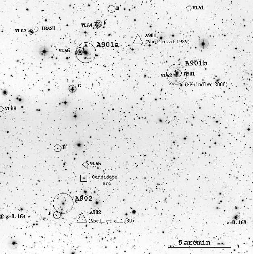
Figure 1: The $R$-band view of the central $20\times 20$ arcmin of the supercluster field (seen at reduced resolution). The two large triangles mark the positions of Abell 901 and Abell 902 in the original catalogue of galaxy clusters (Abell et al., 1989), while the three large circles indicate the optical centers of the clusters that we have adopted in this paper. The smaller circles indicate the locations of the ROSAT/HRI X-ray sources from Schindler (2000). The remaining objects marked by diamonds are two galaxies with known redshift (also from Schindler, 2000), radio detections from the NRAO/VLA All Sky Survey (Condon et al., 1998, labelled ‘VLA’) and the IRAS Faint Source Catalogue (Moshir, 1990, labelled ‘IRAS’). North is up, east is to the left.

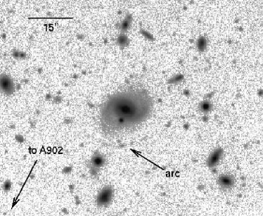
Figure 2: Candidate giant arc. The potential deflecting galaxy is a barred spiral with $R=18$ and is located $\sim$2.5 arcmin from the center of Abell 902.

2.3.3 Registration and coaddition

The linear astrometric fits for each individual chip image were used to register the images to the same coordinate system. The images were thus aligned and combined with 3$\sigma$ clipping rejection of bad pixels, scaling by the median and weighting by exposure time. Due to the large number of images contributing to each pixel in the final image (44 for the $R$-band, 22 for the $B$-band), most bad columns and pixels were removed by the $\sigma$-clipping algorithm. The combined mosaiced images were trimmed of the noisy outlying regions where the overlap from the dithering pattern was not complete. The resulting final images used for the weak shear analysis measured $8192\times 8192$ pixels ($32.5\arcmin\times 32.5\arcmin$), and the measured seeing was 0.7″  ($R$-band) and 1.1″  ($B$-band).

Fig. 1 shows the inner regions of the $R$-band image, along with the published positions of the clusters from Abell et al. (1989) and the X-ray sources from Schindler (2000). In addition, Fig. 2 shows a candidate strongly lensed source. The arc-like structure is located 13 arcsec from a bright barred spiral galaxy, which is in turn located $\sim$2.5 arcmin from the adopted center of Abell 902. The deflecting galaxy has $R=18$ and $B-R$ color similar to the cluster galaxies.

2.4 Photometric calibration

Photometric calibration was provided from two spectrophotometric COMBO-17 standards (Wolf et al., 2001, see) in the A901/902 field selected from the spectral database of the Hamburg/ESO (HE) Survey (Wisotzki et al., 2000). Spectra were obtained using a wide ($5\arcsec$) slit on the ESO/Danish 1.54m and the ESO 1.52m telescope at La Silla in November 2000. Correcting the observed A901/902 standard spectra to remove the instrument, optics and atmosphere signature, photometric scalings were determined from the HE survey standards. Using the $B$- and $R$-band WFI filter responses, zero points were calculated and magnitudes transformed to the Vega system. Apparent magnitudes were corrected for extinction using the IRAS dust maps of Schlegel et al. (1998). For an average $E(B-V)=0.058$ and assuming an $R_{V}=3.1$ extinction curve, we derive corrections $\Delta m_{B}=0.25$ and $\Delta m_{R}=0.16$. We estimate that the $S/N=3$ limiting magnitude in the two bands is $R=25.7$ and $B=25.5$.

3 Point spread function corrections

In this section we outline the correction for such effects as variable seeing conditions from exposure to exposure, telescope tracking errors, as well as smearing of objects due to imperfect alignment of images before coaddition and the circularization of small objects by the seeing. These corrections have been discussed in detail in several previous papers (Kaiser, Squires, & Broadhurst, 1995, hereafter KSB, with refinements in Luppino & Kaiser 1997 and Hoekstra et al. 1998).

3.1 Object catalogues

The imcat software described in Kaiser et al. (1999) was used to determine the shape parameters for the faint galaxy sample used in the weak lensing analysis. For ease of computing, the hfindpeaks object detection routine was performed on 2K$\times$2K image sections, and the resulting catalogues shifted by the appropriate amount and concatenated together. The local sky background was estimated using getsky and and aperture magnitudes and half-light radii, $r_{h}$, for each object were calculated using the apphot routine. Finally, getshapes was used to calculate the weighted quadrupole moments, defined as

$$I_{ij}\equiv\int d^{2}x\ w(x)x_{i}x_{j}I(x),$$ (3)

where $I(x)$ is the surface brightness of the object at angular position $x$ from the object center, and $w(x)$ is a Gaussian weight function. The scale length, $r_{g}$, of the weight function is previously determined by hfindpeaks as the radius of the Mexican hat filter function that maximizes the signal-to-noise of the object detection. Finally, the weighted quadrupole moments are used to calculate the ellipticity components

$$e_{1}=\frac{I_{11}-I_{22}}{I_{11}+I_{22}},\hskip 28.45274pte_{2}=\frac{2I_{21}}{I_{11}+I_{22}}.$$ (4)

Photometric catalogues were also constructed for each image, using SExtractor 2.1. The detection criteria were defined such that an object was required to be $1.5\sigma$ above the background and comprising at least 7 connected pixels. The photometric information (from SExtractor) and the shape estimates (from imcat) were then merged to provide the final catalogue for lensing analysis, conservatively requiring that an object be detected by both software packages. Due to the superior seeing and longer exposure time, the shape parameters derived from the $R$-band image will be used for the weak shear reconstructions, although as we describe in $\S\ref{sec-col}$, the $B-R$ colors will be used to discriminate between the foreground (including the cluster galaxies) and the background populations.

Finally, a mask was created directly from the image to remove objects from the catalogue that lay in areas contaminated by bright stars, ghost images, and diffraction spikes. This masked region totalled only 3.4% of the total area of the image, and can be seen in Fig. 6.

3.2 Anisotropic PSF correction

Fig. 3 shows the size-magnitude diagram for the full sample of objects. The stars are clearly visible as a column of objects with half-light radii of 1.8 pixels, and can be distinguished from galaxies down to $R\sim 23$. To examine the behavior of the point-spread function (PSF) across the image we select a sample of non-saturated ($R>16$) stars.

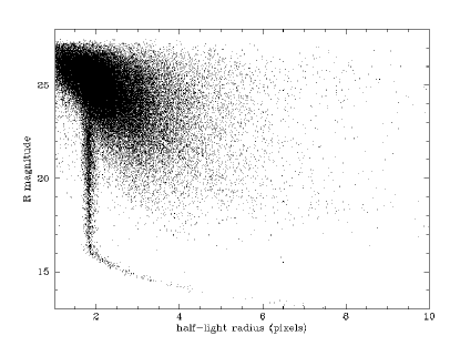
Figure 3: Magnitude vs. half-light radius of all objects in the initial $R$-band catalogue. Stars form a clear vertical locus and can be easily differentiated from galaxies down to $R\sim 23$. Saturated stars deviate from this column towards larger half-light radii at bright magnitudes.

The stellar ellipticity pattern across the final summed $R$-band image is shown in Fig. 4, and the distribution of ellipticities in Fig. 5. While there is overlap between the chip regions due to the dithering pattern, we divide the mosaiced image into 8 approximate chip regions for the purposes of the PSF correction. Within these regions, outlined in Fig. 4, the PSF is smoothly varying and even within the overlap regions there are no sharp discontinuities in the behavior of the PSF.

Figure 4: Ellipticity pattern of stars on the $R$-band coadded image, before (left) and after (right) correction for the anisotropic PSF. The horizontal and vertical lines show the approximate chip divisions used for the polynomial fitting.

Figure 5: Ellipticities distribution of stars, before (crosses) and after (dots) correction for PSF anisotropies.

We apply preliminary cuts to our catalogue to exclude objects unsuitable for shear analysis. We remove those objects with a half-light radius smaller than the stellar half-light radius, as well as objects with an imcat significance $\nu<5$ and with ellipticity $e>0.5$. Next, within each chip region we fitted a two-dimensional cubic to the measured stellar ellipticities, iterating twice to remove outliers with large residuals.

The modelled stellar ellipticities were used to correct the ellipticities of the galaxies by

$$e_{\rm corr}=e-\frac{P_{\rm sm}}{P_{\rm sm}^{*}}e^{*},$$ (5)

where starred quantities referred to stellar properties, and $P_{\rm sm}$ is the imcat ‘smear polarizability’ matrix of higher moments of surface brightness described in KSB. As the non-diagonal elements are small ($<2\times 10^{-4}$) and the diagonal elements nearly equal, we choose to treat this as a scalar equal to half the trace. The mean stellar ellipticity before correction and after correction was then

$$\begin{array}[]{llc}e_{1}=0.014\pm 0.011&e_{2}=-0.047\pm 0.014&{\rm(before)}\\ e_{1}=0.00013\pm 0.006&e_{2}=0.00003\pm 0.006&{\rm(after)}.\end{array}$$

Fig. 4 and Fig. 5 show the resulting pattern and distribution of corrected stellar ellipticities.

3.3 Isotropic PSF correction

The isotropic correction recovers the lensing shear prior to circularization by the PSF. Following Luppino & Kaiser (1997) and Hoekstra et al. (1998) we use the corrected galaxy ellipticities in conjunction with the ‘shear polarizability’ tensor $P_{\rm sh}$ to calculate the shear estimate

$$\gamma=P^{-1}_{\gamma}e_{\rm corr},$$ (6)

where

$$P_{\gamma}=P_{\rm sh}-\frac{P_{\rm sh}^{*}}{P_{\rm sm}^{*}}P_{\rm sm}.$$ (7)

Again, the starred quantities refer to stellar properties, and $P_{\rm sh}^{*}$ and $P_{\rm sm}^{*}$ are treated as scalars equal to half the trace of the respective matrices. To calculate $P_{\gamma}$ for the galaxies, we fit $P^{11}_{\gamma}$ and $P^{22}_{\gamma}$ as a function of smoothing radius $r_{g}$, and insert the fitted value into equation (6) to calculate the shear measurement for each galaxy. Finally, we remove from the catalogue any galaxies with a resulting $|\gamma|>2$ due to noise. Note that this procedure actually yields the reduced shear, $\gamma/(1-\kappa)$, but in the wide-field, weak lensing limit ($\kappa\ll 1,\gamma\ll 1$) in which we are working this reduces to the shear, $\gamma$.

4 Cluster properties

To identify the likely members of the supercluster, we first spatially separate the catalogue of galaxies. We then use the resulting samples to isolate the tight sequence of early-type supercluster galaxies on the $B-R$ vs. $R$ color-magnitude diagram.

Fig. 6 shows the locations of all the objects in the catalogue within the $32.5\arcmin\times 32.5\arcmin$ field of view. The large circles represent an aperture of radius 4.6 arcmin around each cluster. The angular size scales as

$$R(\theta)=0.87D_{A}(z_{L})(\theta/1^{\prime})h^{-1}{\rm Mpc}$$ (8)

where the dimensionless angular distance

$$D_{A}(z) = \frac{1}{(1+z)}\int^{z}\frac{dz}{[\Omega_{m}(1+z)^{3}+\Omega_{\Lambda}]^{1/2}},$$ (9)

$$\simeq \frac{z}{(1+z)(1+3/4\Omega_{m}z)}$$ (10)

and the second line is a good approximation to the low-redshift angular distance in a spatially flat model with cosmological constant. For our supercluster at $z=0.16$ this is relatively insensitive to cosmology, and yields

$$R(\theta) = 0.11(\theta/1^{\prime})h^{-1}{\rm Mpc}$$ (11)

$$= 0.002(\theta/1^{\prime\prime})h^{-1}{\rm Mpc}.$$ (12)

Thus the radii of the apertures in Fig. 6 correspond to 0.5$h^{-1}$ Mpc at the redshift of the supercluster.

Table 5.2.1 lists the coordinates chosen as the center of each of the three clusters: in Abell 901a and 901b this corresponded to the obvious brightest cluster galaxy of (close to the X-ray positions of Schindler, 2000), and in Abell 902 the more northern of the two bright galaxies in the center of overdensity of numbers in that region. Note that these three positions differ slightly from the (two) positions given in Abell et al. (1989) for Abell 901 and Abell 902 (see Fig 1).

An attempt to quantify the richness of each of the three clusters is hampered by their close proximity. The original Abell richness class (Abell, 1958) is determined from the number of galaxies in the magnitude range $m_{3}$ to $m_{3}+2$ (where $m_{3}$ is the magnitude of the third brightest cluster galaxy) contained within a 1.5$h^{-1}$ Mpc radius. In the case of the A901/902 supercluster, the maximum separation between Abell 901a and Abell 902 is only 7.8 arcmin, or $\sim$850 $h^{-1}$ kpc at $z=0.16$. We can therefore at best place a lower limit on the Abell richness class by considering the counts within a 3.9 arcmin radius. This yields $N_{\rm Abell}=34,27,$ and $20$ galaxies for A901a, A901b, and A902, respectively, which corresponds to an Abell richness class 0 in each case. More informative, however, is to consider the supercluster as a single system. In this case we can probe the entire $R_{\rm Abell}=1.5h^{-1}$ Mpc (measuring from the centroid of the cluster positions) and find $N_{\rm Abell}$ = 92, corresponding to an Abell richness class II.

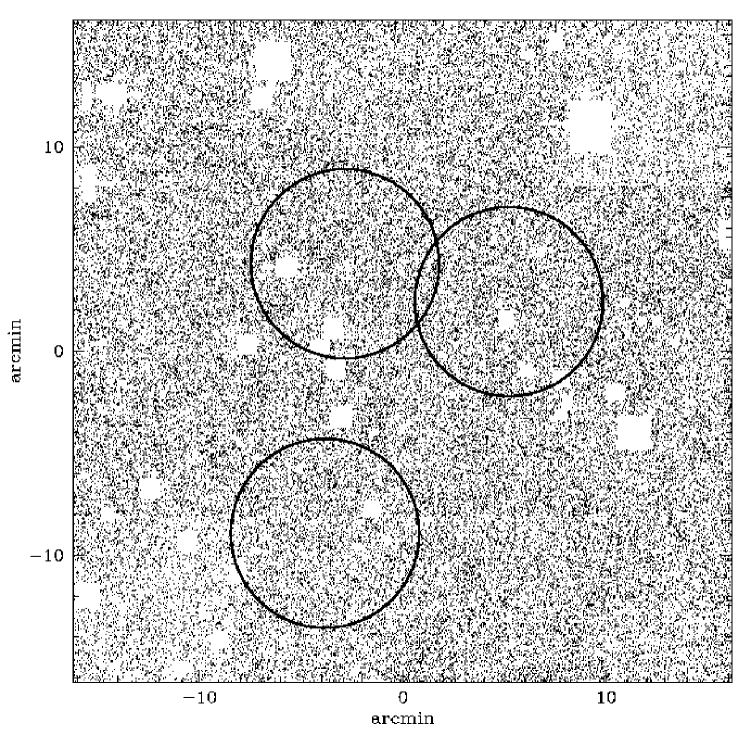
Figure 6: Division of catalogue into ‘cluster’ and ‘field’ regions. Each dot represents one galaxy in the catalogue, with the area masked out due to contamination by bright stars and diffraction spikes indicated by the blank rectangular regions. The circles are apertures of radius 4.6 arcmin (500$h^{-1}$ kpc) around the optical center of each cluster and define the ‘cluster’ regions used to isolate the color-magnitude sequence of supercluster galaxies (cf. Fig. 7 and Fig. 8).

4.1 Color selection of early type galaxies

Dividing the catalogue spatially into ‘cluster’ and ‘field’ regions according to boundaries shown in Fig. 6, we plot the $R$-band number counts in Fig. 7. A clear excess xof bright galaxies in the cluster region is visible. The $B-R$ vs. $R$ color-magnitude diagrams for the two regions (Fig. 8) reveal a prominent sequence of red galaxies with small scatter in the region of the clusters. We fit this relation according to

$$\left|B-R-(-0.0385R+2.21)\right|<0.1$$ (13)

and will use this color-cut to separate the supercluster members from the foreground and background population throughout the whole field of view, using the entire catalogue of galaxies.

Figure 7: Number-magnitude relation for ‘cluster’ and ‘field’ regions as defined in Fig. 6. A clear excess of bright galaxies in the cluster apertures is visible up to $R\sim 22$.

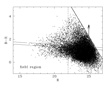
Figure 8: The $B-R$ vs. $R$ color-magnitude diagrams for the ‘field’ region (left) and the ‘cluster’ region (right) as defined by the boundaries in Fig. 6. The early-type cluster galaxies are clearly visible as a tight red sequence in the right-hand plot. The color selection criteria (eq. [13]) used to isolate the supercluster galaxies is shown by the parallel lines. Due to the relative shallowness of the $B$-band image with respect to the deep $R$-band image, approximately half the galaxies in each sample are detected in the $R$-band alone. The lower limit on the resulting $B-R$ color for these galaxies is indicated by the thick line and arrow. The dashed line at $R=22$ serves to further subdivide the populations into ‘bright’ and ‘faint’ samples.

Fig. 9 shows the result of this color cut when it is applied to the entire catalogue. The left panel shows the distribution of all the bright $(R<20)$ galaxies in the field, and the prominent clustering present is clearly visible. When the color-cut of equation (13) is applied, the structure of the supercluster as traced by the early-type galaxies is revealed. The distribution of these color-selected galaxies is shown in the right panel of Fig. 9. The three clusters, sharing the same color-magnitude relation for their early-type galaxies, are clearly present. Furthermore, the larger supercluster structure becomes clear (including galaxies stretching between the clusters, and an obvious sub-clump of supercluster galaxies approximately 12 arcmin west of Abell 902). This excess of supercluster galaxies outside the cluster boundaries defined by the apertures above accounts for a similar (but much weaker) color-sequence also visible in the color-magnitude diagram for the ‘field’ sample (left-hand side of Fig. 8).

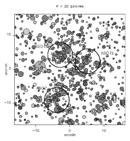
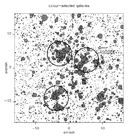
Figure 9: Spatial distribution of galaxies. Left: Position of all bright galaxies with $R<20$ in the supercluster field. The area of the symbol is proportional to the flux of the galaxy and a darker shade indicates a redder $B-R$ color. The large circles mark the optical centers of the three Abell clusters as in Fig. 6. Right: The same, but restricted to candidate supercluster members selected from the color-magnitude diagram (Fig. 8). This reveals not only that the three main clusters have similar colors (indicating similar redshifts) but also that the structure traced by the color-selected galaxies extends further afield. North is up, east is to the left.

4.2 Fraction of blue cluster members

An examination of the $R$-band image (Fig. 1) reveals that the three clusters are very different in morphological appearance. A901a most resembles the traditional picture of a relaxed cluster dominated by a central bright elliptical galaxy. A901b also contains a giant elliptical but the nearby cluster galaxies trace a more amorphous shape that appears to bleed into the middle of the supercluster (Fig. 9, left). This is at odds with the regular, compact X-ray emission detected by Schindler (2000). Finally, A902 is the most irregular of the three, with no well-defined center. It is interesting, however, that Fig. 1 clearly shows a prominent excess of bright, disky galaxies surrounding this cluster (absent from the vicinities of the other two).

To better understand the galaxy populations that make up these galaxy clusters, we calculate the fraction of bright galaxies too blue to survive the color selection but which may still be cluster members (presumably late-types). Taking a 4 arcmin radius aperture, we count those galaxies with $B-R$ bluer than the cluster sequence of equation (13) and compare with the total number of galaxies within the aperture for a given magnitude limit. We correct these numbers for background contamination using the number density of similarly selected galaxies in the complementary ‘field’ region, taking into account the area obscured by the mask.

Table 3

Fraction of Blue Galaxies for Various Limiting Magnitudes

$R<22$
Cluster	$N_{\rm blue,clus}$	$N_{\rm tot,clus}$	$N_{\rm blue,back}$	$N_{\rm tot,back}$	$f_{b}$
A901a	127	291	82.4	158.2	0.33
A901b	89	234	87.5	168.0	0.02
A902	137	302	89.6	172.0	0.36
$R<21$
Cluster	$N_{\rm blue,clus}$	$N_{\rm tot,clus}$	$N_{\rm blue,back}$	$N_{\rm tot,back}$	$f_{b}$
A901a	67	159	38.4	74.4	0.33
A901b	49	120	40.8	79.0	0.20
A902	69	154	41.7	80.9	0.37
$R<20$
Cluster	$N_{\rm blue,clus}$	$N_{\rm tot,clus}$	$N_{\rm blue,back}$	$N_{\rm tot,back}$	$f_{b}$
A901a	33	89	17.3	33.7	0.28
A901b	29	66	18.4	35.8	0.35
A902	38	81	18.8	36.6	0.43
$R<19$
Cluster	$N_{\rm blue,clus}$	$N_{\rm tot,clus}$	$N_{\rm blue,back}$	$N_{\rm tot,back}$	$f_{b}$
A901a	15	42	7.0	13.6	0.28
A901b	10	29	7.4	14.4	0.17
A902	16	29	7.6	14.8	0.58

We then calculate the fraction of bright blue galaxies within the clusters:

$$f_{b}=\frac{N_{\rm blue,cluster}-N_{\rm blue,background}}{N_{\rm total,cluster}-N_{\rm total,background}}.$$ (14)

The results tabulated in Table 4.2 confirm that A902 has a much higher $f_{b}$ than the other two clusters for a variety of magnitude limits, ranging as high as $f_{b}=0.58$ for $R<19$. We shall return to the issue of varying cluster luminosities when discussing cluster $M/L$ ratios in §6.

5 Weak shear analysis

5.1 Selection of background population

The observed tangential distortion of the background galaxies allows us to reconstruct the dimensionless surface density of the intervening matter, $\kappa=\Sigma/\Sigma_{{\rm crit}}$, where

$$\Sigma_{{\rm crit}}=\frac{c^{2}}{4\pi GD_{d}}\frac{D_{s}}{D_{ds}}$$ (15)

is the critical surface mass density. To turn the observed $\kappa$ into physical quantities requires knowledge of the angular diameter distances to the source and lens ($D_{d},D_{s}$), and the relative distance between the two ($D_{ds}$). In the case of weak lensing by a cluster of galaxies, the strength of the lensing signal is governed by the redshift distribution of the background sources. This information can be expressed by the parameter $\beta$, such that

$$\beta=\left<\frac{D_{ds}}{D_{s}}\right>_{z_{s}},\ D_{ds}\geq 0.$$ (16)

The galaxies we will use for our mass reconstructions will be composed for the most part of faint ($R>22$) galaxies or subsets thereof. It is of great importance, therefore, that we are able to determine the appropriate value of $\beta$ to use. Fig. 10a shows the dependence of the $\beta$ parameter on the redshift of the background sources, for a lens at $z=0.16$. Unlike lenses at higher redshift (see Hoekstra et al., 2000; Clowe et al., 2000), the relatively low redshift of our supercluster means that for $z_{s}\mathbin{\lower 3.0pt\hbox{$\hbox to0.0pt{\raise 5.0pt\hbox{$\char 62\relax$}\hss}\mathchar 29208\relax$}}1$, $\beta$ is relatively insensitive to the source redshift, regardless of the cosmological model used.

Figure 10: Dependence of the $\beta$ parameter on the redshift of the background sources, for a lens at $z=0.16$. Note that the relatively low redshift of the lens makes it much less sensitive to the redshift of the background sources for $\langle z_{s}\rangle\lower 2.15277pt\hbox{$\;\buildrel>\over{\sim}\;$}1$.

The CalTech Faint Galaxy Redshift Survey (CTFGRS; Cohen et al., 2000) is a survey in the direction of the Hubble Deep Field North containing redshifts for 671 galaxies. To the limits of our observations ($R\sim 26$) the median redshift of the CTFGRS implies that the median redshift of the background galaxies used in our lensing analysis will be greater than unity. We therefore adopt the value $\beta=0.8$, which corresponds to a single screen of background galaxies at $z_{s}=1.5$ (for an Einstein-de Sitter cosmology) or $z_{s}=1.0$ (for $\Omega_{m}=0.3,\Omega_{\Lambda}=0.7$).

5.2 Tangential shear

To measure the weak shear signal from the supercluster, we first calculate the tangential shear in radial bins around each of the three clusters, $\gamma_{T}=-(\gamma_{1}\cos 2\phi+\gamma_{2}\sin 2\phi)$. Here $\phi$ is the azimuthal angle from the center of the mass distribution, which we take as the optical center (see Table 5.2.1). To measure the radial surface profiles of the clusters we use the statistic (Fahlman et al., 1994):

$$\zeta^{\rm obs}(r,r_{\rm max})=\frac{2}{1-(r/r_{\rm max})^{2}}\int^{r_{\rm max}}_{r}d\ln(r)\langle\gamma_{T}\rangle.$$ (17)

This provides a lower bound on the surface mass density interior to radius $r$ relative to the mean surface density in an annulus from $r$ to $r_{\rm max}$:

$$\zeta(r,r_{\rm max})=\bar{\kappa}(<r^{\prime})-\bar{\kappa}(r<r^{\prime}<r_{\rm max}).$$ (18)

Figure 11: Radial cluster properties. Top: Tangential shear profiles as a function of radius from the optical center of clusters A901a (left), A901b (center), A902 (right). Errorbars are calculated from the variance in the orthogonal component of the shear (cf. Luppino & Kaiser, 1997). Middle: The corresponding $\zeta$ profile for each cluster, with uncertainties derived from the uncertainties in the tangential shear. Bottom: Lower bound on the enclosed mass within a radius $r$ for each cluster. In each case the solid line corresponds to the profile expected for a singular isothermal sphere, fit for each cluster to the observed tangential shear in radial bins (top row).

In Fig. 11 we show the tangential distortion of the faint ($R>22$) galaxies as a function of distance from the optical center for each of the three clusters: A901a, A901b, and A902. Non-zero tangential shear is observed in each case out to a significant radius.

To model the mass of each cluster, we fit a singular isothermal sphere to the observed tangential distortions. The best-fit models yield velocity dispersions $\sigma_{v}=542^{+195}_{-333}$, $659^{+129}_{-161}$, and $738^{+244}_{-384}$ km s^-1 for A901a, A901b, and A902 respectively. The fits to the tangential shear profiles are shown in the top panels of Fig. 11. Also shown in the central panels of Fig. 11 is $\zeta(r)$ for each cluster (note that the points are not independent as each depends on the mass profile of the cluster exterior to $r$). A value of $r_{\rm max}=500$ arcsec was used.

The A901a cluster, while shown by Schindler (2000) to be not as X-ray luminous as A901b is certainly the most regular ‘looking’ cluster of the three. It appears to have a regular and relaxed morphology with a prominent central bright elliptical galaxy. However, the tangential shear profile is significantly inconsistent with that expected for an isothermal sphere. The strong shear signal measured in the inner annuli ($80\arcsec<r<200\arcsec$) drops dramatically at larger radii, resulting in a $\zeta$ profile considerably steeper than isothermal. The sudden drop in signal could perhaps be explained by an encroachment into the neighboring cluster A901b (although the profile for that cluster shows no similar truncation).

The integral of the $\zeta$ statistic gives a lower bound on the mass enclosed within a radius $r$, $M(<r)=\pi r^{2}\zeta(r)\Sigma_{\rm crit}$, which is shown in the bottom panels of Fig. 11. Again, the solid lines correspond to the profile expected from the singular isothermal sphere fitted to the tangential shear.

5.2.1 Comparison with X-ray analysis

At this point it is constructive to compare the results of the tangential shear analysis with that of the previous X-ray studies. With a pointed HRI image of the A901/902 field, Schindler resolved several point sources in the region that contributed to the original X-ray fluxes of Ebeling et al. (1996). The X-ray emission from A901a was found to be consistent with a point source, and A901b showed compact cluster emission with a revised $f_{X}(0.1-2.4){\rm keV}=3.0\times 10^{-12}$ erg s^-1 cm^-2.

Schindler estimates $T_{X}=4$ keV from $L_{X}-T$ relations for A901b. We use this temperature, together with the empirically determined relations of Girardi et al. (1996) to compute

$$\sigma_{v}=10^{2.53\pm 0.04}T^{0.61\pm 0.05}.$$ (19)

This yields $\sigma_{v}\simeq 800$ km s^-1, which is slightly higher than the estimate derived from the tangential shear analysis above but consistent within the 1$\sigma$ error bound. The discrepancy is not surprising, however, as the estimates assume spherical symmetry and require the cluster to be in hydrostatic equilibrium. Given the close proximity of A901a and evidence for interaction between the two clusters seen in the distribution of galaxies, this assumption is not likely to be a valid one.

Finally, we reexamine the location of the Schindler X-ray sources in light of our deep $R$-band image. Fig. 1 shows that the compact X-ray emission of Abell 901b originates from the location of the central bright elliptical galaxy (which we have adopted as the optical center of this cluster). The downgraded X-ray emission of A901a is coincident with a bright cluster galaxy several arcseconds east of the central elliptical in that cluster. In both cases the NRAO/VLA All Sky Survey (Condon et al., 1998) shows that these are strong radio sources, with flux equal to 93.9 mJy (A901a) and 20.5 mJy (A901b), supporting the conclusion of Schindler (2000) that some of the X-ray emission is due to AGN activity. Lastly, considering the X-ray emission near A902, it is clearly not related to the cluster core but could be associated with one of several faint $R$-band sources nearby.

In short, while the mass derived from the X-ray emission from A901b is in broad agreement with our estimate from the weak lensing analysis, the X-ray data on the whole paint a markedly different picture than that revealed by weak lensing. Two of the three clusters (including the most massive, A902) are undetected in X-rays. In the next section we shall see how the supercluster structure and dark matter distribution is revealed by non-parametric weak lensing reconstructions.

Table 4

Cluster Positions and Parameters Derived from the Weak Lensing Analysis

Cluster	$\alpha$	$\delta$	$\sigma_{v}$	Aperture	$\bar{\kappa}_{M}(<r)$	$\nu$	$M(<r)$	$L(<r)$	$M/L$
	(J2000)	(J2000)	(km s-1)				($h^{-1}10^{13}{\rm M_{\sun}}$)	($h^{-2}10^{11}L_{B_{\sun}}$)	($h{\rm M_{\sun}/L_{B_{\sun}}}$)
A901a	09:56:26.4	-09:57:21.7	$542^{+195}_{-333}$	$r=1\arcmin$	$0.093\pm 0.028$	3.2	$1.95\pm 0.59$	1.85	$104$ $\pm$	$32$
				$r=2\arcmin$	$0.046\pm 0.022$	2.0	$3.78\pm 1.83$	2.41	$156$ $\pm$	$75$
				$r=3\arcmin$	$0.015\pm 0.017$	0.8	$2.76\pm 3.45$	3.63	$75$ $\pm$	$94$
A901b	09:55:57.4	-09:59:02.7	$659^{+129}_{-161}$	$r=1\arcmin$	$0.108\pm 0.024$	4.4	$2.27\pm 0.51$	0.62	$363$ $\pm$	$82$
				$r=2\arcmin$	$01.079\pm 0.019$	4.1	$6.50\pm 1.58$	0.85	$764$ $\pm$	$186$
				$r=3\arcmin$	$0.053\pm 0.015$	3.6	$9.83\pm 2.37$	2.36	$416$ $\pm$	$116$
A902	09:56:33.6	-10:09:13.1	$738^{+244}_{-384}$	$r=1\arcmin$	$0.115\pm 0.024$	4.7	$2.36\pm 0.45$	1.16	$204$ $\pm$	$43$
				$r=2\arcmin$	$0.084\pm 0.021$	4.0	$6.85\pm 1.70$	1.92	$356$ $\pm$	$89$
				$r=3\arcmin$	$0.053\pm 0.016$	3.2	$9.75\pm 3.05$	2.20	$442$ $\pm$	$138$

5.3 Non-parametric mass reconstructions

In addition to the parametrised fits to the individual clusters described above, we also used the parameter-free mass reconstruction algorithm of Kaiser & Squires (1993) to construct two-dimensional maps of the surface mass density. As with the color-selected foreground population described above, we use different magnitude/color selection criteria to isolate samples of ‘red’, ‘blue’, and ‘faint’ background galaxies for use in the lensing reconstruction. The properties of these populations are summarized in Table 5.3.

Table 5

Selection Criteria Defining the Galaxy Populations Used in the Weak Lensing Mass Reconstructions

Population	Selection Criteria	$N$	$n$(arcmin-2)
red	$B-R>$ cluster	22296	21.1
blue	$B-R<$ cluster	18736	17.7
faint	$R>22$	40485	38.3

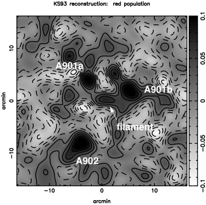
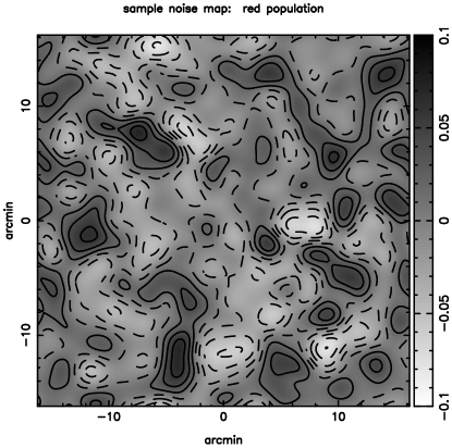
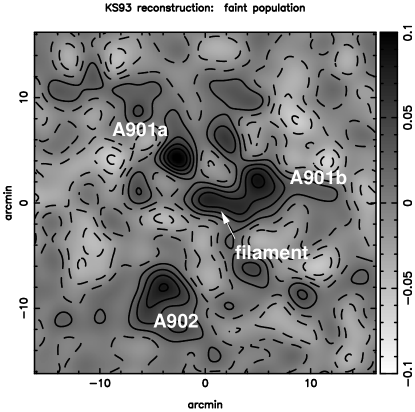
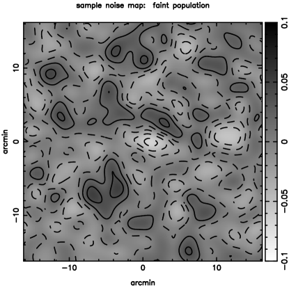
Figure 12: Non-parametric mass reconstructions and noise levels. Left: Dimensionless surface mass density, $\kappa_{M}$, reconstructions applying the Kaiser & Squires (1993) algorithm to the ‘red’ (top) and ‘faint’ (bottom) background populations (not independent). All three clusters appear as prominent mass peaks, and there is evidence in both maps of possible filamentary structure between A901b and A901a. Right: Demonstration of the noise levels for each mass map, created by randomly shuffling the ellipticities of the background galaxies but maintaining the same positions prior to the reconstruction. All reconstructions are smoothed with a $\sigma=60$ arcsec Gaussian.

It is immediately apparent from examining the mass reconstructions obtained from the ‘red’ and ‘faint’ samples of background galaxies (shown in Fig. 12) that the mass peaks corresponding to the three clusters are each strongly detected and are fairly regular in appearance. The magnitude of the mass concentrations follows the same ordering according to mass as inferred from the strength of the tangential shear profiles (from lowest to highest mass: A901a, A901b, A902). In addition, there is evidence of filamentary structure connecting A901a and A901b. We shall return to this in more detail in §5.4.

To gain an estimate of the noise levels associated with these mass reconstructions, we randomly shuffled the ellipticities of the background galaxies while maintaining their positions, and performed the mass reconstruction for each of 32 realizations of the background galaxies. Sample noise maps for the two reconstructions are shown in the right panels of Fig. 12. These levels are in agreement with the variance predicted from the KS93 algorithm, given the smoothing scale $\theta$ and mean surface density $\bar{n}$:

$$\langle\kappa^{2}\rangle=\frac{\langle\gamma^{2}\rangle}{8\pi\bar{n}\theta^{2}}.$$ (20)

Assuming a value of $\langle\gamma^{2}\rangle\simeq 0.2$ for the variance due to the intrinsic shapes of galaxies, equation (20) predicts $1\sigma$ uncertainty in $\kappa$ of 0.019 for the ‘red’ mass map and 0.014 for the ‘faint’ mass map.

The reconstruction obtained from the ‘blue’ sample of galaxies is markedly different from the red reconstruction, however. In the blue map (not shown), the cluster peaks are not present or are offset from their positions in the red map. In addition, there is an additional prominent mass peak west of A902 that does not appear in the red map, nor does it appear to be associated with any concentration of bright foreground galaxies. The dilution of the lensing signal from the clusters is not entirely surprising, given that by selecting galaxies with $B-R$ colors bluer than the supercluster galaxies one would expect to select mostly foreground galaxies or blue cluster members.

Furthermore, progressive slices in $R$-band magnitude of the blue catalogue reveal that the new mass peak is due to the ellipticities of only the faintest $(R>26)$ galaxies, for which the shape measurements are least reliable. We therefore conclude that the peak in the mass map derived from the ‘blue’ sample is likely to be spurious and the result of noise. In fact, this confirms that most of the lensing signal seen in the faint mass reconstruction is contained in the redder galaxies, and that the noise estimate for the faint reconstruction has been somewhat underestimated as the actual number density $n$ of galaxies contributing to the lensing signal is less than quoted in Table 5.3.

5.4 Detection of a dark matter filament

The mass reconstructions of Fig. 12 show evidence of an extension of the mass distribution of A901b in the direction of A901a. This is supported by the presence of an elongation of the distribution of galaxies in that region (Fig. 9). However, we note that the most prominent part of this mass ‘filament’ extends in the east-west direction and is located almost in the center of our image. This is very close to the intersection of the corners of four of the subregions on which we performed the PSF correction and so is worthy of reexamination. While we saw no sharp discontinuities in the behavior of the PSF at this location, the stars used for the corrections do only finitely sample the PSF on the chip and the bicubic polynomials could fail to properly correct this region if the anisotropies were large and varying.

To test the robustness of the PSF correction and the recovery of the filament in the mass maps, we first redid the PSF correction by fitting a seventh-order two-dimensional polynomial across the entire field (rather than applying our previous method of applying a lower-order correction separately to each subregion). However, this higher-order polynomial correction still left the largest residuals in the corrected stellar ellipticities in the central regions of the image.

Since shear is a non-local measurement, and considering that the catalogue of background galaxies already contains a small number of regions masked out due to contamination by bright stars, we then tested the effect of removing several regions of the catalogue in which the ellipticity measurements might be less reliable. Excising the central $2\arcmin\times 2\arcmin$ from the catalogue of background galaxies, we again performed the mass reconstructions. We found that the peak of the filamentary structure fell by $\Delta\kappa\simeq 0.02$ but that the underlying plateau connecting A901a and A901b was still present at the $\kappa\simeq 0.04-0.06$ levels (i.e., $\sim 2-3\sigma$ above the noise). While having holes in the input catalogues is not ideal for the purposes of the mass reconstruction, this gives some indication that at least some of the signal is real and significant. Similar results were found when we removed not only the central regions but also masked out the intersections of the regions used in the PSF correction and the regions in the corners of the image. These are regions in which any departures from the linear astrometric corrections of §2.3 could cause objects to be misaligned and would lead to a smearing of their shapes in the final combined image, which could then be misinterpreted as a lensing induced shear. However, even after such conservative cuts to the object catalogue, the filamentary structure connecting A901a and A901b continued to be detected in the mass reconstructions at a level significantly above the noise.

As an additional test, we attempted to perform the mass-reconstructions on object shape parameters derived from the $B$-band image, to check if the filament appeared in reconstructions in both bands. However, the less favorable atmospheric conditions and shorter exposure time for this image meant that we were unable to measure reliable $B$-band shapes for a sufficient number of galaxies to create a mass map.

The fact that the observed filament does not lie directly along the axis connecting the structure, but instead arcs from one to the next could be reflective of the initial orientation of the clusters. Bond et al. (1996) demonstrate how the tidal gravitational field at location of initial density peaks can create filaments with a variety of orientations and density contrasts, including the qualitative shape observed here. Given that matter filaments have long been a robust prediction of the dark matter scenario, regardless of the nature of the dark matter, this detection provides good confirmation of their existence, and hence generally supports the dark matter scenario.

6 Comparing mass and light

Comparison of the mass reconstructions with the smoothed surface number density and luminosity maps presented in Fig. 13 reveals two different descriptions of the supercluster. Contrary to the mass maps, in both light and number density the most prominent of the three clusters is by far A901a. Furthermore, the optical appearance of A901b is much more elongated and much less regular than the mass reconstructions (and the compact nature of the X-ray emission from this cluster) would suggest.

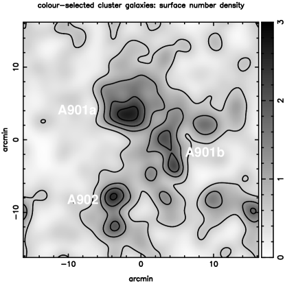
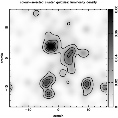
Figure 13: Smoothed distributions of supercluster galaxy density and luminosity. Left: Surface number density of the bright ($R<20$) color-selected cluster galaxies (arcmin^-2), smoothed with a $\sigma=60$ arcsec Gaussian. Right: Luminosity-weighted distribution of the same galaxies, showing the prominence of the A901a light distribution.

6.1 $M/L$ ratios in apertures

We estimate actual $M/L$ ratios for each cluster by computing the ratio of the total mass inferred from the two-dimensional reconstructions with the total $B$-band luminosity of the color-selected early-type galaxies within an aperture. Note that the mass is subject to a possible upward correction due to the insensitivity of the weak shear method to a uniform mass distribution along the line of sight (the ‘mass-sheet degeneracy’), so formally our mass estimates, and hence $M/L$ ratios, are lower limits. However, the field of view of our image is sufficiently large (and the clusters themselves are well-removed from the edges) that we may assume that $\kappa\rightarrow 0$ at the edge of the reconstructions.

The $M/L$ values listed in Table 5.2.1 show that the clusters display a range of $M/L$ ratios. We find that the $M/L$ ratios for A901a are significantly lower for all aperture sizes than the values for A901b and A902, which are in much better agreement with each other. We note, however, that the $M/L_{B}$ ratios quoted here consider the total mass, but only the contribution of the early-type galaxies to the luminosity. The large fraction of bright blue galaxies seen in Abell 902 could serve to increase the total luminosity of the cluster and thus lower the $M/L$ ratio for that cluster. The discrepancies between the values for all three clusters would, however, still remain.

Figure 14: $M/L$ ratios with increasing aperture size for each of the three clusters (points for A902 have been slightly shifted horizontally for clarity). There is no strong evidence for a change in $M/L$ ratio with scale for any of the clusters, except for the spike at $r=2$ arcmin for A901b which reflects the misalignment of mass and light in this cluster. A901a shows a significantly lower $M/L$ ratio than the other clusters for all aperture sizes. The apertures for A901a and A901b begin to overlap at $r=3.9$ arcmin.

Fig. 14 shows the resulting $M/L$ ratios for each cluster as the aperture size is varied. There is no evidence for an increase of $M/L$ ratio with aperture size for any of the clusters beyond 2 arcmin ($0.2h^{-1}$ Mpc), implying that there is no appreciable reservoir of dark matter in the inter-cluster regions. The values appear to converge at $M/L\sim 200h$ at large radii, albeit with some overlap between apertures. The dark matter distribution appears no more extended than the distribution of early-type galaxies (although as we have seen previously in the case of A901b, the two are not always precisely co-located).

6.2 Predicting mass from light

So that we may further compare mass and light across the whole field of view, we next create a prediction of the surface mass density, $\kappa_{L}$, from the luminosity of the color-selected supercluster galaxies. We determine the $k$-correction appropriate for early-type galaxies at $z=0.16$ using the population synthesis models of Bruzual & Charlot (1996) for a passively evolving early-type galaxy formed with a single burst of star formation at $z=5$. We convert observed $B$-band magnitude into luminosity, $L_{B}$, for each foreground galaxy. We can then calculate the the contribution of each galaxy to the surface mass density in a region by $mass\ density=light\times(M/L)/area$. Dividing by the critical surface mass density we find the dimensionless surface mass density

$$\kappa_{L}d\Omega=\frac{L_{B}M/L}{D_{d}^{2}}\frac{1}{\Sigma_{\rm crit}}=\frac{L_{B}300h\Upsilon M_{\odot}/L_{\odot}}{D_{d}^{2}\Sigma_{\rm crit}}.$$ (21)

As a first estimate, we assume a constant $M/L_{B}=300h$, $\Upsilon=1$ to create the predicted $\kappa_{L}$ map. This will be revised later by varying the normalization $\Upsilon$. We choose to predict the mass from the observed light, rather than the other way round, because formally the uncertainties are less: we can observe the positions and luminosities of the galaxies to create the light map.

The resulting $\kappa_{L}$ differs from the mass map recovered from our weak shear analysis in that it is non-negative everywhere with different noise properties. So that we are able to directly compare $\kappa_{L}$ and $\kappa_{M}$, we follow the procedure of Kaiser et al. (1998) and Wilson, Kaiser, & Luppino (2001, hereafter WLK). Using the estimate for $\kappa_{L}$ constructed as described in equation (21) but smoothed on a finer scale, we solve the two-dimensional Poisson equation to recover the projected lensing potential. We then derive a shear field from this potential and sample the field at the location of our background galaxy catalogue to emulate the finite sampling of our observations.

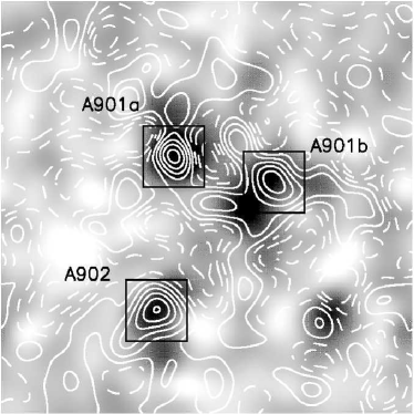
Figure 15: Comparison of surface mass density $\kappa$ predicted from the luminosity of early-type galaxies ($\kappa_{L}$, gray-scale) and that recovered from the weak shear reconstructions ($\kappa_{M}$, contours). The light from the early-type galaxies generally traces the mass, except in the case of A901b. Note that the clump of supercluster galaxies west of A902 (see Fig. 9 shows up as a prominent fourth peak in the $\kappa_{L}$ map. The mass contours show a slight overdensity in $\kappa_{M}$ near this location, but not necessarily one that would be identified as a structure from the lensing signal alone.

At this point the predicted shear field is still idealized, as it does not contain the noise associated with the intrinsic ellipticity of the background sources. To each value sampled from the shear field, we therefore add a random noise component drawn from a Gaussian distribution with $\sigma=0.3$, which reflects the measured noise from our galaxy catalogue. We then apply the KS93 algorithm to the predicted catalogue, to produce a new $\kappa_{L}$ with the same finite-field effects and similar noise properties as our measured $\kappa_{M}$ (although still insensitive to any structure outside the field of view).

The resulting predicted surface mass density, $\kappa_{L}$, and that recovered from the weak shear reconstructions, $\kappa_{M}$, are overlayed in Fig. 15. The light from the early type galaxies traces the location of the mass fairly well, with the notable exception of the elongated optical appearance of A901b, which is also displaced from the associated strongly detected mass peak. A fourth peak is predicted in the $\kappa_{L}$ map at the location of the subclump of supercluster galaxies west of A902 (see Fig. 9, right), and this is marginally reproduced in the $\kappa_{M}$ map.

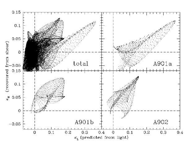
Figure 16: Pixel-by-pixel comparison of observed $\kappa_{M}$ and predicted $\kappa_{L}$ maps. The top left panel represents the entire field of view, while the remaining panels display pixels within the boxes around each of the clusters shown in Fig. 15. Note that the misalignment of light and mass in A901b produces a much broader distribution of points than the more linear relations for A901a and A902.

A pixel-by-pixel comparison of the two $\kappa$ maps is shown in Fig. 16. Additionally, the scatterplots for the regions centered around each mass peak (indicated by the boxes in Fig. 15) are shown separately for clarity. The broad distribution of the A901b points relative to the other two illustrates the general misalignment between light and mass in this cluster. Conversely, the close alignment between mass and light for the remaining two clusters is reflected in the much narrower relation. The slope of the linear relation in each case reflects the degree to which the $M/L$ ratio assumed for the predicted $\kappa_{L}$ map approximates the true value for that cluster. The differing slopes for A901a and A902 confirms that a single $M/L$ does not satisfy both clusters.

6.3 Cross-correlation of mass and light

6.3.1 Global cross-correlations

While in §6.1 and §6.2 we investigated the local properties of the mass and light, it is also useful to study the global properties of the field. In this section, we will perform a statistical cross-correlation and auto-correlations of the predicted $\kappa_{L}$ and measured $\kappa_{M}$ mass maps. We shall assume a simple linear biasing model, in which the light is related to the mass by a constant, scale-independent $M/L$ ratio. We recognize that this is unlikely to be the optimal model given the scatter in the cluster $M/L$ ratios (cf. Fig. 14). However, such a model will serve as a relatively simple starting point for this analysis and has the added advantage of allowing us to compare results with those of Kaiser et al. (1998). We write

$$\kappa_{L}=\Upsilon^{-1}\kappa_{M}+\epsilon,$$ (22)

where $\epsilon$ is a stochastic component (Dekel & Lahav, 1999) with variance $\sigma_{\epsilon}^{2}$, and $\Upsilon$ is the normalization required to correct the assumed $M/L=300h$ of equation (21) to the true $M/L$ ratio. The stochastic component, $\epsilon$, reflects the hidden variables due to all the nonlinear, nonlocal influences on galaxy and star formation not directly associated with the local density field. Note that $\langle\epsilon\rangle=0$. Later we will discuss the possibility that $\Upsilon$ is some more complicated function of scale or mass, but for the following analysis make the assumption of Kaiser et al. (1998) that a single, constant, scale-independent $M/L$ ratio can describe the whole supercluster region.

Although there are physical arguments for starting with mass and attempting to discover a relation that allows one to recover the light, for practical reasons we shall follow the opposite route and consider

$$\kappa_{M}=\Upsilon(\kappa_{L}-\epsilon).$$ (23)

As discussed earlier, this is motivated by the fact that our measurement of the mass is relatively noisy compared to the light.

We define the two-dimensional cross-correlation of two images $A$ and $B$ as

$$C^{AB}({\delta\theta})=\langle\kappa_{A}({\theta})\kappa_{B}({\theta+\delta\theta})\rangle$$ (24)

where we average over the products of all pairs of pixels separated by $\delta\theta$.

Using the linear biasing model of equation (23), the cross-correlation of $\kappa_{M}$ and $\kappa_{L}$ becomes

$$\begin{array}[]{rcl}C^{ML}&=&\langle\kappa_{L}\kappa_{M}\rangle\\ &=&\langle\kappa_{L}[\Upsilon(\kappa_{L}-\epsilon)]\rangle\\ &=&\Upsilon\langle\kappa_{L}^{2}\rangle,\end{array}$$ (25)

since $\epsilon$ and $\kappa_{L}$ are assumed to be uncorrelated. Similarly, the autocorrelation of $\kappa_{M}$ becomes

$$\begin{array}[]{rcl}C^{MM}&=&\langle\kappa_{M}\kappa_{M}\rangle\\ &=&\langle([\Upsilon(\kappa_{L}-\epsilon)][\Upsilon(\kappa_{L}-\epsilon)]\rangle\\ &=&\Upsilon^{2}\langle\kappa_{L}^{2}\rangle+\Upsilon^{2}\sigma_{\epsilon}^{2},\end{array}$$ (26)

and the autocorrelation of $\kappa_{L}$ is simply

$$C^{LL}=\langle\kappa_{L}^{2}\rangle.$$ (27)

We can therefore calculate all three of these relations and determine values for $\Upsilon$ and $\sigma_{\epsilon}^{2}$.

However, to obtain an unbiased estimate of these correlation functions, we need to remove the noise, as in

$$C^{LL}_{\rm true} = C^{LL}_{\rm obs}-C^{LL}_{\rm noise},$$ (28)

$$C^{MM}_{\rm true} = C^{MM}_{\rm obs}-C^{MM}_{\rm noise},$$ (29)

$$C^{ML}_{\rm true} = C^{ML}_{\rm obs}.$$ (30)

Note that the noise properties of $\kappa_{L}$ and $\kappa_{M}$ are uncorrelated.

We estimate $C^{MM}_{\rm noise}$ by constructing an ensemble of 32 mass maps from randomized versions of our faint galaxy catalogues in the same manner and with the same smoothing scale as $\kappa_{M}$. For each realization, the positions of the background galaxies remain fixed while the ellipticities of the galaxies are shuffled, and these noise maps (e.g. the right-hand panels of Fig. 12) are used to calculate the average autocorrelation of the noise, $C^{MM}_{\rm noise}$. We calculate $C^{LL}_{\rm noise}$ in a similar way by randomizing our catalogue of predicted shear values.

Figure 17: The radial dependence of the two-dimensional cross-correlation of mass and light, $C^{ML}$ (top left) and the auto-correlations $C^{MM}$ (top right) and $C^{LL}$ (bottom left). In each case, the solid curves show $C^{LL}$ renormalized according to equations (25)–(27) and the best-fit values of $\Upsilon=0.422$ and $\sigma_{\epsilon}^{2}=0$. The assumption of a linear bias model breaks down on the scales of the average cluster separation, $r\sim 10$ arcmin, reflecting the significantly different $M/L$ ratios for the individual clusters. Note that the points are not independent. The bottom right panel shows the sampled points from all three curves used in the $\chi^{2}$ analysis, renormalized to agree with $C^{LL}$.

Fig. 17 shows the azimuthally averaged $C^{LL}_{\rm true}$, $C^{ML}_{\rm true}$, and $C^{MM}_{\rm true}$ curves, with error bars calculated from the noise reconstructions. Note the significance of the correlation signal at small scales in each case: e.g. for $C^{ML}$, the zero-lag correlation between mass and light is significant at the 10.6$\sigma$ level. On larger scales, the mass auto-correlation, $C^{MM}$, displays oscillations not present in the other two curves.

To recover values for $\Upsilon$ and $\sigma_{\epsilon}$, we proceed with a $\chi^{2}$ test on equations (25)–(27). The points on the correlation functions are highly correlated, so we sample the curves at 60 arcsec intervals (the Gaussian smoothing width) to approximate independence. The parameters producing the minimum $\chi^{2}$ value are $\Upsilon=0.442$ and $\sigma_{\epsilon}^{2}=0$, i.e. a $M/L_{B}=126h$ and no detection of a non-zero stochastic component. The $\chi^{2}$ distribution is shown in Fig. 18. For comparison, $C^{LL}$ is renormalized according to equations (25)–(27) using the fitted values for $\Upsilon$ and $\sigma_{\epsilon}$, and the resulting curves are shown by the solid line in each of the first three panels of Fig. 17. The lower right panel of Fig. 17 shows the sampled points used in the $\chi^{2}$ analysis, renormalized to agree with $C^{LL}$.

At zero-lag the agreement between the three curves is not particularly good, and the amplitudes of the curves at $r=0$ imply $M/L\sim 150h$. Neither the $\chi^{2}$ nor the zero-lag value for the $M/L$ ratio is in good agreement with the much higher $M/L$ ratios tabulated for A901b and A902 in Table 2.1. Furthermore, the minimum value of the $\chi^{2}$ function for the 17 sampled points is 34, indicating that the linear bias model is not a good choice. The model breaks down to a greater degree on larger scales. In particular, the $\kappa_{M}$ autocorrelation function $C^{MM}$ shows a prominent secondary bump at $r\sim 11$ arcmin ($\sim$ 1 Mpc) that is missing from $C^{MM}$ and $C^{LL}$. This scale length roughly corresponds to the average separation of the clusters and reflects the variation in luminosity (and $M/L$ ratios) between the clusters. While the peaks are of similar size in the mass map $\kappa_{M}$ (producing the secondary peak in $C^{MM}$ at $r\sim 11$ arcmin), the peaks in the mass-from-light map $\kappa_{L}$ vary in amplitude, most notably for the relatively underluminous A901b. Thus the assumption of a linear biasing model with a single $M/L$ ratio describing the entire supercluster fails on these scales. Nevertheless, Fig. 17 shows that the light from the early-type galaxies and the surface mass density agree surprisingly well within the errors.

Figure 18: Results of $\chi^{2}$ fit for parameters $\Upsilon$ and $\sigma_{\epsilon}^{2}$ in equations (25)–(27). The best-fit parameters are $\Upsilon=0.442$ and $\sigma_{\epsilon}^{2}=0$, corresponding to $M/L_{B}=126h$ and providing no evidence for a stochastic bias component. The contours show $\Delta\chi^{2}=2.3,6.17$ which enclose the 68% and 95% confidence limits for a two-parameter fit. Inset: the $\chi^{2}$ contours for a Gaussian model for the stochastic component, $\sigma_{\epsilon}^{2}\rightarrow\sigma_{\epsilon}^{2}A(r)$, where $A(r)=\exp[\frac{-(r-r^{\prime})^{2}}{2r_{s}^{2}}]/\sqrt{2\pi r_{s}^{2}}$, and $r_{s}$ is the smoothing scale (1 arcmin). The best-fit value shown corresponds to the zero-lag value $\sigma_{\epsilon}^{2}A(0)=5.97\times 10^{-4}$, with the resulting $M/L$ ratio unchanged.

In response to the poor agreement of the correlation function on small scales, we consider an additional model for the stochastic component: a $\delta$-function at zero-lag that is modified by a Gaussian function representing the smoothing scale of the light and mass maps. A non-zero measurement of a stochastic term will therefore likely be a measure of the scatter in the $M/L$ ratio of the clusters themselves. In this case, the autocorrelation of the stochastic component at separation $r-r^{\prime}$ is

$$\langle\epsilon(r)\epsilon(r^{\prime})\rangle=\sigma_{\epsilon}^{2}\delta_{k}(r-r^{\prime}),$$ (31)

and so

$$\sigma_{\epsilon}^{2}\rightarrow\sigma_{\epsilon}^{2}\frac{\exp\left[{\frac{-(r-r^{\prime})}{2r_{s}^{2}}}\right]}{\sqrt{2\pi r_{s}^{2}}},$$ (32)

where $r_{s}=1$ arcmin is the smoothing scale for our analysis. Using this model, the results of the $\chi^{2}$ are shown in the inner panel of Fig. 18. We find a non-zero value for the stochastic component at zero-lag and an unchanged $M/L$ ratio. However, the minimum value of the $\chi^{2}$ function (31 for 17 data points) demonstrates that the fit is only marginally improved, and so the detection is tentative at best. A more sophisticated model (with, for example, a varying $M/L$ ratio) would be more likely to improve the fit.

6.3.2 Cross-correlation of individual clusters

To further explore the degree of correlation between light and mass on the scales of the individual clusters, we perform cross-correlations of $\kappa_{L}$ and $\kappa_{M}$ on pixels extracted from boxes around each of the three clusters (shown in Fig. 15). As in this case we are concerned not with the normalization of $\kappa_{L}$ but with the spatial alignment between the two distributions, we use a cross-correlation estimator normalized by the variances of the overlapping pixels at each image offset. The resulting two-dimensional cross-correlations are shown in Fig. 19 for the entire field and for the three clusters. The misalignment of light and mass in A901b is especially apparent, while A902 also shows an elongated mass distribution with respect to the light.

The correlation coefficient, $C$, can be written as

$$C=\frac{\langle\kappa_{M}\kappa_{L}\rangle}{\sqrt{\langle\kappa_{M}^{2}\rangle\langle\kappa_{L}^{2}\rangle}}=\frac{1}{\sqrt{1+\sigma_{\epsilon}^{2}/\langle\kappa_{L}^{2}\rangle}}.$$ (33)

For Fig. 17, the zero-lag values give $C=0.916$, or $\sigma_{\epsilon}=0.04\langle\kappa_{L}^{2}\rangle^{1/2}\simeq 5.3\times 10^{-4}$, while for Fig. 19 we find $C=0.44$ for the entire field. This apparent inconsistency could be due to the fact that for the cross-correlations of Fig. 19 the contribution from to the noise was not removed (cf. eqs. [28]–[30]), reducing the magnitude of the correlation.

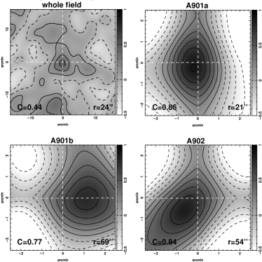
Figure 19: Two-dimensional cross-correlation of the $\kappa_{L}$ and $\kappa_{M}$ for the whole field (top left) and for pixels extracted from the boxes around each of the three clusters in Fig. 15. The misalignment of light and mass in A901b is especially evident, as is the elongation of the mass distribution in A902 with respect to the light. Values of $C$ and $r$ give the magnitude and offset of the peak of the correlation function in each case.

7 Discussion and conclusions

One of the most striking aspects of the A901/902 supercluster is how it reveals itself in many different guises according to the observations at hand. Were one to take the revised X-ray luminosities of Schindler (2000) at face value, it would appear that only one moderate X-ray cluster is to be found in this region, at the location of A901b. When one examines the number density of color-selected galaxies (Fig. 13, left), however, the picture becomes more complex. One would conclude (e.g. Abell et al., 1989) that there are in fact two clusters in the field (A901a and A902 in our nomenclature). A third overdensity near the location of A901b could be considered, but it appears not nearly as prominent as the other two.

Weighting the number density of early-type galaxies by luminosity (Fig. 13, right) changes the picture still further. Now it is A901a that leaps to prominence, dwarfing the other two clusters with a compact collection of bright early-type galaxies. However, factoring the fraction of blue galaxies missed by the color-selection could boost the total luminosity of A902 due to the relatively large population of bright blue galaxies in its vicinity.

How does one make sense of these conflicting portraits of the supercluster? In this case, gravitational lensing provides a direct link to the underlying mass distribution, and hence to theoretical predictions of structure formation. It also provides an additional complication, as in the mass map (Fig. 12) one now sees three strongly detected mass peaks. The relative strength of each of the lenses (Fig. 11) is contrary to the number density, light, or X-ray predictions, with A902 appearing the most massive and A901a the least. Furthermore, the mass distribution of A901b is significantly misaligned with the early-type light (Fig.15).

We used a statistical cross-correlation to examine the relationship between the early-type galaxy light distribution and the underlying dark matter. The light and mass are strongly correlated at the 10.6$\sigma$ level at zero lag. Despite the fact that the clusters exhibit a range of $M/L$ ratios (total mass to early-type light), we find that the simple linear biasing model yields somewhat good agreement between the cross- and auto-correlations of mass and light, and do not find evidence for a stochastic component. The best-fit parameters imply that the mass is well traced by the light from the early-type galaxies with $M/L_{B}=126h$, which is an underestimate compared with the average $M/L\sim 200h$ computed locally for the clusters themselves. This could reflect that there is more light than mass extended throughout the field, but is more likely due to the fact that on large angular scales (on the order of the separation between the clusters) and on small scales, the relation breaks down and the linear biasing model itself is not an adequate description.

While the $M/L$ ratios of the clusters do not increase at large scales (Fig. 14), a single $M/L$ ratio is not an appropriate description, despite their proximity to one another. There are a number of possible ways to reconcile these differences. The first option is to attribute it simply to a difference in the mix of galaxy populations in the various clusters. For example, we could modify the observed $M/L$ ratios (which consider only the luminosity of the color-selected early-type galaxies) by including the contribution of the late-types galaxies. This would require an estimate of spectral or morphological type and a confirmation of supercluster membership via redshift information, all of which will possible with the forthcoming photometric redshifts soon to be available for this system. In this way, we could develop a more complete picture of the galaxy populations for each cluster, and test if the mass-light correlation for spirals is more extended than the strong correlation between mass and ellipticals we detect here. As we have seen in §4.2, the galaxy populations also appear to vary from cluster to cluster. The potential large blue fraction of galaxies around A902, if attributed to late-type luminous cluster members, could boost the luminosity of the cluster and bring its $M/L$ ratio more in line with that of A901a. However, this would still leave the anomalous case of A901b, with its high $M/L$ ratio and misaligned distributions of mass and light.

A second possible explanation for the non-uniformity of the system could be the effects of on-going mergers and interactions between the clusters, which are in close proximity to one another (the average separation being $\sim$1 Mpc). We have seen in the mass map that a filament of dark matter may connect A901a and A901b, and is mostly unassociated with light from the early-type galaxies. However, Fig. 9a shows that some bright galaxies do lie in that region and were too blue to survive the early-type color selection. In this case, a spectroscopic survey of bright galaxies of the field could look for signs of enhanced star formation in this region. Perhaps the extra luminosity of A901a relative to the other two clusters, or the presence of bright blue galaxies along the filament, is attributable to enhanced star formation triggered by cluster infall or cluster-cluster interactions. This would bias the $M/L$ ratio of A901a low relative to the other two clusters.

Finally, some form of non-linear biasing may be required to relate the light and mass, with the $M/L$ ratio being some more complicated function of the local density field. We note that for our supercluster, the most massive clusters have the higher $M/L$ ratios, and the least massive cluster has the smallest $M/L$ ratio for all aperture sizes, implying a mass-dependent scaling relation between mass and light. This highlights the importance of having a comprehensive mass-selected sample of galaxy clusters to test the dependence of the $M/L$ and other properties on cluster mass.

Kaiser et al. (1998) presented the first weak lensing study of a supercluster, in that case a system of three massive X-ray clusters at $z=0.42$. Our study complements this by examining a similar system, but one that is less massive, at lower redshift, and more compact. Our results differ in that we do not see nearly as strong agreement between $C^{LL}$ and $C^{ML}$ as in their study (e.g. their Fig. 20). We note, however, that our approach differs by removing the contribution of noise from the correlation function (cf. eqs. [28]–[30]). They also do not include the mass auto-correlation function, $C^{MM}$, in their analysis, which in the case of the data presented here (see Fig. 17), displays significant oscillatory structure that challenges the linear biasing model. It remains to be seen if their single $M/L$ ratio would simultaneously satisfy all three correlation functions: $C^{LL},C^{ML}$ and $C^{MM}$.

One of the most striking implications of the Kaiser et al. (1998) results was the low value of $\Omega_{m}$ determined under the assumption that their measured $M/L=280h$ is universal. Assuming that early-types contribute 20% of the total luminosity density of the Universe, they find $\Omega\simeq 0.04$ for a Universe with critical $(M/L)_{\rm crit}=1500h$. This would imply an extremely low density Universe, with no need to invoke large amounts of non-baryonic dark matter. A follow-up study by WLK attempted to further investigate these findings with an identical weak lensing and cross-correlation analysis. The targets in this case were six blank fields, chosen to be free of any known structures and thus potentially more representative of the universal $M/L$ ratio than dense environments that may be biased or display complicated environmental effects. Following a similar analysis, they found $M/L_{B}\simeq 300\pm 75h$ for a flat ($\Omega_{m}=0.3,\Omega_{\Lambda}=0.7$) cosmology, and $M/L_{B}\simeq 400\pm 100h$ for Einstein-de Sitter, consistent with the Kaiser et al. results.

Rather than estimating the fractional contribution of the early-types to the luminosity density of the Universe, WKL directly integrated over the type-dependent luminosity function from the 2dF redshift survey (Folkes et al., 1999). For $M/L_{E}=300h$, this yields $\Omega\simeq 0.1\pm 0.02$ ($\Omega\simeq 0.13\pm 0.03$ for the WLK results in an Einstein-de Sitter Universe). These are higher than the Kaiser et al. (1998) supercluster results and do require some component of exotic matter to contribute to the total mass density. However, we note that were we to apply the same, more rigorous calculation to the Kaiser et al. $M/L=280h$, this would yield $\Omega_{m}=0.09$, more than twice their original estimate.

In summary, both the Kaiser et al. (1998) and WKL studies find that most of the mass in the Universe is associated with early-type galaxies, and in the case of the Kaiser et al. (1998) supercluster the mass is no more extended than the distribution of the early-types. The low values of $\Omega_{m}$ obtained in this fashion assume that little mass is associated with late-type galaxies (under the assumption that an extended distribution of massive spiral galaxies is not reflected in the concentrated distributions of mass), and so assigned a negligible $M/L$ ratio to the late-types. This assumption is supported by the findings of Bahcall et al. (1995) who find ellipticals to have four times the mass of spirals for the same luminosity. Our conclusions are roughly similar but with some important differences. Firstly, we do not see nearly the same agreement between mass and light in our supercluster relative to the Kaiser et al. (1998) study, both in the spatial distributions (e.g. A901b, Fig. 19) and in the $M/L$ ratios (Fig. 14). Secondly, the global $M/L$ ratio (considering the total mass and the early-type light) that we determine from the $\chi^{2}$ fit to the cross- and auto-correlations functions is lower, $M/L_{B}\simeq 130h$, which, following the same arguments as above, would yield $\Omega_{m}=0.04$. However, this rests on the assumption that the linear bias model is correct and that the global $M/L$ ratio we measure is representative. The failure of the correlation functions to agree in shape and amplitude on small and large scales shows that this assumption is not valid.

The clusters in the supercluster presented here are clearly not isolated nor relaxed systems. The effects of a pre- or post-major merger state could be invoked to explain the discrepancies between the alignment of mass and light. In both distributions, evidence for inter-cluster material is seen in the form of filamentary structures between A901a and A901b, and some degree of non-linear biasing is likely.

A wealth of additional information about this system is available in the form of the photometric redshifts, which will be derived from the remaining 15 filters in which this field was observed. Aside from allowing an independent measurement of the mass distribution by measuring the effects of the gravitational magnification on the luminosity function of the background galaxies, the redshifts will allow for a more accurate characterisation of the foreground structure than the relatively crude color-cuts employed here. Furthermore, rather than concentrate solely on the color-selected early-type galaxies, a more comprehensive picture of the mass-light relation will be constructed by separating structures in redshift space and by spectral class. This could include compensating for the effects of foreground or background structures along the line of sight to disentangle projection effects that could bias the two-dimensional weak lensing mass measurements. Additionally, one could perform correlations between mass and spectral type to determine how much mass is in fact associated with the late-type galaxies. Finally, a spectroscopic survey of the bright galaxies in this region could provide the final piece of the puzzle, by providing dynamical information and tracing star formation as a function of environment (i.e. in the filament or infall regions).

References

- Abell (1958) Abell, G. O. 1958, ApJS, 3, 211
- Abell et al. (1989) Abell, G. O., Corwin, H. G., & Olowin, R. P. 1989, ApJS, 70, 1
- Baade et al. (1998) Baade, D., et al., 1998, The Messenger, 93, 13
- Baade et al. (1999) Baade, D., et al., 1999, The Messenger, 95, 15
- Baade (1999) Baade, D., 1999, ESO WFI User Manual, Doc. No. LSO-MAN-ESO-22100-00001
- Bacon et al. (2000) Bacon, D. J., Refregier, A. R., & Ellis, R. S. 2000, MNRAS, 318, 625
- Bahcall et al. (2000) Bahcall, N. A., Cen, R., Davé, R., Ostriker, J. P., & Yu, Q. 2000, ApJ, 541, 1
- Bahcall et al. (1995) Bahcall, N. A., Lubin, L. M., & Dorman, V. 1995, ApJ, 447, L81
- Bartelmann & Schneider (2001) Bartelmann, M. & Schneider, P. 2001, Physics Reports, 340, 291
- Bertin & Arnouts (1996) Bertin, E. & Arnouts, S. 1996, A&AS, 117, 393
- Bond et al. (1996) Bond, R., Kofman, L., & Pogosyan, D. 1996, Nature, 380, 603
- Briel & Henry (1995) Briel, U. G. & Henry, J. P. 1995, A&A, 302, L9
- Bruzual & Charlot (1996) Bruzual, G. & Charlot S., 1996, Documentation for gissel96 Spectral Synthesis Code
- Carlberg et al. (1996) Carlberg, R. G., Yee, H. K. C., Ellingson, E., Abraham, R., Gravel, P., Morris, S., & Pritchet, C. J. 1996, ApJ, 462, 32
- Cen et al. (1995) Cen, R., Kang, H., Ostriker, J. P., & Ryu, D. 1995, ApJ, 451, 436
- Clowe et al. (2000) Clowe, D., Luppino, G. A., Kaiser, N., & Gioia, I. M. 2000, ApJ, 539, 540
- Cohen et al. (2000) Cohen, J. G., Hogg, D. W., Blandford, R., Cowie, L. L., Hu, E., Songaila, A., Shopbell, P., & Richberg, K. 2000, ApJ, 538, 29
- Colberg et al. (1999) Colberg, J. M., White, S. D. M., Jenkins, A., & Pearce, F. R. 1999, MNRAS, 308, 593
- Condon et al. (1998) Condon, J. J., Cotton, W. D., Greisen, E. W., Yin, Q. F., Perley, R. A., Taylor, G. B., & Broderick, J. J. 1998, AJ, 115, 1693
- Dekel & Lahav (1999) Dekel, A. & Lahav, O. 1999, ApJ, 520, 24
- Ebeling et al. (1996) Ebeling, H., Voges, W., Bohringer, H., Edge, A. C., Huchra, J. P., & Briel, U. G. 1996, MNRAS, 281, 799
- Fahlman et al. (1994) Fahlman, G., Kaiser, N., Squires, G., & Woods, D. 1994, ApJ, 437, 56
- Folkes et al. (1999) Folkes, S., Ronen, S., Price, I., & et al. 1999, MNRAS, 308, 459
- Girardi et al. (1996) Girardi, M., Fadda, D., Giuricin, G., Mardirossian, F., Mezzetti, M., & Biviano, A. 1996, ApJ, 457, 61
- Hoekstra et al. (2000) Hoekstra, H., Franx, M., & Kuijken, K. 2000, ApJ, 532, 88
- Hoekstra et al. (1998) Hoekstra, H., Franx, M., Kuijken, K., & Squires, G. 1998, New Astronomy Review, 42, 137
- Kaiser & Squires (1993) Kaiser, N. & Squires, G. 1993, ApJ, 404, 441
- Kaiser et al. (1995) Kaiser, N., Squires, G., & Broadhurst, T. 1995, ApJ, 449, 460
- Kaiser et al. (2000) Kaiser, N., Wilson, G., & Luppino, G. 2000, submitted to ApJ, (astro-ph/0003338)
- Kaiser et al. (1999) Kaiser, N., Wilson, G., Luppino, G., & Dahle, I. 1999, submitted to PASP, (astro-ph/9907229)
- Kaiser et al. (1998) Kaiser, N., Wilson, G., Luppino, G., Kofman, L., Gioia, I., Metzger, M., & Dahle, I. 1998, submitted to ApJ, (astro-ph/9809268)
- Lubin et al. (2000) Lubin, L. M., Brunner, R., Metzger, M. R., Postman, M., & Oke, J. B. 2000, ApJ, 531, L5
- Luppino & Kaiser (1997) Luppino, G. A. & Kaiser, N. 1997, ApJ, 475, 20
- Maoli et al. (2001) Maoli, R., Van Waerbeke, L., Mellier, Y., Schneider, P., Jain, B., Bernardeau, F., Erben, T., & Fort, B. 2001, A&A, 368, 766
- Mellier (1999) Mellier, Y. 1999, ARA&A, 37, 127
- Moshir (1990) Moshir, M. E. A. 1990, in IRAS Faint Source Catalogue, version 2.0
- Pierre et al. (2000) Pierre, M., Bryan, G., & Gastaud, R. 2000, A&A, 356, 403
- Postman et al. (1988) Postman, M., Geller, M. J., & Huchra, J. P. 1988, AJ, 95, 267
- Quintana et al. (1995) Quintana, H., Ramirez, A., Melnick, J., Raychaudhury, S., & Slezak, E. 1995, AJ, 110, 463
- Richstone et al. (1992) Richstone, D., Loeb, A., & Turner, E. L. 1992, ApJ, 393, 477
- Schindler (2000) Schindler, S. 2000, A&AS, 142, 433
- Schlegel et al. (1998) Schlegel, D. J., Finkbeiner, D. P., & Davis, M. 1998, ApJ, 500, 525
- Small et al. (1997) Small, T. A., Sargent, W. L. W., & Hamilton, D. 1997, ApJS, 111, 1
- Van Waerbeke et al. (2000) Van Waerbeke, L., Mellier, Y., Erben, T., Cuillandre, J. C., Bernardeau, F., Maoli, R., Bertin, E., Mc Cracken, H. J., Le Fèvre, O., Fort, B., Dantel-Fort, M., Jain, B., & Schneider, P. 2000, A&A, 358, 30
- Vogeley et al. (1994) Vogeley, M. S., Park, C., Geller, M. J., Huchra, J. P., & Gott, J. R. I. 1994, ApJ, 420, 525
- Wilson et al. (2001) Wilson, G., Kaiser, N., & Luppino, G. 2001, accepted to ApJ, (astro-ph/0102396)
- Wisotzki et al. (2000) Wisotzki, L., Christlieb, N., Bade, N., Beckmann, V., Köhler, T., Vanelle, C., & Reimers, D. 2000, A&A, 358, 77
- Wittman et al. (2000) Wittman, D. M., Tyson, J. A., Kirkman, D., Dell’Antonio, I., & Bernstein, G. 2000, Nature, 405, 143
- Wolf et al. (2001) Wolf, C., Meisenheimer, K., Dye, S., Kleinheinrich, M., Rix, H.-W., & Wisotzski, L. 2001, submitted to A&A, (astro-ph/0012474)