The Mass Function of an X-Ray Flux-Limited Sample of Galaxy Clusters

Abstract

A new X-ray selected and X-ray flux-limited galaxy cluster sample is presented. Based on the ROSAT All-Sky Survey the 63 brightest clusters with galactic latitude $|b_{\rm II}|\geq 20$ deg and flux $f_{\rm X}(0.1-2.4\,{\rm keV})\geq 2\times 10^{-11}\,{\rm ergs\,s^{-1}\,cm^{-2}}$ have been compiled. Gravitational masses have been determined utilizing intracluster gas density profiles, derived mainly from ROSAT PSPC pointed observations, and gas temperatures, as published mainly from ASCA observations, assuming hydrostatic equilibrium. This sample and an extended sample of 106 galaxy clusters is used to establish the X-ray luminosity–gravitational mass relation. From the complete sample the galaxy cluster mass function is determined and used to constrain the mean cosmic matter density and the amplitude of mass fluctuations. Comparison to Press–Schechter type model mass functions in the framework of Cold Dark Matter cosmological models and a Harrison–Zeldovich initial density fluctuation spectrum yields the constraints $\Omega_{\rm m}=0.12^{+0.06}_{-0.04}$ and $\sigma_{8}=0.96^{+0.15}_{-0.12}$ (90 % c.l.). Various possible systematic uncertainties are quantified. Adding all identified systematic uncertainties to the statistical uncertainty in a worst case fashion results in an upper limit $\Omega_{\rm m}<0.31$. For comparison to previous results a relation $\sigma_{8}=0.43\,\Omega_{\rm m}^{-0.38}$ is derived. The mass function is integrated to show that the contribution of mass bound within virialized cluster regions to the total matter density is small, i.e., $\Omega_{\rm Cluster}=0.012^{+0.003}_{-0.004}$ for cluster masses larger than $6.4^{+0.7}_{-0.6}\times 10^{13}\,h_{50}^{-1}\,M_{\odot}$.

1 Introduction

The galaxy cluster mass function is the most fundamental statistic of the galaxy cluster population. It is determined by the initial conditions of the mass distribution set in the early universe in a relatively straightforward way, since the evolution of the large-scale matter distribution on scales comparable to the size of clusters and larger is linear and since the formation of clusters is governed by essentially only gravitational processes. Choosing a specific cosmological scenario provides definitive predictions about these initial conditions in a statistical sense. The overall process of the gravitational growth of the density fluctuations and the development of gravitational instabilities leading to cluster formation is comparatively easy to understand. It has been well described by analytical models (e.g., Press & Schechter 1974, Bond et al. 1991, Lacey & Cole 1993, Kitayama & Suto 1996, Schuecker et al. 2001a) and simulated in numerical gravitational $N$-body calculations (e.g., Efstathiou et al. 1988; Lacey & Cole 1994). Even though the slight deviations from the theoretical prescription found in recent simulations (e.g., Governato et al. 1999; Jenkins et al. 2001) seem to require further refinement in the theoretical framework, these deviations are too small to be significant for the current investigation, as will be shown later. For the precision needed here these large simulations therefore support the validity of the model predictions. Within this framework the observed cluster mass function provides the opportunity to test different cosmological models. The tests are particularly sensitive to the amplitude of the cosmic matter density fluctuations (at a scale of the order of 10 Mpc) as well as the normalized total matter density, $\Omega_{\rm m}$ (e.g., Henry & Arnaud 1991; Bahcall & Cen 1992).

In addition to its importance in testing cosmological models the integral of the mass function yields the interesting information on the fractional amount of matter contained in gravitationally bound large-scale structures. Using one of the first attempts to construct a mass function over the mass range from giant ellipticals to massive clusters by Bahcall & Cen (1993) Fukugita et al. (1998) obtain a mass fraction $\Omega_{\rm Group}=0.12\pm 0.02$ for $2\times 10^{12}\leq M\leq 2\times 10^{14}\,h_{50}^{-1}\,M_{\odot}$ (where the mass fraction is expressed here in units of the critical density of the universe, $\rho_{\rm c}$). This result is already close to the total matter density in some of the proposed cosmological scenarios. Therefore a precise observational determination of the integral mass function is a very important task for astronomy.

Unfortunately the galaxy cluster mass is not an easily and directly observable quantity (except for measurements of the gravitational lensing effect of clusters which may play a large role in the construction of mass functions in the future) and one has to resort to the observation of other cluster parameters from which the cluster masses can be deduced.

X-ray astronomy has provided an ideal tool to first detect and select massive clusters by measuring their X-ray luminosity and to secondly perform mass determinations on individual clusters through X-ray imaging and X-ray spectroscopy.

In this paper we report the first rigorous application of these two approaches for the construction of the cluster mass function. Building on the ROSAT All-Sky X-ray Survey (RASS) (Trümper, 1993; Voges et al., 1999), which has been well studied in the search of the brightest galaxy clusters through several survey projects (see refs in Sect. 2), we have compiled a new, highly complete sample of the X-ray brightest galaxy clusters (HIFLUGCS, the HIghest X-ray FLUx Galaxy Cluster Sample).

Thanks to the numerous detailed galaxy cluster observations performed with the ROSAT and ASCA (Tanaka et al., 1994) satellite observatories and accumulated in the archives we can perform a detailed mass determination for most of these clusters and obtain a good mass estimate for the few remaining objects. From these data we first establish a (tight) correlation of the measured X-ray luminosity and the cluster mass. This relation assures that we have essentially sampled the most massive clusters in the nearby universe, which forms the basis of the construction of the cluster mass function.

Previous local galaxy cluster mass functions have been derived by Bahcall & Cen (1993), Biviano et al. (1993), Girardi et al. (1998), and Girardi & Giuricin (2000, for galaxy groups). Bahcall & Cen (1993) used the galaxy richness to relate to cluster masses for optical observations and an X-ray temperature–mass relation to convert the temperature function given by Henry & Arnaud (1991) to a mass function. Biviano et al. (1993), Girardi et al. (1998), and Girardi & Giuricin (2000) used velocity dispersions for optically selected samples to determine the mass function. Here we use a different approach and construct the first mass function for X-ray selected galaxy clusters based on the RASS using individually determined cluster masses. The mass function of this cluster sample is then used to determine the mass fraction in bound objects with masses above a minimum mass and to derive tight constraints on cosmological scenarios.

The paper is organized as follows. In Sect. 2 the sample selection is described. The details of the determination of the observational quantities are given in Sect. 3. The results are presented in Sect. 4 and discussed in Sect. 5. The conclusions are summarized in Sect. 6.

Throughout a Hubble constant $H_{0}=50\,h_{50}\,\rm km\,s^{-1}\,Mpc^{-1}$, $h_{50}=1$, $\Omega_{\rm m}=1$, a normalized cosmological constant $\Omega_{\Lambda}\equiv\Lambda/(3\,H_{0}^{2})=0$, and a normalized curvature index $\Omega_{\rm k}\equiv 1-\Omega_{\rm m}-\Omega_{\Lambda}=0$ is used if not stated otherwise (present day quantities). We note that the determination of physical cluster parameters has a negligible dependence on $\Omega_{\rm m}$ and $\Omega_{\Lambda}$ for the small redshift range used here, as will be shown later. Therefore it is justified to determine the parameters for an Einstein–de Sitter model but to discuss the results also in the context of other models.

2 Sample

The mass function measures the cluster number density as a function of mass. Therefore any cluster fulfilling the selection criteria and not included in the sample distorts the result systematically. It is then obvious that for the construction of the mass function it is vital to use a homogeneously selected and highly complete sample of objects, and additionally the selection must be closely related to cluster mass. In this work the RASS, where one single instrument has surveyed the whole sky, has been chosen as the basis for the sample construction. Using the X-ray emission from the hot intracluster medium for cluster selection minimizes projection effects and the tight correlation between X-ray luminosity and gravitational mass convincingly demonstrates that X-ray cluster surveys have the important property of being mass selective (Sect. 4.1).

Several cluster catalogs have already been constructed from the RASS with high completeness down to low flux limits (see refs below). These we have utilized for the selection of candidates. Low thresholds have been set for selection in order not to miss any cluster due to measurement uncertainties. These candidates have been homogeneously reanalyzed, using higher quality ROSAT PSPC pointed observations whenever possible (Sect. 3). A flux limit well above the limit for candidate selection has then been applied to define the new flux-limited sample of the brightest clusters in the sky.

In detail the candidates emerged from the following input catalogs. Table 2 lists the selection criteria and the number of clusters selected from each of the catalogs, that are contained in the final sample.
1) The REFLEX (ROSAT-ESO Flux-Limited X-ray) galaxy cluster survey (Böhringer et al., 2001b) covers the southern hemisphere (declination $\delta\leq$ +2.5 deg; galactic latitude $|b_{\rm II}|\geq 20.0$ deg) with a flux limit $f_{\rm X,lim}(0.1-2.4\,{\rm keV})=3.0\,\times 10^{-12}\,{\rm ergs\,s^{-1}\,cm^{-2}}$.
2) The NORAS (Northern ROSAT All-Sky) galaxy cluster survey (Böhringer et al., 2000) contains clusters showing extended emission in the RASS in the northern hemisphere ($\delta\geq$ 0.0 deg; $|b_{\rm II}|\geq 20.0$ deg) with count rates $C_{\rm X}(0.1-2.4\,{\rm keV})\geq 0.06\,{\rm cts\,s^{-1}}$.
3) NORAS II (J. Retzlaff et al., in preparation) is the continuation of the NORAS survey project. It includes point like sources and aims for a flux limit $f_{\rm X,lim}(0.1-2.4\,{\rm keV})=2.0\,\times 10^{-12}\,{\rm ergs\,s^{-1}\,cm^{-2}}$.
4) The BCS (ROSAT Brightest Cluster Sample) (Ebeling et al., 1998) covers the northern hemisphere ($\delta\geq$ 0.0 deg; $|b_{\rm II}|\geq 20.0$ deg) with $f_{\rm X,lim}(0.1-2.4\,{\rm keV})=4.4\,\times 10^{-12}\,{\rm ergs\,s^{-1}\,cm^{-2}}$ and redshifts $z\leq 0.3$.
5) The RASS 1 Bright Sample of Clusters of Galaxies (De Grandi et al., 1999) covers the south galactic cap region in the southern hemisphere ($\delta<$ +2.5 deg; $b_{\rm II}<-20.0$ deg) with an effective flux limit $f_{\rm X,lim}(0.5-2.0\,{\rm keV})$ between $\sim$ 3 and $4\,\times 10^{-12}\,{\rm ergs\,s^{-1}\,cm^{-2}}$.
6) XBACs (X-ray Brightest Abell-type Clusters of galaxies) (Ebeling et al., 1996) is an all-sky sample of Abell (1958)/ACO (Abell et al., 1989) clusters limited to high galactic latitudes $|b_{\rm II}|\geq 20.0$ deg with nominal ACO redshifts $z\leq 0.2$ and X-ray fluxes $f_{\rm X}(0.1-2.4\,{\rm keV})>5.0\,\times 10^{-12}\,{\rm ergs\,s^{-1}\,cm^{-2}}$.
7) An all-sky list of Abell/ACO/ACO-supplementary clusters (H. Böhringer 1999, private communication) with count rates $C_{\rm X}(0.5-2.0\,{\rm keV})\geq 0.6\,{\rm cts\,s^{-1}}$.
8) Early type galaxies with measured RASS count rates from a magnitude limited sample of Beuing et al. (1999) have been been checked in order not to miss any X-ray faint groups.
9) All clusters from the sample of Lahav et al. (1989) and Edge et al. (1990), where clusters had been compiled from various X-ray missions, have been checked.

Table 1: Selection of candidates

Catalog	$C_{\rm X}\ [{\rm cts\,s^{-1}}]$				$f_{\rm X}\ [10^{-11}\,{\rm ergs\,s^{-1}\,cm^{-2}}]$		$N_{\rm Cl}$	Ref.
	$0.1-2.4\,{\rm keV}$	$0.5-2.0\,{\rm keV}$	$0.64-2.36\,{\rm keV}$		$0.1-2.4\,{\rm keV}$	$0.5-2.0\,{\rm keV}$
REFLEX	$\cdots$	0.9	$\cdots$		1.7	$\cdots$	33	1
NORAS	$\cdots$	0.7	$\cdots$		1.7	$\cdots$	25	2
NORAS II	$\cdots$	0.7	$\cdots$		1.7	$\cdots$	4	3
BCS	1.0	$\cdots$	$\cdots$		1.7	$\cdots$	1	4
RASS 1	$\cdots$	$\cdots$	$\cdots$		$\cdots$	1.0	0	5
XBACs	1.0	$\cdots$	$\cdots$		1.7	$\cdots$	0	6
Abell/ACO	$\cdots$	0.7	$\cdots$		$\cdots$	$\cdots$	0	7
Early type gx	$\cdots$	$\cdots$	0.7		$\cdots$	$\cdots$	0	8
Previous sat	$\cdots$	$\cdots$	$\cdots$		$\cdots$	$\cdots$	0	9

Note. — Only one of the criteria, count rate or flux, has to be met for a cluster to be selected as candidate. The catalogs are listed in search sequence, therefore $N_{\rm Cl}$ gives the number of candidates additionally selected from the current catalog and contained in the final flux-limited sample. So in the case of NORAS a cluster is selected as candidate if it fulfils $C_{\rm X}(0.5-2.0\,{\rm keV})\geq 0.7\,{\rm cts\,s^{-1}}$ or $f_{\rm X}(0.1-2.4\,{\rm keV})\geq 1.7\times 10^{-11}\,{\rm ergs\,s^{-1}\,cm^{-2}}$ and has not already been selected from REFLEX. This candidate is counted under $N_{\rm Cl}$ if it meets the selection criteria for HIFLUGCS.

References. — (1) Böhringer et al. 2001b. (2) Böhringer et al. 2000. (3) J. Retzlaff et al., in preparation. (4) Ebeling et al. 1998. (5) De Grandi et al. 1999. (6) Ebeling et al. 1996. (7) H. Böhringer 1999, private communication. (8) Beuing et al. 1999. (9) Lahav et al. 1989; Edge et al. 1990.

The main criterion for candidate selection, a flux threshold $1.7\times 10^{-11}\,{\rm ergs\,s^{-1}\,cm^{-2}}$, has been chosen to allow for measurement uncertainties in the input catalogs. E.g., for REFLEX clusters with $1.5\leq f_{\rm X}\leq 2.5\times 10^{-11}\,{\rm ergs\,s^{-1}\,cm^{-2}}$ the mean statistical flux error is less than 8 %. With an additional mean systematic error of 6 %, caused by underestimation of fluxes due to the comparatively low RASS exposure times, the flux threshold $1.7\times 10^{-11}\,{\rm ergs\,s^{-1}\,cm^{-2}}$ for candidate selection then ensures that no clusters are missed for a final flux limit $f_{\rm X,lim}=2.0\times 10^{-11}\,{\rm ergs\,s^{-1}\,cm^{-2}}$.

Almost none of the fluxes given in the input catalogs have been calculated using a measured X-ray temperature, but mostly using gas temperatures estimated from an $L_{\rm X}$–$T_{\rm X}$ relation. In order to be independent of this additional uncertainty clusters have also been selected as candidates if they exceed a count rate threshold which corresponds to $f_{\rm X}(0.1-2.4\,{\rm keV})=2.0\times 10^{-11}\,{\rm ergs\,s^{-1}\,cm^{-2}}$ for a typical cluster temperature, $T_{\rm gas}=4\,\rm keV$, and redshift, $z=0.05$, and for an exceptionally high column density, e.g., in the NORAS case $n_{\rm H}=1.6\,\times 10^{21}\rm cm^{-2}$.

Most of the samples mentioned above excluded the area on the sky close to the galactic plane as well as the area of the Magellanic Clouds. In order to construct a highly complete sample from the candidate list we applied the following selection criteria that successful clusters must fulfil:
1) redetermined flux $f_{\rm X}(0.1-2.4\,{\rm keV})\geq 2.0\times 10^{-11}\,{\rm ergs\,s^{-1}\,cm^{-2}}$,
2) galactic latitude $|b_{\rm II}|\geq 20.0$ deg,
3) projected position outside the excluded 324 deg² area of the Magellanic Clouds (see Tab. 2),
4) projected position outside the excluded 98 deg² region of the Virgo galaxy cluster (see Tab. 2).

Table 2: Regions of the sky not sampled in HIFLUGCS

Region	R.A. Range	Dec. Range	Area (sr)
LMC 1	58 $\to 103^{o}$	$-63\to-77^{o}$	0.0655
LMC 2	81 $\to 89^{o}$	$-58\to-63^{o}$	0.0060
LMC 3	103 $\to 108^{o}$	$-68\to-74^{o}$	0.0030
SMC 1	358.5 $\to 20^{o}$	$-67.5\to-77^{o}$	0.0189
SMC 2	356.5 $\to 358.5^{o}$	$-73\to-77^{o}$	0.0006
SMC 3	20 $\to 30^{o}$	$-67.5\to-72^{o}$	0.0047
Virgo	182.7 $\to 192.7^{o}$	$7.4\to 17.4^{o}$	0.0297
Milky Way	0 $\to 360^{o}$ ($l_{\rm II}$)	$-20\to 20^{o}$ ($b_{\rm II}$)	4.2980

Note. — Excised areas for the Magellanic Clouds are the same as in Böhringer et al. (2001b), because REFLEX forms the basic input catalog in the southern hemisphere.

These selection criteria are fulfilled by 63 candidates. The advantages of the redetermined fluxes over the fluxes from the input catalogs are summarized at the end of Sect. 3.1. In Tab. 2 one notes that 98 % of all clusters in HIFLUGCS have been flagged as candidates in REFLEX, NORAS, or in the candidate list for NORAS II; these surveys are not only all based on the RASS but all use the same algorithm for the count rate determination, further substantiating the homogeneous candidate selection for HIFLUGCS.

The fraction of available ROSAT PSPC pointed observations for clusters included in HIFLUGCS equals 86 %. The actually used fraction is slightly reduced to 75 % because some clusters appear extended beyond the PSPC field of view and therefore RASS data have been used. The fraction of clusters with published ASCA temperatures equals 87 %. If a lower flux limit had been chosen the fraction of available PSPC pointed observations and published ASCA temperatures would have been decreased thereby increasing the uncertainties in the derived cluster parameters. Furthermore this value for the flux limit ensures that no corrections, due to low exposure in the RASS or high galactic hydrogen column density, need to be applied for the effective area covered. This can be seen by the effective sky coverage in the REFLEX survey area for a flux limit $f_{\rm X,lim}(0.1-2.4\,{\rm keV})=2.0\,\times 10^{-11}\,{\rm ergs\,s^{-1}\,cm^{-2}}$ and a minimum of 30 source counts, which amounts to 99 %. The clear advantage is that the HIFLUGCS catalog can be used in a straightforward manner in statistical analyses, because the effective area is the same for all clusters and simply equals the covered solid angle on the sky.

The distribution of clusters included in HIFLUGCS projected onto the sky is shown in Fig. 1. The sky coverage for the cluster sample equals 26 721.8 deg² (8.13994 sr), about two thirds of the sky. The cluster names, coordinates and redshifts are listed in Tab. 3.1. Further properties of the cluster sample are discussed in Sect. 5.1.

For later analyses which do not necessarily require a complete sample, e.g., correlations between physical parameters, 43 clusters (not included in HIFLUGCS) from the candidate list have been combined with HIFLUGCS to form an ‘extended sample’ of 106 clusters.

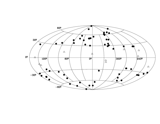
Figure 1: Aitoff projection of the 63 HIFLUGCS galaxy clusters in galactic coordinates (filled circles). Additionally shown are 11 clusters above the flux limit but with $|b_{\rm II}|<20.0\,\rm deg$ (open triangles).

3 Data Reduction and Analysis

This Section describes the derivation of the basic quantities in this work, e.g., count rates, fluxes, luminosities, and mass estimates for the galaxy clusters. These and other relevant cluster parameters are tabulated along with their uncertainties.

3.1 Flux Determination

Measuring the count rate of galaxy clusters is an important step in constructing a flux-limited cluster sample. The count rate determination performed here is based on the growth curve analysis method (Böhringer et al., 2000), with modifications adapted to the higher photon statistics available here. The main features of the method as well as the modifications are outlined below.

The instrument used is the ROSAT PSPC (Pfeffermann et al., 1987), with a low internal background ideally suited for this study which needs good signal to noise of the outer, low surface brightness regions of the clusters. Mainly pointed observations from the public archive at MPE have been used. If the cluster is extended beyond the PSPC field of view making a proper background determination difficult or if there is no pointed PSPC observation available, RASS data have been used. The ROSAT hard energy band (channels $52-201\approx 0.5-2.0\,{\rm keV}$) has been used for all count rate measurements because of the higher background in the soft band.

Two X-ray cluster centers are determined by finding the two-dimensional ‘center of mass’ of the photon distribution iteratively for an aperture radius of 3 and 7.5 arcmin around the starting position. The small aperture yields the center representing the position of the cluster’s peak emission and therefore probably indicates the position where the cluster’s potential well is deepest. This center is used for the regional selection, e.g. $|b_{\rm II}|\geq 20.0$. The more globally defined center with the larger aperture is used for the subsequent analysis tasks since for the mass determination it is most important to have a good estimate of the slope of the surface brightness profile in the outer parts of the cluster.

The background surface brightness is determined in a ring outside the cluster emission. To minimize the influence of discrete sources the ring is subdivided into twelve parts of equal area and a sigma clipping is performed. To determine the count rate the area around the global center is divided into concentric rings. For pointed observations 200 rings with a width of 15 arcsec each are used. Due to the lower photon statistics a width of 30 arcsec is used for RASS data and the number of rings depends on the field size extracted ($100-300$ rings for field sizes of $2\times 2\,\rm deg^{2}-8\times 8\,\rm deg^{2}$). Each photon is divided by the vignetting and deadtime corrected exposure time of the skypixel where it has been detected and these ratios are summed up in each ring yielding the ring count rate. From this value the background count rate for the respective ring area is subtracted yielding a source ring count rate. These individual source ring count rates are integrated with increasing radius yielding the (cumulative) source count rate for a given radius (Fig. 2). Obvious contaminating point sources have been excluded manually. The cut-out regions have then been assigned the average surface brightness of the ring. If a cluster has been found to be clearly made up of two components, for instance A3395n/s, these components have been treated separately. This procedure ensures that double clusters are not treated as a single entity for which spherical symmetry is assumed. For the same reason strong substructure has been excluded in the same manner as contaminating point sources. In this work the aim is to characterize all cluster properties consistently and homogeneously. Therefore if strong substructure is identified then it is excluded for the flux/luminosity and mass determination.

An outer significance radius of the cluster, $r_{\rm X}$, is determined at the position from where on the Poissonian 1-$\sigma$ error rises faster than the source count rate. Usually the source count rate settles into a nearly horizontal line for radii larger than $r_{\rm X}$. We have found, however, that in some cases the source count rate seems to increase or decrease roughly quadratically for radii larger than $r_{\rm X}$ indicating a possibly under- or overestimated background (Fig. 3). We therefore fitted a parabola of the form $y=mx^{2}+b$ to the source count rate for radii larger than $r_{\rm X}$ and corrected the measured background. An example for a corrected source count rate profile is shown in Fig. 4.

Figure 5 shows for the extended sample (106 clusters) that the difference between measured and corrected source count rate is generally very small. Nevertheless an inspection of each count rate profile has been performed, to decide whether the measured or corrected count rate is adopted as the final count rate, to avoid artificial corrections due to large scale variations of the background (especially in the large RASS fields). The count rates are given in Tab. 3.1.

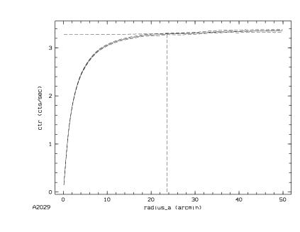
Figure 2: Cumulative source count rate as a function of radius (solid line) for the cluster A2029 (pointed observation). The vertical dashed line indicates the outer significance radius, $r_{\rm X}$. The dashed lines just above and below the source count rate indicate the 1-$\sigma$ Poissonian error bars.

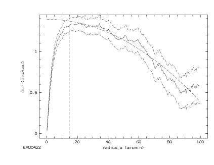
Figure 3: Cumulative source count rate as a function of radius for the cluster EXO0422, shown as an extreme example (RASS data). The parabolic dashed line indicates the best fit parabola for count rates larger than $r_{\rm X}$.

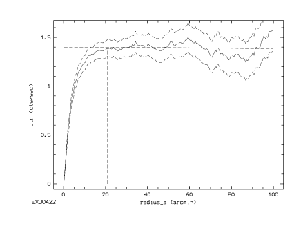
Figure 4: Corrected cumulative source count rate as a function of radius for the cluster EXO0422. The count rate correction is less than 5 %.

Figure 5: Comparison of measured and corrected source count rates for the extended sample of 106 galaxy clusters. The solid line indicates equality.

The conversion factor for the count rate to flux conversion depends on the hydrogen column density, $n_{\rm H}$, on the cluster gas temperature, $T_{\rm gas}$, on the cluster gas metallicity, on the cluster redshift, $z$, and on the respective detector responses for the two different PSPCs used. The $n_{\rm H}$ value is taken as the value inferred from 21 cm radio measurements for our galaxy at the projected cluster position (Dickey & Lockman 1990; included in the EXSAS software package, Zimmermann et al. 1998; photoelectric absorption cross sections are taken from Morrison & McCammon 1983). Gas temperatures have been estimated by compiling X-ray temperatures, $T_{\rm X}$, from the literature, giving preference to temperatures measured with the ASCA satellite. For clusters where no ASCA measured temperature has been available, $T_{\rm X}$ measured with previous X-ray satellites have been used. The X-ray temperatures and corresponding references are given in Tab. 3.2. For two clusters included in HIFLUGCS no measured temperature has been found in the literature and the $L_{\rm X}(<2\,h_{50}^{-1}\,{\rm Mpc})-T_{\rm X}$ relation of Markevitch (1998) has been used. The relation for non cooling flow corrected luminosities and cooling flow corrected/emission weighted temperatures has been chosen. Since the conversion from count rate to flux depends only weakly on $T_{\rm gas}$ in the ROSAT energy band for the relevant temperature range a cluster temperature $kT_{\rm gas}=4\,\rm keV$ has been assumed in a first step to determine $L_{\rm X}(<2\,h_{50}^{-1}\,{\rm Mpc})$ for the clusters where no gas temperature has been found in the literature. With this luminosity the gas temperature has been estimated. The metallicity is set to 0.35 times the solar value for all clusters (e.g., Arnaud et al., 1992). The redshifts have been compiled from the literature and are given in Tab. 3.1 together with the corresponding references. With these quantities and the count rates given in Tab. 3.1 fluxes in the observer rest frame energy range $0.1-2.4\,{\rm keV}$ have been calculated applying a modern version of a Raymond-Smith spectral code (Raymond & Smith, 1977). The results are listed in Tab. 3.1. The flux calculation has also been checked using XSPEC (Arnaud, 1996) by folding the model spectrum created with the parameters given above with the detector response and adjusting the normalization to reproduce the observed count rate. It is found that for 90 % of the clusters the deviation between the two results for the flux measurement is less than 1 %. Luminosities in the source rest frame energy range $0.1-2.4\,{\rm keV}$ have then been calculated within XSPEC by adjusting the normalization to reproduce the initial flux measurements.

The improvements of the flux determination performed here compared to the input catalogs in general are now summarized. 1) Due to the use of a high fraction of pointed observations the photon statistics is on average much better, e.g., for the 33 clusters contained in REFLEX and HIFLUGCS one finds a mean of 841 and 19580 source photons, respectively. Consequently the cluster emission has been traced out to larger radii for HIFLUGCS. 2) The higher photon statistics has allowed a proper exclusion of contaminating point sources (stars, AGN, etc.) and substructure, and the separation of double clusters. 3) An iterative background correction has been performed. 4) A measured X-ray temperature has been used for the flux calculation in most cases.

Simulations have shown that even for the HIFLUGCS clusters with the lowest number of photons the determined flux shows no significant trend with redshift in the relevant redshift range (Ikebe et al., 2001).

Table 3: Cluster properties

Cluster	R.A.	Dec.	$z$	$n_{\rm H}$	$C_{\rm X}$	$\Delta$	$r_{\rm X}$	$f_{\rm X}$	$L_{\rm X}$	$L_{\rm Bol}$	Obs	Ref
(1)	(2)	(3)	(4)	(5)	(6)	(7)	(8)	(9)	(10)	(11)	(12)	(13)
A0085	10.4632	$-9.3054$	0.0556	3.58	3.488	0.6	2.13	7.429	9.789	24.448	P	2
A0119	14.0649	$-1.2489$	0.0440	3.10	1.931	0.9	2.68	4.054	3.354	7.475	P	1
A0133	15.6736	$-21.8806$	0.0569	1.60	1.058	0.8	1.52	2.121	2.944	5.389	P	3
NGC507	20.9106	$33.2553$	0.0165	5.25	1.093	1.3	0.88	2.112	0.247	0.326	P	5
A0262	28.1953	$36.1528$	0.0161	5.52	4.366	3.8	1.48	9.348	1.040	1.533	R	6
A0400	44.4152	$6.0170$	0.0240	9.38	1.146	1.1	1.85	2.778	0.686	1.033	P	8
A0399	44.4684	$13.0462$	0.0715	10.58	1.306	5.4	3.18	3.249	7.070	17.803	R	6
A0401	44.7384	$13.5796$	0.0748	10.19	2.104	1.1	3.81	5.281	12.553	34.073	P	6
A3112	49.4912	$-44.2367$	0.0750	2.53	1.502	1.1	2.18	3.103	7.456	16.128	P	1
FORNAX	54.6686	$-35.3103$	0.0046	1.45	5.324	5.6	0.53	9.020	0.082	0.107	P+R	4
2A0335	54.6690	$9.9713$	0.0349	18.64	3.028	0.8	1.54	9.162	4.789	7.918	P	10
IIIZw54	55.3225	$15.4076$	0.0311	16.68	0.708	7.7	1.27	2.001	0.831	1.226	R	11
A3158	55.7282	$-53.6301$	0.0590	1.06	1.909	1.5	1.94	3.794	5.638	12.779	P	1
A0478	63.3554	$10.4661$	0.0900	15.27	1.827	0.6	3.12	5.151	17.690	49.335	P	6
NGC1550	64.9066	$2.4151$	0.0123	11.59	1.979	5.4	0.71	4.632	0.302	0.407	R	13
EXO0422	66.4637	$-8.5581$	0.0390	6.40	1.390	6.2	1.32	3.085	2.015	3.283	R	10
A3266	67.8410	$-61.4403$	0.0594	1.48	2.879	0.7	2.99	5.807	8.718	23.663	P	4
A0496	68.4091	$-13.2605$	0.0328	5.68	3.724	0.7	1.78	8.326	3.837	7.306	P	8
A3376	90.4835	$-39.9741$	0.0455	5.01	1.115	1.4	2.86	2.450	2.174	4.077	P	4
A3391	96.5925	$-53.6938$	0.0531	5.42	0.999	1.9	1.98	2.225	2.681	5.857	P	4
A3395s	96.6920	$-54.5453$	0.0498	8.49	0.836	3.8	1.45	2.009	2.131	4.471	P	4
A0576	110.3571	$55.7639$	0.0381	5.69	1.374	6.8	2.32	3.010	1.872	3.518	R	6
A0754	137.3338	$-9.6797$	0.0528	4.59	1.537	1.6	1.91	3.366	3.990	11.967	P	6
HYDRA-A	139.5239	$-12.0942$	0.0538	4.86	2.179	0.6	1.66	4.776	5.930	11.520	P	13
A1060	159.1784	$-27.5212$	0.0114	4.92	4.653	3.3	0.95	9.951	0.554	0.945	R	6
A1367	176.1903	$19.7030$	0.0216	2.55	2.947	0.8	1.55	6.051	1.206	2.140	P	8
MKW4	181.1124	$1.8962$	0.0200	1.86	1.173	1.7	1.23	2.268	0.390	0.543	P	10
ZwCl1215	184.4220	$3.6604$	0.0750	1.64	1.081	1.3	2.55	2.183	5.240	11.656	P	19
NGC4636	190.7084	$2.6880$	0.0037	1.75	3.102	7.2	0.39	4.085	0.023	0.027	R	13
A3526	192.1995	$-41.3087$	0.0103	8.25	11.655	2.2	1.64	27.189	1.241	2.238	R	15
A1644	194.2900	$-17.4029$	0.0474	5.33	1.853	5.1	1.85	4.030	3.876	7.882	R	8
A1650	194.6712	$-1.7572$	0.0845	1.54	1.218	6.6	3.17	2.405	7.308	17.955	R	6
A1651	194.8419	$-4.1947$	0.0860	1.71	1.254	1.2	2.03	2.539	8.000	18.692	P	22
COMA	194.9468	$27.9388$	0.0232	0.89	17.721	1.4	4.04	34.438	7.917	22.048	R	8
NGC5044	198.8530	$-16.3879$	0.0090	4.91	3.163	0.5	0.56	5.514	0.193	0.246	P	24
A1736	201.7238	$-27.1765$	0.0461	5.36	1.631	6.3	2.47	3.537	3.223	5.682	R	25
A3558	201.9921	$-31.5017$	0.0480	3.63	3.158	0.5	2.11	6.720	6.615	14.600	P	1
A3562	203.3984	$-31.6678$	0.0499	3.91	1.367	0.9	2.01	2.928	3.117	6.647	P	4
A3571	206.8692	$-32.8553$	0.0397	3.93	5.626	0.7	2.35	12.089	8.132	20.310	P	21
A1795	207.2201	$26.5944$	0.0616	1.20	3.132	0.3	2.14	6.270	10.124	27.106	P	6
A3581	211.8852	$-27.0153$	0.0214	4.26	1.603	3.2	0.64	3.337	0.657	0.926	P	28
MKW8	220.1596	$3.4717$	0.0270	2.60	1.255	8.4	1.90	2.525	0.789	1.355	R	29
A2029	227.7331	$5.7450$	0.0767	3.07	3.294	0.6	2.78	6.938	17.313	50.583	P	6
A2052	229.1846	$7.0211$	0.0348	2.90	2.279	1.0	1.14	4.713	2.449	4.061	P	6
MKW3S	230.4643	$7.7059$	0.0450	3.15	1.578	1.0	1.39	3.299	2.865	5.180	P	10
A2065	230.6096	$27.7120$	0.0721	2.84	1.227	6.1	3.09	2.505	5.560	12.271	R	6
A2063	230.7734	$8.6112$	0.0354	2.92	2.038	1.3	2.13	4.232	2.272	4.099	P	8
A2142	239.5824	$27.2336$	0.0899	4.05	2.888	0.9	3.09	6.241	21.345	64.760	P	6
A2147	240.5628	$15.9586$	0.0351	3.29	2.623	3.2	1.87	5.522	2.919	6.067	P	8
A2163	243.9433	$-6.1436$	0.2010	12.27	0.773	1.5	3.15	2.039	34.128	123.200	P	31
A2199	247.1586	$39.5477$	0.0302	0.84	5.535	1.8	2.37	10.642	4.165	7.904	R	8
A2204	248.1962	$5.5733$	0.1523	5.94	1.211	1.6	3.29	2.750	26.938	68.989	P	6
A2244	255.6749	$34.0578$	0.0970	2.07	1.034	2.1	2.64	2.122	8.468	21.498	P	6
A2256	255.9884	$78.6481$	0.0601	4.02	2.811	1.4	3.09	6.054	9.322	22.713	P	6
A2255	258.1916	$64.0640$	0.0800	2.51	0.976	1.2	3.22	2.022	5.506	13.718	P	6
A3667	303.1362	$-56.8419$	0.0560	4.59	3.293	0.7	2.81	7.201	9.624	24.233	P	1
S1101	348.4941	$-42.7268$	0.0580	1.85	1.237	0.9	1.64	2.485	3.597	5.939	P	35
A2589	350.9868	$16.7753$	0.0416	4.39	1.200	1.3	1.46	2.591	1.924	3.479	P	37
A2597	351.3318	$-12.1246$	0.0852	2.50	1.074	1.2	1.43	2.213	6.882	13.526	P	6
A2634	354.6201	$27.0269$	0.0312	5.17	1.096	1.6	1.79	2.415	1.008	1.822	P	6
A2657	356.2334	$9.1952$	0.0404	5.27	1.148	0.9	1.52	2.535	1.771	3.202	P	8
A4038	356.9322	$-28.1415$	0.0283	1.55	2.854	1.3	1.35	5.694	1.956	3.295	P	4
A4059	359.2541	$-34.7591$	0.0460	1.10	1.599	1.3	1.72	3.170	2.872	5.645	P	36
Clusters from the extended sample not included in HIFLUGCS.
A2734	2.8389	$-28.8539$	0.0620	1.84	0.710	2.5	1.74	1.434	2.365	4.357	P	1
A2877	17.4796	$-45.9225$	0.0241	2.10	0.801	1.2	1.06	1.626	0.405	0.714	P	4
NGC499	20.7971	$33.4587$	0.0147	5.25	0.313	2.5	0.30	0.479	0.045	0.051	P	5
AWM7	43.6229	$41.5781$	0.0172	9.21	7.007	2.0	1.58	16.751	2.133	3.882	R	7
PERSEUS	49.9455	$41.5150$	0.0183	15.69	40.723	0.8	3.30	113.731	16.286	40.310	R	9
S405	58.0078	$-82.2315$	0.0613	7.65	0.781	8.2	2.14	1.800	2.899	5.574	R	12
3C129	72.5602	$45.0256$	0.0223	67.89	1.512	5.6	1.61	10.566	2.242	4.996	R	10
A0539	79.1560	$6.4421$	0.0288	12.06	1.221	1.3	1.37	3.182	1.135	1.935	P	14
S540	85.0265	$-40.8431$	0.0358	3.53	0.788	5.0	0.84	1.611	0.887	1.353	R	4
A0548w	86.3785	$-25.9340$	0.0424	1.79	0.136	5.4	0.73	0.234	0.183	0.240	P	15
A0548e	87.1596	$-25.4692$	0.0410	1.88	0.771	1.8	2.12	1.551	1.117	1.870	P	15
A3395n	96.9005	$-54.4447$	0.0498	5.42	0.699	3.9	1.37	1.555	1.650	3.461	P	4
UGC03957	115.2481	$55.4319$	0.0340	4.59	0.936	6.0	0.94	1.975	0.980	1.531	R	16
PKS0745	116.8837	$-19.2955$	0.1028	43.49	1.268	1.0	2.44	6.155	27.565	70.604	P	17
A0644	124.3553	$-7.5159$	0.0704	5.14	1.799	1.0	4.02	3.994	8.414	22.684	P	6
S636	157.5151	$-35.3093$	0.0116	6.42	3.102	4.9	1.18	5.869	0.341	0.446	R	18
A1413	178.8271	$23.4051$	0.1427	1.62	0.636	1.6	2.39	1.289	11.090	28.655	P	6
M49	187.4437	$7.9956$	0.0044	1.59	1.259	1.0	0.27	1.851	0.015	0.019	P	15
A3528n	193.5906	$-29.0130$	0.0540	6.10	0.560	2.3	1.51	1.263	1.581	2.752	P	1
A3528s	193.6708	$-29.2254$	0.0551	6.10	0.756	1.6	1.35	1.703	2.224	3.746	P	20
A3530	193.9211	$-30.3451$	0.0544	6.00	0.438	2.8	1.55	0.987	1.252	2.317	P	21
A3532	194.3375	$-30.3698$	0.0539	5.96	0.797	1.8	1.64	1.797	2.235	4.483	P	21
A1689	197.8726	$-1.3408$	0.1840	1.80	0.712	1.1	2.36	1.454	20.605	60.707	P	23
A3560	203.1119	$-33.1355$	0.0495	3.92	0.714	2.5	2.00	1.519	1.601	2.701	P	26
A1775	205.4582	$26.3820$	0.0757	1.00	0.654	1.8	2.02	1.290	3.175	5.735	P	27
A1800	207.3408	$28.1038$	0.0748	1.18	0.610	7.9	1.98	1.183	2.840	5.337	R	28
A1914	216.5035	$37.8268$	0.1712	0.97	0.729	1.4	2.35	1.454	17.813	56.533	P	6
NGC5813	225.2994	$1.6981$	0.0064	4.19	0.976	6.7	0.17	1.447	0.025	0.029	R	13
NGC5846	226.6253	$1.6089$	0.0061	4.25	0.569	2.3	0.21	0.851	0.014	0.016	P	13
A2151w	241.1465	$17.7252$	0.0369	3.36	0.754	1.9	1.46	1.568	0.917	1.397	P	8
A3627	243.5546	$-60.8430$	0.0163	20.83	9.962	3.0	2.20	31.084	3.524	8.179	R	30
TRIANGUL	249.5758	$-64.3557$	0.0510	12.29	4.294	0.7	2.54	11.308	12.508	37.739	P	32
OPHIUCHU	258.1115	$-23.3634$	0.0280	20.14	11.642	2.0	2.29	35.749	11.953	37.391	R	33
ZwCl1742	266.0623	$32.9893$	0.0757	3.56	0.889	4.4	1.83	1.850	4.529	9.727	R	34
A2319	290.2980	$43.9484$	0.0564	8.77	5.029	1.0	3.57	12.202	16.508	47.286	P	6
A3695	308.6991	$-35.8135$	0.0890	3.56	0.836	9.2	2.58	1.739	5.882	12.715	R	1
IIZw108	318.4752	$2.5564$	0.0494	6.63	0.841	7.3	2.20	1.884	1.969	3.445	R	5
A3822	328.5438	$-57.8668$	0.0760	2.12	0.964	7.3	3.18	1.926	4.758	9.877	R	1
A3827	330.4869	$-59.9641$	0.0980	2.84	0.953	5.8	1.78	1.955	7.963	20.188	R	1
A3888	338.6255	$-37.7343$	0.1510	1.20	0.546	2.4	1.52	1.096	10.512	30.183	P	23
A3921	342.5019	$-64.4286$	0.0936	2.80	0.626	1.7	2.43	1.308	4.882	11.023	P	12
HCG94	349.3041	$18.7060$	0.0417	4.55	0.820	1.0	2.09	1.775	1.324	2.319	P	36
RXJ2344	356.0723	$-4.3776$	0.0786	3.54	0.653	1.4	1.61	1.385	3.661	7.465	P	12

Note. — Column (1) lists the cluster name. Names have been truncated to at most eight characters to preserve the compactness of the table. Columns (2) and (3) give the equatorial coordinates of the cluster center used for the regional selection for the epoch J2000 in decimal degrees. Column (4) gives the heliocentric cluster redshift. Column (5) lists the column density of neutral galactic hydrogen in units of $10^{20}\,\rm atoms\,cm^{-2}$. Column (6) gives the count rate in the channel range 52–201 which corresponds to about (the energy resolution of the PSPC is limited) the energy range $0.5-2.0\,{\rm keV}$ in units of ${\rm cts\,s^{-1}}$. Column (7) lists the relative 1-$\sigma$ Poissonian error of the count rate, the flux, and the luminosity in percent. Column (8) gives the significance radius in $h_{50}^{-1}\,{\rm Mpc}$. Column (9) lists the flux in the energy range $0.1-2.4\,{\rm keV}$ in units of $10^{-11}\,{\rm ergs\,s^{-1}\,cm^{-2}}$. Column (10) gives the luminosity in the energy range $0.1-2.4\,{\rm keV}$ in units of $h_{50}^{-2}\,10^{44}\,{\rm ergs\,s^{-1}}$. Column (11) gives the bolometric luminosity (energy range $0.01-40\,{\rm keV}$) in units of $h_{50}^{-2}\,10^{44}\,{\rm ergs\,s^{-1}}$. Column (12) indicates whether a RASS (R) or a pointed (P) ROSAT PSPC observation has been used. Column (13) lists the code for the redshift reference decoded below.

References. — (1) Katgert et al. 1996. (2) Mazure et al. 1996. (3) Median of 9 galaxy redshifts compiled from Lauberts & Valentijn 1989; Merrifield & Kent 1991; Loveday et al. 1996; Way et al. 1998. (4) Abell et al. 1989. (5) Huchra et al. 1999. (6) Struble & Rood 1987. (7) dell’Antonio et al. 1994. (8) Zabludoff et al. 1993. (9) Poulain et al. 1992. (10) NED Team 1992. (11) Böhringer et al. 2000. (12) De Grandi et al. 1999. (13) de Vaucouleurs et al. 1991. (14) Zabludoff et al. 1990. (15) den Hartog & Katgert 1996. (16) Michel & Huchra 1988. (17) Yan & Cohen 1995. (18) Garcia 1995. (19) Ebeling et al. 1998. (20) Median of 8 galaxy redshifts compiled from de Vaucouleurs et al. 1991; Quintana et al. 1995; Katgert et al. 1998. (21) Vettolani et al. 1990. (22) Allen et al. 1992. (23) Teague et al. 1990. (24) da Costa et al. 1998. (25) Dressler & Shectman 1988. (26) Melnick & Moles 1987. (27) Median of 13 galaxy redshifts compiled from Kirshner et al. 1983; Zabludoff et al. 1990; NED Team 1992; Davoust & Considere 1995; Oegerle et al. 1995. (28) Postman et al. 1992. (29) Andersen & Owen 1994. (30) Kraan-Korteweg et al. 1996. (31) Elbaz et al. 1995. (32) Edge & Stewart 1991a. (33) Lahav et al. 1989. (34) Ulrich 1976. (35) Stocke et al. 1991. (36) Hickson et al. 1992. (37) Beers et al. 1991.

3.2 Mass Determination

A parametric description of the cluster gas density profile has been derived using the standard $\beta$ model (e.g., Cavaliere & Fusco-Femiano, 1976; Gorenstein et al., 1978; Jones & Forman, 1984). Assuming spherical symmetry the model

$$S_{\rm X}(R)=S_{0}\left(1+\frac{R^{2}}{r_{\rm c}^{2}}\right)^{-3\beta+\frac{1}{2}}+B$$ (1)

is fitted to the measured surface brightness profile (ring count rates per ring area), where $R$ denotes the projected distance from the cluster center. This yields values for the core radius, $r_{\rm c}$, the $\beta$ parameter, and the normalization, $S_{0}$ (and also a fitted value for the background surface brightness, $B$, since the fit is performed on the non background subtracted data). The fit values have been used to construct the radial gas density distribution

$$\rho_{\rm gas}(r)=\rho_{0}\left(1+\frac{r^{2}}{r_{\rm c}^{2}}\right)^{-\frac{3}{2}\beta}.$$ (2)

The gravitational cluster mass, $M_{\rm tot}$, has been determined assuming the intracluster gas to be in hydrostatic equilibrium and isothermal. Using (2) and the ideal gas equation under these assumptions leads to

$$M_{\rm tot}(<r)=\frac{3kT_{\rm gas}r^{3}\beta}{\mu m_{\rm p}G}\left(\frac{1}{r^{2}+r_{\rm c}^{2}}\right),$$ (3)

where $\mu\,(=0.61)$ represents the mean molecular weight, $m_{\rm p}$ the proton mass, and $G$ the gravitational constant. Combined $N$-body/hydrodynamic cluster simulations have shown that this method generally gives unbiased results with an uncertainty of 14–29 % (e.g., Schindler, 1996a; Evrard et al., 1996). Currently there are contradictory measurements concerning the general presence of gas temperature gradients in clusters (e.g., Fukazawa, 1997; Markevitch et al., 1998; Irwin et al., 1999; White, 2000; Irwin & Bregman, 2000). If there is a systematic trend in the sense that the gas temperature decreases with increasing radius in the outer cluster parts similar to that found by Markevitch et al. then the isothermal assumption leads to an overestimation of the cluster mass of about 30 % at about 6 core radii (Markevitch et al., 1998). Finoguenov et al. (2001) determined masses by employing the assumption of isothermality and also using measured cluster gas temperature profiles. A comparison for 38 clusters included in their sample indicates that the latter masses are on average a factor of 0.80 smaller than the isothermal masses within $r_{200}$ (this radius is defined in the next paragraph). Until the final answer on this issue is given by XMM-Newton, we retain the isothermal assumption. The influence of a possible overestimation of the cluster mass on the determination of cosmological parameters is investigated in Sect. 5.3.2.

Having determined the integrated mass as a function of radius, a physically meaningful fiducial radius for the mass measurement has to be defined. The radii commonly used are either the Abell radius, $r_{200}$, or $r_{500}$. The Abell radius is fixed at $r_{\rm A}\equiv 3\,h_{50}^{-1}\,{\rm Mpc}$. The radius $r_{200}$ ($r_{500}$) is the radius within which the mean gravitational mass density $\langle\rho_{\rm tot}\rangle=200\,(500)\,\rho_{\rm c}$. The critical cosmic matter density is defined as $\rho_{\rm c}\equiv 3\,H^{2}/(8\,\pi\,G)$, where $H^{2}=H^{2}_{0}\,E(z)^{2}$ and $E(z)=[\Omega_{\rm m}(1+z)^{3}+\Omega_{\rm k}(1+z)^{2}+\Omega_{\Lambda}]^{1/2}$. It has been shown that a correction for redshift is not necessary for the nearby clusters included in HIFLUGCS (Finoguenov et al., 2001) and we use the zero redshift value for all calculations, i.e. $\rho_{\rm c}=4.6975\times 10^{-30}\rm g\,cm^{-3}$, unless noted otherwise. Nevertheless the influence of this approximation is tested in Sect. 5.3.2 for the model ($\Omega_{\rm m}=1,\Omega_{\Lambda}=0$), where evolution is strong.

In order to treat clusters of different size in a homogeneous way we determine the cluster mass at a characteristic density but also give the mass determined formally at a fixed radius for comparison. Spherical collapse models predict a cluster virial density $\langle\rho_{\rm vir}\rangle\approx 178\,\rho_{\rm c}$ for ($\Omega_{\rm m}=1,\Omega_{\Lambda}=0$), so a pragmatic approximation to the virial mass is to use $r_{200}$ as the outer boundary. Simulations performed by Evrard et al. (1996) have shown, however, that isothermal X-ray mass measurements may be biased towards high masses for $r>r_{500}$. Furthermore for most of the clusters in HIFLUGCS (86 %) up to $r_{500}$ no extrapolation outside the significantly detected cluster emission is necessary, i.e. $r_{500}<r_{\rm X}$, whereas the fraction is lower for $r_{200}$ (25 %) and $r_{\rm A}$ (17 %). In summary the most accurate results are expected for $M_{\rm tot}(<r_{500})\equiv M_{500}$, but for a comparison to predicted mass functions $M_{200}$ is the more appropriate value (Sect. 5.3.2). Results for all determined masses and their corresponding radii are given in Tab. 3.2. Masses for the cluster gas will be given in a subsequent paper.

A major source of uncertainty comes from the temperature measurements. However, this (statistical) error is less than 5 % for one third of the clusters, therefore also other sources of error have to be taken into account, in particular one cannot neglect the uncertainties of the fit parameter values when assessing the statistical errors of the mass measurements. Therefore mass errors have been calculated by varying the fit parameter values, $\beta$ and $r_{\rm c}$, along their 68 % confidence level error ellipse and using the upper and lower bound of the quoted temperature ranges. The statistical mass error range has then been defined between the maximum and minimum mass. Note that a simple error propagation applied to (3) would underestimate the uncertainty of $M_{200}$ and $M_{500}$, since $r_{200}$ and $r_{500}$ also depend on $T_{\rm gas}$, $\beta$, and (weakly) $r_{\rm c}$. The individual mass errors have been used in subsequent calculations, unless noted otherwise. A mean statistical error of 23 % for clusters included in HIFLUGCS and a mean error of 27 % for the extended sample has been found.

Table 4: Cluster properties

Cluster	$\beta$	$r_{\rm c}$	$T_{\rm X}$	$M_{500}$	$r_{500}$	$M_{200}$	$r_{200}$	$M_{\rm A}$	Ref
(1)	(2)	(3)	(4)	(5)	(6)	(7)	(8)	(9)	(10)
A0085	$0.532^{+0.004}_{-0.004}$	$83^{+3}_{-3}$	$6.90^{+0.40}_{-0.40}$	$6.84^{+0.66}_{-0.66}$	$1.68^{+0.05}_{-0.06}$	$10.80^{+1.12}_{-1.04}$	$2.66^{+0.09}_{-0.09}$	12.21	1
A0119	$0.675^{+0.026}_{-0.023}$	$501^{+28}_{-26}$	$5.60^{+0.30}_{-0.30}$	$6.23^{+0.92}_{-0.76}$	$1.63^{+0.08}_{-0.07}$	$10.76^{+1.50}_{-1.39}$	$2.66^{+0.11}_{-0.13}$	12.24	1
A0133	$0.530^{+0.004}_{-0.004}$	$45^{+2}_{-2}$	$3.80^{+2.00}_{-0.90}$	$2.78^{+2.51}_{-0.95}$	$1.24^{+0.30}_{-0.16}$	$4.41^{+4.00}_{-1.52}$	$1.97^{+0.47}_{-0.27}$	6.71	9
NGC507	$0.444^{+0.005}_{-0.005}$	$19^{+1}_{-1}$	$1.26^{+0.07}_{-0.07}$	$0.41^{+0.04}_{-0.04}$	$0.66^{+0.02}_{-0.02}$	$0.64^{+0.07}_{-0.06}$	$1.04^{+0.04}_{-0.04}$	1.86	2
A0262	$0.443^{+0.018}_{-0.017}$	$42^{+12}_{-10}$	$2.15^{+0.06}_{-0.06}$	$0.90^{+0.10}_{-0.09}$	$0.86^{+0.03}_{-0.03}$	$1.42^{+0.15}_{-0.13}$	$1.35^{+0.05}_{-0.04}$	3.17	2
A0400	$0.534^{+0.014}_{-0.013}$	$154^{+9}_{-9}$	$2.31^{+0.14}_{-0.14}$	$1.28^{+0.17}_{-0.15}$	$0.96^{+0.04}_{-0.04}$	$2.07^{+0.30}_{-0.25}$	$1.53^{+0.08}_{-0.06}$	4.10	2
A0399	$0.713^{+0.137}_{-0.095}$	$450^{+132}_{-100}$	$7.00^{+0.40}_{-0.40}$	$10.00^{+3.73}_{-2.48}$	$1.91^{+0.21}_{-0.18}$	$16.64^{+6.61}_{-4.32}$	$3.07^{+0.36}_{-0.30}$	16.24	1
A0401	$0.613^{+0.010}_{-0.010}$	$246^{+11}_{-10}$	$8.00^{+0.40}_{-0.40}$	$10.27^{+1.08}_{-0.93}$	$1.92^{+0.07}_{-0.05}$	$16.59^{+1.62}_{-1.62}$	$3.07^{+0.09}_{-0.10}$	16.21	1
A3112	$0.576^{+0.006}_{-0.006}$	$61^{+3}_{-3}$	$5.30^{+0.70}_{-1.00}$	$5.17^{+1.17}_{-1.45}$	$1.53^{+0.11}_{-0.16}$	$8.22^{+1.79}_{-2.31}$	$2.43^{+0.16}_{-0.25}$	10.16	1
FORNAX	$0.804^{+0.098}_{-0.084}$	$174^{+17}_{-15}$	$1.20^{+0.04}_{-0.04}$	$0.87^{+0.22}_{-0.16}$	$0.84^{+0.07}_{-0.06}$	$1.42^{+0.36}_{-0.27}$	$1.35^{+0.11}_{-0.09}$	3.20	2
2A0335	$0.575^{+0.004}_{-0.003}$	$33^{+1}_{-1}$	$3.01^{+0.07}_{-0.07}$	$2.21^{+0.10}_{-0.09}$	$1.15^{+0.02}_{-0.02}$	$3.51^{+0.16}_{-0.15}$	$1.83^{+0.03}_{-0.03}$	5.76	2
IIIZw54	$0.887^{+0.320}_{-0.151}$	$289^{+124}_{-73}$	($2.16^{+0.35}_{-0.30}$)	$2.36^{+2.22}_{-0.90}$	$1.18^{+0.29}_{-0.17}$	$3.93^{+3.83}_{-1.54}$	$1.89^{+0.48}_{-0.29}$	6.32	11
A3158	$0.661^{+0.025}_{-0.022}$	$269^{+20}_{-19}$	$5.77^{+0.10}_{-0.05}$	$7.00^{+0.52}_{-0.42}$	$1.69^{+0.04}_{-0.03}$	$11.29^{+0.95}_{-0.68}$	$2.69^{+0.08}_{-0.06}$	12.61	3
A0478	$0.613^{+0.004}_{-0.004}$	$98^{+2}_{-2}$	$8.40^{+0.80}_{-1.40}$	$11.32^{+1.78}_{-2.81}$	$1.99^{+0.10}_{-0.18}$	$17.89^{+2.95}_{-4.35}$	$3.13^{+0.18}_{-0.27}$	17.12	1
NGC1550	$0.554^{+0.049}_{-0.037}$	$45^{+15}_{-11}$	$1.43^{+0.04}_{-0.03}$	$0.69^{+0.12}_{-0.09}$	$0.78^{+0.04}_{-0.04}$	$1.09^{+0.20}_{-0.14}$	$1.23^{+0.07}_{-0.06}$	2.64	5
EXO0422	$0.722^{+0.104}_{-0.071}$	$142^{+40}_{-30}$	$2.90^{+0.90}_{-0.60}$	$2.89^{+2.39}_{-1.14}$	$1.26^{+0.28}_{-0.19}$	$4.63^{+3.84}_{-1.82}$	$2.00^{+0.44}_{-0.31}$	6.96	9
A3266	$0.796^{+0.020}_{-0.019}$	$564^{+21}_{-20}$	$8.00^{+0.50}_{-0.50}$	$14.17^{+1.94}_{-1.84}$	$2.14^{+0.09}_{-0.10}$	$23.76^{+3.23}_{-2.91}$	$3.45^{+0.15}_{-0.14}$	20.47	1
A0496	$0.484^{+0.003}_{-0.003}$	$30^{+1}_{-1}$	$4.13^{+0.08}_{-0.08}$	$2.76^{+0.11}_{-0.11}$	$1.24^{+0.02}_{-0.02}$	$4.35^{+0.18}_{-0.17}$	$1.96^{+0.03}_{-0.03}$	6.66	2
A3376	$1.054^{+0.101}_{-0.083}$	$755^{+69}_{-60}$	$4.00^{+0.40}_{-0.40}$	$6.32^{+2.11}_{-1.59}$	$1.64^{+0.17}_{-0.15}$	$11.96^{+3.82}_{-2.98}$	$2.75^{+0.26}_{-0.25}$	13.20	1
A3391	$0.579^{+0.026}_{-0.024}$	$234^{+24}_{-22}$	$5.40^{+0.60}_{-0.60}$	$5.18^{+1.31}_{-1.08}$	$1.53^{+0.12}_{-0.11}$	$8.41^{+2.13}_{-1.81}$	$2.44^{+0.19}_{-0.19}$	10.35	1
A3395s	$0.964^{+0.275}_{-0.167}$	$604^{+173}_{-118}$	$5.00^{+0.30}_{-0.30}$	$8.82^{+4.79}_{-2.61}$	$1.83^{+0.29}_{-0.20}$	$15.34^{+8.79}_{-4.74}$	$2.99^{+0.49}_{-0.35}$	15.42	1
A0576	$0.825^{+0.432}_{-0.185}$	$394^{+221}_{-125}$	$4.02^{+0.07}_{-0.07}$	$5.36^{+4.42}_{-1.66}$	$1.55^{+0.34}_{-0.18}$	$8.96^{+8.01}_{-2.91}$	$2.50^{+0.60}_{-0.31}$	10.86	3
A0754	$0.698^{+0.027}_{-0.024}$	$239^{+17}_{-16}$	$9.50^{+0.70}_{-0.40}$	$16.37^{+2.91}_{-1.84}$	$2.25^{+0.13}_{-0.09}$	$26.19^{+4.45}_{-2.95}$	$3.57^{+0.18}_{-0.15}$	21.94	1
HYDRA-A	$0.573^{+0.003}_{-0.003}$	$50^{+1}_{-1}$	$4.30^{+0.40}_{-0.40}$	$3.76^{+0.58}_{-0.55}$	$1.38^{+0.07}_{-0.07}$	$5.94^{+0.91}_{-0.84}$	$2.17^{+0.11}_{-0.10}$	8.21	1
A1060	$0.607^{+0.040}_{-0.034}$	$94^{+15}_{-13}$	$3.24^{+0.06}_{-0.06}$	$2.66^{+0.34}_{-0.28}$	$1.23^{+0.05}_{-0.04}$	$4.24^{+0.55}_{-0.47}$	$1.95^{+0.08}_{-0.08}$	6.54	2
A1367	$0.695^{+0.035}_{-0.032}$	$383^{+24}_{-22}$	$3.55^{+0.08}_{-0.08}$	$3.34^{+0.36}_{-0.32}$	$1.32^{+0.05}_{-0.04}$	$5.69^{+0.63}_{-0.56}$	$2.14^{+0.08}_{-0.07}$	8.08	2
MKW4	$0.440^{+0.004}_{-0.005}$	$11^{+1}_{-1}$	$1.71^{+0.09}_{-0.09}$	$0.64^{+0.06}_{-0.06}$	$0.76^{+0.02}_{-0.03}$	$1.00^{+0.10}_{-0.09}$	$1.20^{+0.04}_{-0.03}$	2.51	2
ZwCl1215	$0.819^{+0.038}_{-0.034}$	$431^{+28}_{-25}$	($5.58^{+0.89}_{-0.78}$)	$8.79^{+3.00}_{-2.29}$	$1.83^{+0.19}_{-0.18}$	$14.52^{+4.92}_{-3.67}$	$2.93^{+0.30}_{-0.27}$	14.91	11
NGC4636	$0.491^{+0.032}_{-0.027}$	$6^{+3}_{-2}$	$0.76^{+0.01}_{-0.01}$	$0.22^{+0.03}_{-0.02}$	$0.53^{+0.02}_{-0.02}$	$0.35^{+0.04}_{-0.04}$	$0.85^{+0.03}_{-0.03}$	1.24	4
A3526	$0.495^{+0.011}_{-0.010}$	$37^{+5}_{-4}$	$3.68^{+0.06}_{-0.06}$	$2.39^{+0.15}_{-0.13}$	$1.18^{+0.02}_{-0.02}$	$3.78^{+0.23}_{-0.18}$	$1.87^{+0.04}_{-0.03}$	6.07	2
A1644	$0.579^{+0.111}_{-0.074}$	$300^{+128}_{-92}$	$4.70^{+0.90}_{-0.70}$	$4.10^{+2.64}_{-1.41}$	$1.42^{+0.26}_{-0.18}$	$6.73^{+4.54}_{-2.38}$	$2.27^{+0.43}_{-0.31}$	8.98	10
A1650	$0.704^{+0.131}_{-0.081}$	$281^{+104}_{-71}$	$6.70^{+0.80}_{-0.80}$	$9.62^{+4.91}_{-2.92}$	$1.88^{+0.28}_{-0.21}$	$15.60^{+8.08}_{-4.85}$	$3.01^{+0.45}_{-0.35}$	15.56	1
A1651	$0.643^{+0.014}_{-0.013}$	$181^{+10}_{-10}$	$6.10^{+0.40}_{-0.40}$	$7.45^{+1.00}_{-0.95}$	$1.73^{+0.07}_{-0.08}$	$11.91^{+1.60}_{-1.52}$	$2.75^{+0.12}_{-0.13}$	13.01	1
COMA	$0.654^{+0.019}_{-0.021}$	$344^{+22}_{-21}$	$8.38^{+0.34}_{-0.34}$	$11.99^{+1.28}_{-1.29}$	$2.03^{+0.07}_{-0.08}$	$19.38^{+2.08}_{-1.97}$	$3.22^{+0.11}_{-0.11}$	18.01	2
NGC5044	$0.524^{+0.002}_{-0.003}$	$11^{+1}_{-1}$	$1.07^{+0.01}_{-0.01}$	$0.41^{+0.01}_{-0.01}$	$0.66^{+0.01}_{-0.01}$	$0.65^{+0.01}_{-0.01}$	$1.04^{+0.01}_{-0.01}$	1.87	2
A1736	$0.542^{+0.147}_{-0.092}$	$374^{+178}_{-130}$	$3.50^{+0.40}_{-0.40}$	$2.19^{+1.23}_{-0.74}$	$1.15^{+0.18}_{-0.15}$	$3.78^{+2.41}_{-1.34}$	$1.87^{+0.34}_{-0.25}$	6.22	1
A3558	$0.580^{+0.006}_{-0.005}$	$224^{+5}_{-5}$	$5.50^{+0.40}_{-0.40}$	$5.37^{+0.70}_{-0.64}$	$1.55^{+0.07}_{-0.06}$	$8.64^{+1.12}_{-1.03}$	$2.46^{+0.10}_{-0.10}$	10.56	1
A3562	$0.472^{+0.006}_{-0.006}$	$99^{+5}_{-5}$	$5.16^{+0.16}_{-0.16}$	$3.68^{+0.24}_{-0.23}$	$1.37^{+0.03}_{-0.03}$	$5.83^{+0.38}_{-0.36}$	$2.16^{+0.05}_{-0.04}$	8.10	3
A3571	$0.613^{+0.010}_{-0.010}$	$181^{+7}_{-7}$	$6.90^{+0.20}_{-0.20}$	$8.33^{+0.56}_{-0.53}$	$1.79^{+0.04}_{-0.04}$	$13.31^{+0.90}_{-0.85}$	$2.85^{+0.06}_{-0.06}$	14.04	1
A1795	$0.596^{+0.003}_{-0.002}$	$78^{+1}_{-1}$	$7.80^{+1.00}_{-1.00}$	$9.75^{+2.01}_{-1.90}$	$1.89^{+0.12}_{-0.14}$	$15.39^{+3.17}_{-2.92}$	$2.99^{+0.19}_{-0.20}$	15.46	1
A3581	$0.543^{+0.024}_{-0.022}$	$35^{+5}_{-4}$	$1.83^{+0.04}_{-0.04}$	$0.96^{+0.09}_{-0.09}$	$0.87^{+0.02}_{-0.03}$	$1.52^{+0.16}_{-0.13}$	$1.38^{+0.05}_{-0.04}$	3.30	5
MKW8	$0.511^{+0.098}_{-0.059}$	$107^{+70}_{-42}$	$3.29^{+0.23}_{-0.22}$	$2.10^{+0.86}_{-0.52}$	$1.14^{+0.13}_{-0.10}$	$3.33^{+1.45}_{-0.83}$	$1.79^{+0.24}_{-0.17}$	5.60	5
A2029	$0.582^{+0.004}_{-0.004}$	$83^{+2}_{-2}$	$9.10^{+1.00}_{-1.00}$	$11.82^{+2.14}_{-1.99}$	$2.01^{+0.11}_{-0.12}$	$18.79^{+3.40}_{-3.17}$	$3.20^{+0.18}_{-0.19}$	17.62	1
A2052	$0.526^{+0.005}_{-0.005}$	$37^{+2}_{-2}$	$3.03^{+0.04}_{-0.04}$	$1.95^{+0.07}_{-0.06}$	$1.10^{+0.02}_{-0.01}$	$3.10^{+0.09}_{-0.11}$	$1.75^{+0.01}_{-0.02}$	5.30	3
MKW3S	$0.581^{+0.008}_{-0.007}$	$66^{+3}_{-3}$	$3.70^{+0.20}_{-0.20}$	$3.06^{+0.32}_{-0.30}$	$1.29^{+0.05}_{-0.04}$	$4.84^{+0.51}_{-0.47}$	$2.03^{+0.07}_{-0.07}$	7.16	1
A2065	$1.162^{+0.734}_{-0.282}$	$690^{+360}_{-186}$	$5.50^{+0.40}_{-0.40}$	$13.44^{+16.12}_{-5.17}$	$2.10^{+0.63}_{-0.31}$	$23.37^{+29.87}_{-9.42}$	$3.43^{+1.09}_{-0.54}$	20.21	1
A2063	$0.561^{+0.011}_{-0.011}$	$110^{+7}_{-6}$	$3.68^{+0.11}_{-0.11}$	$2.84^{+0.23}_{-0.19}$	$1.25^{+0.04}_{-0.03}$	$4.54^{+0.36}_{-0.31}$	$1.99^{+0.06}_{-0.04}$	6.86	2
A2142	$0.591^{+0.006}_{-0.006}$	$154^{+6}_{-6}$	$9.70^{+1.50}_{-1.10}$	$13.29^{+3.45}_{-2.41}$	$2.10^{+0.17}_{-0.14}$	$21.04^{+5.46}_{-3.69}$	$3.31^{+0.26}_{-0.20}$	19.05	1
A2147	$0.444^{+0.071}_{-0.046}$	$238^{+103}_{-65}$	$4.91^{+0.28}_{-0.28}$	$2.99^{+0.92}_{-0.63}$	$1.28^{+0.12}_{-0.10}$	$4.84^{+1.64}_{-1.03}$	$2.03^{+0.21}_{-0.15}$	7.21	2
A2163	$0.796^{+0.030}_{-0.028}$	$519^{+31}_{-29}$	$13.29^{+0.64}_{-0.64}$	$31.85^{+4.24}_{-3.74}$	$2.81^{+0.12}_{-0.11}$	$51.99^{+6.96}_{-6.13}$	$4.49^{+0.19}_{-0.18}$	34.18	3
A2199	$0.655^{+0.019}_{-0.021}$	$139^{+10}_{-10}$	$4.10^{+0.08}_{-0.08}$	$4.21^{+0.33}_{-0.29}$	$1.43^{+0.04}_{-0.03}$	$6.73^{+0.52}_{-0.51}$	$2.27^{+0.06}_{-0.06}$	8.92	2
A2204	$0.597^{+0.008}_{-0.007}$	$67^{+3}_{-3}$	$7.21^{+0.25}_{-0.25}$	$8.67^{+0.67}_{-0.57}$	$1.82^{+0.05}_{-0.04}$	$13.79^{+0.96}_{-1.00}$	$2.89^{+0.06}_{-0.08}$	14.34	3
A2244	$0.607^{+0.016}_{-0.015}$	$126^{+11}_{-10}$	$7.10^{+5.00}_{-2.20}$	$8.65^{+11.47}_{-3.89}$	$1.82^{+0.59}_{-0.33}$	$13.78^{+18.02}_{-6.20}$	$2.89^{+0.92}_{-0.52}$	14.33	10
A2256	$0.914^{+0.054}_{-0.047}$	$587^{+40}_{-37}$	$6.60^{+0.40}_{-0.40}$	$12.83^{+2.38}_{-2.00}$	$2.07^{+0.12}_{-0.11}$	$21.81^{+4.07}_{-3.54}$	$3.36^{+0.19}_{-0.20}$	19.34	1
A2255	$0.797^{+0.033}_{-0.030}$	$593^{+35}_{-32}$	$6.87^{+0.20}_{-0.20}$	$10.90^{+1.15}_{-0.95}$	$1.96^{+0.07}_{-0.05}$	$18.65^{+2.01}_{-1.67}$	$3.18^{+0.11}_{-0.09}$	17.54	3
A3667	$0.541^{+0.008}_{-0.008}$	$279^{+10}_{-10}$	$7.00^{+0.60}_{-0.60}$	$6.88^{+1.08}_{-1.02}$	$1.68^{+0.08}_{-0.09}$	$11.19^{+1.76}_{-1.65}$	$2.69^{+0.13}_{-0.14}$	12.50	1
S1101	$0.639^{+0.006}_{-0.007}$	$56^{+2}_{-2}$	$3.00^{+1.20}_{-0.70}$	$2.58^{+1.76}_{-0.88}$	$1.22^{+0.23}_{-0.16}$	$4.08^{+2.78}_{-1.39}$	$1.92^{+0.36}_{-0.25}$	6.38	9
A2589	$0.596^{+0.013}_{-0.012}$	$118^{+8}_{-7}$	$3.70^{+2.20}_{-1.10}$	$3.14^{+3.44}_{-1.35}$	$1.29^{+0.37}_{-0.22}$	$5.01^{+5.41}_{-2.15}$	$2.06^{+0.56}_{-0.35}$	7.33	9
A2597	$0.633^{+0.008}_{-0.008}$	$58^{+2}_{-2}$	$4.40^{+0.40}_{-0.70}$	$4.52^{+0.72}_{-1.11}$	$1.47^{+0.07}_{-0.14}$	$7.14^{+1.14}_{-1.72}$	$2.31^{+0.11}_{-0.20}$	9.27	1
A2634	$0.640^{+0.051}_{-0.043}$	$364^{+44}_{-39}$	$3.70^{+0.28}_{-0.28}$	$3.15^{+0.78}_{-0.60}$	$1.29^{+0.10}_{-0.09}$	$5.35^{+1.34}_{-1.04}$	$2.10^{+0.17}_{-0.14}$	7.77	2
A2657	$0.556^{+0.008}_{-0.007}$	$119^{+5}_{-5}$	$3.70^{+0.30}_{-0.30}$	$2.83^{+0.43}_{-0.39}$	$1.25^{+0.06}_{-0.06}$	$4.52^{+0.68}_{-0.62}$	$1.99^{+0.10}_{-0.09}$	6.84	1
A4038	$0.541^{+0.009}_{-0.008}$	$59^{+4}_{-4}$	$3.15^{+0.03}_{-0.03}$	$2.16^{+0.09}_{-0.08}$	$1.14^{+0.02}_{-0.02}$	$3.41^{+0.14}_{-0.11}$	$1.80^{+0.03}_{-0.01}$	5.67	3
A4059	$0.582^{+0.010}_{-0.010}$	$90^{+5}_{-5}$	$4.40^{+0.30}_{-0.30}$	$3.95^{+0.52}_{-0.48}$	$1.40^{+0.06}_{-0.06}$	$6.30^{+0.83}_{-0.76}$	$2.22^{+0.09}_{-0.09}$	8.52	1
Clusters from the extended sample not included in HIFLUGCS.
A2734	$0.624^{+0.034}_{-0.029}$	$212^{+26}_{-23}$	($3.85^{+0.62}_{-0.54}$)	$3.49^{+1.25}_{-0.89}$	$1.34^{+0.15}_{-0.12}$	$5.67^{+1.98}_{-1.48}$	$2.14^{+0.22}_{-0.21}$	7.97	11
A2877	$0.566^{+0.029}_{-0.025}$	$190^{+19}_{-17}$	$3.50^{+2.20}_{-1.10}$	$2.61^{+3.32}_{-1.24}$	$1.22^{+0.39}_{-0.23}$	$4.24^{+5.28}_{-2.00}$	$1.95^{+0.60}_{-0.38}$	6.57	10
NGC499	$0.722^{+0.034}_{-0.030}$	$24^{+2}_{-2}$	$0.72^{+0.03}_{-0.02}$	$0.36^{+0.05}_{-0.04}$	$0.63^{+0.03}_{-0.02}$	$0.58^{+0.08}_{-0.06}$	$1.00^{+0.04}_{-0.04}$	1.73	4
AWM7	$0.671^{+0.027}_{-0.025}$	$173^{+18}_{-15}$	$3.75^{+0.09}_{-0.09}$	$3.79^{+0.38}_{-0.32}$	$1.38^{+0.05}_{-0.04}$	$6.08^{+0.62}_{-0.52}$	$2.19^{+0.08}_{-0.06}$	8.35	2
PERSEUS	$0.540^{+0.006}_{-0.004}$	$64^{+2}_{-2}$	$6.79^{+0.12}_{-0.12}$	$6.84^{+0.29}_{-0.26}$	$1.68^{+0.02}_{-0.02}$	$10.80^{+0.46}_{-0.41}$	$2.66^{+0.04}_{-0.04}$	12.20	2
S405	$0.664^{+0.263}_{-0.133}$	$459^{+262}_{-159}$	($4.21^{+0.67}_{-0.59}$)	$3.91^{+3.56}_{-1.57}$	$1.40^{+0.33}_{-0.22}$	$6.75^{+6.80}_{-2.81}$	$2.27^{+0.60}_{-0.37}$	9.09	11
3C129	$0.601^{+0.260}_{-0.131}$	$318^{+178}_{-107}$	$5.60^{+0.70}_{-0.60}$	$5.68^{+5.58}_{-2.29}$	$1.58^{+0.40}_{-0.25}$	$9.30^{+9.51}_{-3.85}$	$2.53^{+0.67}_{-0.42}$	11.08	9
A0539	$0.561^{+0.020}_{-0.018}$	$148^{+13}_{-12}$	$3.24^{+0.09}_{-0.09}$	$2.33^{+0.21}_{-0.19}$	$1.18^{+0.03}_{-0.03}$	$3.74^{+0.35}_{-0.34}$	$1.87^{+0.05}_{-0.06}$	6.04	2
S540	$0.641^{+0.073}_{-0.051}$	$130^{+38}_{-29}$	($2.40^{+0.38}_{-0.34}$)	$1.83^{+0.83}_{-0.54}$	$1.08^{+0.14}_{-0.12}$	$2.93^{+1.34}_{-0.87}$	$1.72^{+0.23}_{-0.19}$	5.13	11
A0548w	$0.666^{+0.194}_{-0.111}$	$198^{+90}_{-62}$	($1.20^{+0.19}_{-0.17}$)	$0.63^{+0.48}_{-0.23}$	$0.76^{+0.16}_{-0.11}$	$1.06^{+0.84}_{-0.41}$	$1.23^{+0.26}_{-0.19}$	2.64	11
A0548e	$0.480^{+0.013}_{-0.013}$	$118^{+12}_{-11}$	$3.10^{+0.10}_{-0.10}$	$1.74^{+0.15}_{-0.15}$	$1.07^{+0.03}_{-0.04}$	$2.77^{+0.27}_{-0.23}$	$1.68^{+0.06}_{-0.05}$	4.95	3
A3395n	$0.981^{+0.619}_{-0.244}$	$672^{+383}_{-203}$	$5.00^{+0.30}_{-0.30}$	$8.70^{+9.53}_{-3.19}$	$1.82^{+0.51}_{-0.26}$	$15.47^{+18.82}_{-6.07}$	$2.99^{+0.92}_{-0.46}$	15.55	1
UGC03957	$0.740^{+0.133}_{-0.086}$	$142^{+45}_{-33}$	($2.58^{+0.41}_{-0.36}$)	$2.51^{+1.50}_{-0.83}$	$1.20^{+0.21}_{-0.15}$	$4.02^{+2.41}_{-1.33}$	$1.91^{+0.33}_{-0.23}$	6.35	11
PKS0745	$0.608^{+0.006}_{-0.006}$	$71^{+2}_{-2}$	$7.21^{+0.11}_{-0.11}$	$8.88^{+0.35}_{-0.28}$	$1.83^{+0.03}_{-0.01}$	$14.12^{+0.56}_{-0.53}$	$2.91^{+0.04}_{-0.04}$	14.58	3
A0644	$0.700^{+0.011}_{-0.011}$	$203^{+7}_{-7}$	$7.90^{+0.80}_{-0.80}$	$12.50^{+2.29}_{-2.11}$	$2.06^{+0.12}_{-0.12}$	$19.83^{+3.79}_{-3.23}$	$3.24^{+0.21}_{-0.17}$	18.33	1
S636	$0.752^{+0.217}_{-0.123}$	$344^{+130}_{-86}$	($1.18^{+0.19}_{-0.17}$)	$0.61^{+0.44}_{-0.22}$	$0.75^{+0.15}_{-0.10}$	$1.16^{+0.90}_{-0.44}$	$1.26^{+0.27}_{-0.18}$	2.93	11
A1413	$0.660^{+0.017}_{-0.015}$	$179^{+12}_{-11}$	$7.32^{+0.26}_{-0.24}$	$10.20^{+0.93}_{-0.82}$	$1.92^{+0.05}_{-0.05}$	$16.29^{+1.49}_{-1.31}$	$3.05^{+0.09}_{-0.08}$	16.03	3
M49	$0.592^{+0.007}_{-0.007}$	$11^{+1}_{-1}$	$0.95^{+0.02}_{-0.01}$	$0.41^{+0.02}_{-0.01}$	$0.66^{+0.01}_{-0.01}$	$0.65^{+0.04}_{-0.02}$	$1.04^{+0.02}_{-0.01}$	1.87	4
A3528n	$0.621^{+0.034}_{-0.030}$	$178^{+17}_{-16}$	$3.40^{+1.66}_{-0.64}$	$2.89^{+2.84}_{-0.94}$	$1.26^{+0.32}_{-0.15}$	$4.65^{+4.54}_{-1.48}$	$2.00^{+0.51}_{-0.23}$	7.00	8
A3528s	$0.463^{+0.013}_{-0.012}$	$101^{+9}_{-8}$	$3.15^{+0.89}_{-0.59}$	$1.69^{+0.87}_{-0.50}$	$1.05^{+0.16}_{-0.12}$	$2.70^{+1.39}_{-0.80}$	$1.67^{+0.25}_{-0.19}$	4.86	8
A3530	$0.773^{+0.114}_{-0.085}$	$421^{+75}_{-61}$	$3.89^{+0.27}_{-0.25}$	$4.52^{+1.52}_{-1.05}$	$1.47^{+0.15}_{-0.13}$	$7.64^{+2.72}_{-1.80}$	$2.36^{+0.26}_{-0.20}$	9.82	7
A3532	$0.653^{+0.034}_{-0.029}$	$282^{+27}_{-24}$	$4.58^{+0.19}_{-0.17}$	$4.77^{+0.70}_{-0.52}$	$1.49^{+0.07}_{-0.05}$	$7.79^{+1.16}_{-0.91}$	$2.38^{+0.12}_{-0.10}$	9.88	7
A1689	$0.690^{+0.011}_{-0.011}$	$163^{+7}_{-6}$	$9.23^{+0.28}_{-0.28}$	$15.49^{+1.18}_{-1.00}$	$2.20^{+0.06}_{-0.05}$	$24.68^{+1.70}_{-1.76}$	$3.50^{+0.07}_{-0.10}$	21.13	3
A3560	$0.566^{+0.033}_{-0.029}$	$256^{+30}_{-27}$	($3.16^{+0.51}_{-0.44}$)	$2.16^{+0.79}_{-0.56}$	$1.14^{+0.12}_{-0.11}$	$3.59^{+1.30}_{-0.95}$	$1.84^{+0.20}_{-0.18}$	5.92	11
A1775	$0.673^{+0.026}_{-0.023}$	$260^{+19}_{-18}$	$3.69^{+0.20}_{-0.11}$	$3.61^{+0.50}_{-0.34}$	$1.36^{+0.06}_{-0.05}$	$5.91^{+0.83}_{-0.56}$	$2.17^{+0.09}_{-0.07}$	8.21	3
A1800	$0.766^{+0.308}_{-0.139}$	$392^{+223}_{-132}$	($4.02^{+0.64}_{-0.56}$)	$4.75^{+4.64}_{-1.85}$	$1.49^{+0.38}_{-0.23}$	$7.97^{+8.31}_{-3.17}$	$2.39^{+0.65}_{-0.37}$	10.08	11
A1914	$0.751^{+0.018}_{-0.017}$	$231^{+11}_{-10}$	$10.53^{+0.51}_{-0.50}$	$21.43^{+2.39}_{-2.16}$	$2.46^{+0.09}_{-0.08}$	$33.99^{+4.06}_{-3.43}$	$3.88^{+0.16}_{-0.13}$	26.20	3
NGC5813	$0.766^{+0.179}_{-0.103}$	$25^{+9}_{-6}$	($0.52^{+0.08}_{-0.07}$)	$0.24^{+0.17}_{-0.08}$	$0.55^{+0.11}_{-0.07}$	$0.38^{+0.27}_{-0.13}$	$0.87^{+0.16}_{-0.12}$	1.32	11
NGC5846	$0.599^{+0.016}_{-0.015}$	$7^{+1}_{-1}$	$0.82^{+0.01}_{-0.01}$	$0.33^{+0.02}_{-0.02}$	$0.61^{+0.01}_{-0.01}$	$0.53^{+0.03}_{-0.03}$	$0.97^{+0.02}_{-0.01}$	1.63	4
A2151w	$0.564^{+0.014}_{-0.013}$	$68^{+5}_{-5}$	$2.40^{+0.06}_{-0.06}$	$1.52^{+0.12}_{-0.10}$	$1.02^{+0.03}_{-0.02}$	$2.42^{+0.18}_{-0.18}$	$1.61^{+0.03}_{-0.04}$	4.51	3
A3627	$0.555^{+0.056}_{-0.044}$	$299^{+56}_{-49}$	$6.02^{+0.08}_{-0.08}$	$5.63^{+0.95}_{-0.68}$	$1.57^{+0.09}_{-0.06}$	$9.20^{+1.61}_{-1.16}$	$2.51^{+0.14}_{-0.10}$	11.03	3
TRIANGUL	$0.610^{+0.010}_{-0.010}$	$279^{+11}_{-10}$	$9.60^{+0.60}_{-0.60}$	$13.42^{+1.70}_{-1.55}$	$2.10^{+0.09}_{-0.09}$	$21.54^{+2.73}_{-2.36}$	$3.34^{+0.14}_{-0.11}$	19.35	1
OPHIUCHU	$0.747^{+0.035}_{-0.032}$	$279^{+23}_{-22}$	$10.26^{+0.32}_{-0.32}$	$20.25^{+2.51}_{-2.10}$	$2.41^{+0.10}_{-0.08}$	$32.43^{+4.05}_{-3.38}$	$3.83^{+0.16}_{-0.13}$	25.32	2
ZwCl1742	$0.717^{+0.073}_{-0.053}$	$232^{+46}_{-38}$	($5.23^{+0.84}_{-0.73}$)	$6.88^{+3.06}_{-1.96}$	$1.68^{+0.22}_{-0.18}$	$11.05^{+4.93}_{-3.16}$	$2.67^{+0.35}_{-0.28}$	12.42	11
A2319	$0.591^{+0.013}_{-0.012}$	$285^{+15}_{-14}$	$8.80^{+0.50}_{-0.50}$	$11.16^{+1.39}_{-1.20}$	$1.97^{+0.08}_{-0.07}$	$18.07^{+2.12}_{-2.06}$	$3.16^{+0.11}_{-0.13}$	17.17	1
A3695	$0.642^{+0.259}_{-0.117}$	$399^{+254}_{-149}$	($5.29^{+0.85}_{-0.74}$)	$5.57^{+5.29}_{-2.16}$	$1.57^{+0.39}_{-0.24}$	$9.32^{+9.56}_{-3.74}$	$2.53^{+0.67}_{-0.40}$	11.12	11
IIZw108	$0.662^{+0.167}_{-0.097}$	$365^{+159}_{-105}$	($3.44^{+0.55}_{-0.48}$)	$2.96^{+2.00}_{-1.02}$	$1.27^{+0.24}_{-0.16}$	$5.04^{+3.60}_{-1.80}$	$2.06^{+0.40}_{-0.28}$	7.47	11
A3822	$0.639^{+0.150}_{-0.093}$	$351^{+160}_{-111}$	($4.90^{+0.78}_{-0.69}$)	$4.97^{+3.30}_{-1.75}$	$1.51^{+0.28}_{-0.20}$	$8.26^{+5.64}_{-3.02}$	$2.43^{+0.46}_{-0.34}$	10.29	11
A3827	$0.989^{+0.410}_{-0.192}$	$593^{+248}_{-149}$	($7.08^{+1.13}_{-0.99}$)	$16.35^{+17.02}_{-6.76}$	$2.25^{+0.60}_{-0.37}$	$27.44^{+29.53}_{-11.46}$	$3.62^{+0.99}_{-0.60}$	22.44	11
A3888	$0.928^{+0.084}_{-0.066}$	$401^{+46}_{-40}$	($8.84^{+1.41}_{-1.24}$)	$22.00^{+9.28}_{-6.28}$	$2.48^{+0.31}_{-0.26}$	$35.74^{+15.07}_{-10.38}$	$3.96^{+0.49}_{-0.44}$	26.85	11
A3921	$0.762^{+0.036}_{-0.030}$	$328^{+26}_{-23}$	$5.73^{+0.24}_{-0.23}$	$8.46^{+1.13}_{-0.96}$	$1.80^{+0.08}_{-0.07}$	$13.80^{+1.87}_{-1.59}$	$2.89^{+0.12}_{-0.12}$	14.37	3
HCG94	$0.514^{+0.007}_{-0.006}$	$86^{+4}_{-4}$	$3.45^{+0.30}_{-0.30}$	$2.28^{+0.36}_{-0.34}$	$1.17^{+0.06}_{-0.06}$	$3.62^{+0.56}_{-0.51}$	$1.84^{+0.09}_{-0.09}$	5.90	6
RXJ2344	$0.807^{+0.033}_{-0.030}$	$301^{+20}_{-18}$	($4.73^{+0.76}_{-0.66}$)	$6.91^{+2.30}_{-1.69}$	$1.68^{+0.17}_{-0.14}$	$11.27^{+3.74}_{-2.80}$	$2.69^{+0.27}_{-0.25}$	12.58	11

Note. — Column (1) lists the cluster name. Column (2) gives the $\beta$ parameter value and the corresponding 68 % c.l. statistical uncertainty for two interesting parameters. Column (3) gives the core radius in $h_{50}^{-1}\,{\rm kpc}$ and the corresponding uncertainty. Column (4) lists the X-ray temperature along with its error. For some references the temperature uncertainty is quoted at the 90 % confidence level and therefore represents a conservative error estimate. Columns (5) and (7) give $M_{500}$ and $M_{200}$ and their uncertainties in units of $10^{14}h_{50}^{-1}\,M_{\odot}$, calculated as described in Sect. 3.2. Columns (6) and (8) list $r_{500}$ and $r_{200}$ and their uncertainties in $h_{50}^{-1}\,{\rm Mpc}$. Column (9) gives $M_{\rm A}\equiv M_{\rm tot}(<r_{\rm A})$ in units of $10^{14}h_{50}^{-1}\,M_{\odot}$. Column (10) lists the code for the temperature reference decoded below. Temperatures for codes 1–7 have been determined with ASCA, code 8 with ROSAT, code 9 with EXOSAT, code 10 with Einstein, and code 11 with a ROSAT–ASCA $L_{\rm X}$–$T_{\rm X}$ relation. Temperatures for code 11 are enclosed in parentheses and the corresponding errors have been calculated using the scatter in the $L_{\rm X}$–$T_{\rm X}$ relation.

References. — (1) Markevitch et al. 1998. (2) Fukazawa et al. 1998. (3) White 2000. (4) Matsushita 1997. (5) Ikebe et al. 2001. (6) Finoguenov et al. 2001. (7) This work. (8) Schindler 1996b. (9) Edge & Stewart 1991a. (10) David et al. 1993. (11) Estimated from the $L_{\rm X}$–$T_{\rm X}$ relation given by Markevitch 1998.

4 Results

In this Section it is shown that a tight correlation exists between the gravitational cluster mass and the X-ray luminosity. This ensures that HIFLUGCS is essentially selected by cluster mass. In the second part of this Section the cluster mass function is presented, including the proper treatment of the scatter in the $L_{\rm X}$–$M_{\rm tot}$ relation.

4.1 Mass–Luminosity Relation

Since the aim is the construction of a mass function from a flux-limited sample it is now important to test for a correlation between X-ray luminosity and gravitational mass. In Fig. 6 $L_{\rm X}$, given in the ROSAT energy band, is plotted as a function of $M_{200}$, showing clearly the existence of a tight (linear Pearson correlation coefficient $=$ 0.92) correlation, as expected.

Figure 6: Gravitational mass–X-ray luminosity relation (solid line) for the extended sample of 106 galaxy clusters. The dashed line gives the best fit relation for the 63 clusters included in HIFLUGCS (filled circles only). The bisector fit results are shown. One-$\sigma$ statistical error bars are plotted for both axes, however, only the mass errors are larger than the symbol sizes.

To quantify the mass–luminosity relation, a linear regression fit in log–log space has been performed. The method used allows for intrinsic scatter and errors in both variables (Akritas & Bershady, 1996). Tables 7–11 in the appendix give the results for different fit methods, where minimization has been performed in vertical, horizontal, and orthogonal direction, and the bisector result is given, which bisects the best fit results of vertical and horizontal minimization. The fits have been performed using the form

$$\log\left(\frac{L_{\rm X}(0.1-2.4\,{\rm keV})}{h_{50}^{-2}\,10^{40}\,{\rm ergs\,s^{-1}}}\right)=A+\alpha\log\left(\frac{M_{200}}{h_{50}^{-1}\,M_{\odot}}\right)\,.$$ (4)

We find, as noted in general by previous authors (e.g., Isobe et al. 1990), that the chosen fitting method has a significant influence on the best fit parameter values. In this work the appropriate relation for the application under consideration is always indicated.

The difference between the fit results for 63 and 106 clusters may indicate a scale dependence of the $L_{\rm X}$–$M_{\rm tot}$ relation, since the difference is slightly larger than the uncertainty evaluated with the bootstrap method. The small number of low luminosity clusters in HIFLUGCS compared to the extended sample may be responsible for the less steep relation obtained using the HIFLUGCS clusters only. Note that only two out of the six clusters with $L_{\rm X}<h_{50}^{-2}\,10^{43}\,{\rm ergs\,s^{-1}}$ are included in HIFLUGCS. To reliably detect any deviations from the power law shape of the $L_{\rm X}$–$M_{\rm tot}$ relation, however, more clusters with $M_{\rm tot}<10^{14}\,h_{50}^{-1}\,M_{\odot}$ (and possibly $M_{\rm tot}>3\times 10^{15}\,h_{50}^{-1}\,M_{\odot}$) need to be sampled. Such work is in progress. As will be seen later, in the procedure used here for the comparison of observed and predicted mass functions the precise shape of the $L_{\rm X}$–$M_{\rm tot}$ relation is not important.

When constructing the mass function the overall (measurement plus intrinsic) scatter in the $L_{\rm X}$–$M_{\rm tot}$ relation may become important (Sect. 4.2). After verifying that the scatter is approximately Gaussian in log space the scatter has been measured as given in Tab. 12 in the Appendix. The scatter in $\log(L_{\rm X}(0.1-2.4\,{\rm keV}))$, $\log(M_{200})$, and orthogonal to the best fit line is given by $\sigma_{\log L_{\rm X}}$, $\sigma_{\log M_{\rm tot}}$, and $\sigma_{\log L/M}$, respectively.

4.2 Mass Function

The commonly used definition of the galaxy cluster mass function is analogous to the definition of the luminosity function (e.g., Schechter 1976): the mass function, $\phi(M)$, denotes the number of clusters, $N$, per unit comoving volume, $dV$, per unit mass in the interval $[M,M+dM]$, i.e. $\phi(M)\equiv N(M)/(dV\,dM)\equiv dn(M)/dM$. Assuming constant density the classical $V_{\rm max}$ estimator (e.g., Schmidt, 1968; Felten, 1976; Binggeli et al., 1988) can be used for estimation of luminosity functions, i.e. $\hat{\phi}(L)=1/\Delta L\,\sum^{N}_{i=1}\,\frac{1}{V_{{\rm max},i}}$. $V_{\rm max}$ is the maximum comoving volume within which a cluster with given luminosity for a given survey flux limit and sky coverage could have been detected. As mentioned in Sect. 2 the HIFLUGCS flux limit is constant over 99 % of the covered area, which simplifies the calculation of $V_{\rm max}$.

In the previous Section it has been shown that the X-ray luminosity is closely correlated with cluster mass. Therefore the $V_{\rm max}$ estimator can also be applied to estimate the mass function; $V_{\rm max}$ then being a function of mass. We employ different methods to correct for the scatter present in the $L_{\rm X}$–$M_{\rm tot}$ relation. If $V_{\rm max}(L_{\rm X})$ is used instead of $V_{\rm max}(M_{\rm tot})\equiv V_{\rm max}(L(M_{\rm tot}))$, where $L(M_{\rm tot})$ is the luminosity estimated from the $L_{\rm X}$–$M_{\rm tot}$ relation using the determined cluster mass $M_{\rm tot}$, the scatter is automatically taken into account. This method has been widely used in the construction of X-ray temperature functions, recently, e.g., by Henry (2000). If $V_{\rm max}(M_{\rm tot})$ is used and the utilized $L_{\rm X}$–$M_{\rm tot}$ relation is assumed to be the ‘true’ relation then the scatter in this relation has to be taken into account explicitly. Therefore following the method employed for the temperature function by Markevitch (1998) and Ikebe et al. (2001) the mass function may also be estimated by determining $V_{\rm max}^{\ast}(M_{\rm tot})$, where the measured scatter in $\log L_{\rm X}$ is included. Specifically we use

$$V_{\rm max}^{\ast}(M_{\rm tot})\equiv\int^{\infty}_{-\infty}V_{\rm max}(L^{\prime})\,(2\pi\sigma_{\log L_{\rm X}}^{2})^{-1/2}$$

$$\times\ \exp\left({-\frac{(\log L^{\prime}-(A+40)-\alpha\log M_{\rm tot})^{2}}{2\sigma_{\log L_{\rm X}}^{2}}}\right)\,d\log L^{\prime}\,,$$ (5)

where $A$ and $\alpha$ are the best fit parameter values taken from the appropriate $L_{\rm X}$–$M_{\rm tot}$ relation of the form (4) and $\sigma_{\log L_{\rm X}}$ is the corresponding measured standard deviation in $\log L_{\rm X}$ given in Tab. 12. However, we can also use the measured $L_{\rm X}$–$M_{\rm tot}$ relation directly, i.e. $V_{\rm max}(M_{\rm tot})$, taking advantage of the fact that in our flux-limited sample there are fewer low luminosity clusters for a given mass than high luminosity ones, which results in a slightly increased normalization of the relation. Therefore using this relation directly, the effect of the scatter and the resulting bias towards higher luminosity clusters is already included and thus directly accounted for.

The drawback of using $V_{\rm max}(L_{\rm X})$ is that a small number of clusters per mass bin possibly does not represent the true scatter well. To minimize this effect we use at least ten clusters per mass bin. The drawback of using $V_{\rm max}^{\ast}(M_{\rm tot})$ or $V_{\rm max}(M_{\rm tot})$, as noted, e.g., by Markevitch (1998) and Eke et al. (1998), is the reliance on the validity of the measured relation over the entire mass range. The first method and the method that accounts for the scatter explicitly (eq. 5) have been tested by using Monte Carlo simulations for a precisely known $L_{\rm X}$–$T_{\rm X}$ relation and scatter and have been shown to give accurate estimates of $\phi(T)$ for a large number of clusters in the study of the HIFLUGCS temperature function by Ikebe et al. (2001).

In Fig. 7 HIFLUGCS mass functions are shown. As expected the method employing $V_{\rm max}(L_{\rm X})$ prompts a mass function exhibiting a larger scatter, because in this case the scatter is accounted for by the actual scatter of the ten or eleven clusters in each mass bin. For comparison the two extreme mass functions calculated using $V_{\rm max}(M_{\rm tot})$ are shown. Extreme is meant in the sense of using the steepest (A) and shallowest (B) $L_{\rm X}$–$M_{\rm tot}$ relation for the HIFLUGCS sample, i.e., ($M\mid L$) with $\alpha=1.538$ and ($L\mid M$) with $\alpha=1.310$ (Tab. 8). At the low mass end (A) predicts a lower luminosity for a given mass than (B) resulting in a smaller $V_{\rm max}$ and therefore a higher $dn/dM$. At the high mass side the effect is opposite resulting in a lower $dn/dM$ for (A). The differences of these mass functions to the mass function calculated using $V_{\rm max}(L_{\rm X})$ can be understood in a similar way and are caused partly by the indication of a deviation from a power law shape of the $L_{\rm X}$–$M_{\rm tot}$ relation. Using $V_{\rm max}^{\ast}(M_{\rm tot})$ results in similar mass functions as shown for the open symbols in Fig. 7 but the points lie systematically lower because the scatter is accounted for twice. For the comparison of the observational mass function to mass functions predicted by certain cosmological models $V_{\rm max}(L_{\rm X})$ is used because it is independent of the precise shape of the $L_{\rm X}$–$M_{\rm tot}$ relation and also because $L_{\rm X}$ has a much smaller measurement uncertainty than $M_{\rm tot}$. The influence of the choice of the $V_{\rm max}$ calculation on the estimation of cosmological parameters is investigated in Sect. 5.3.2.

Figure 7: Gravitational mass functions for HIFLUGCS. The mass function plotted with filled circles has been determined using $V_{\rm max}(L_{\rm X})$, the ones with open symbols using $V_{\rm max}(M_{\rm tot})$, where triangles correspond to the relation ($L\mid M$) and squares to ($M\mid L$) both for the flux-limited sample (see text Sect. 4.2). Vertical error bars correspond to the formal 1-$\sigma$ Poisson errors, the horizontal bars indicate the mass intervals covered. Each bin contains 10 clusters, apart from the highest mass bin, which contains 11 clusters. The highest and lowest mass clusters have been used to calculate the highest and lowest mass intervals.

5 Discussion

A precise determination of distribution functions requires a high sample completeness. In Sect. 5.1 several completeness tests for HIFLUGCS are discussed, indicating a high completeness. The observed $L_{\rm X}$–$M_{\rm tot}$ relation is compared to expectations in Sect. 5.2 and possible applications are indicated. The cluster mass function is compared to previous determinations and to predictions of cosmological models in Sect. 5.3. The total gravitational mass contained in galaxy clusters is compared to the total mass in the universe in Sect. 5.4.

5.1 Sample Completeness

The sample completeness is important for the accuracy of the mass function. The selection criteria detailed in Sect. 2 are met by 63 clusters with mean redshift $\langle z\rangle=0.05$ and with two clusters having $z>0.1$. The sample is constructed from surveys with much deeper flux limits and high completenesses. A possible remaining incompleteness in these surveys is likely to be present at low fluxes close to their flux limits, which therefore would not effect HIFLUGCS. Nevertheless four completeness tests have been performed and are described in this Section; they all indicate a high completeness of HIFLUGCS. The $\log N$–$\log S$ and $L_{\rm X}$–$z$ diagram are compared to expectations, the luminosity function is compared to luminosity functions of deeper surveys, and the $V/V_{\rm max}$ test is performed.

Figure 8: $\log N(>f_{\rm X})$–$\log f_{\rm X}$ diagram. Fluxes are measured in the ROSAT energy band ($0.1-2.4\,{\rm keV}$). The dashed line has a slope $-1.5$, expected for a uniform distribution of clusters in a static Euclidean universe (‘three-halves-law’), the line is normalized to produce the same cluster number at $f_{\rm X}=8\times 10^{-11}\,{\rm ergs\,s^{-1}\,cm^{-2}}$.

Figure 8 shows the integral number counts as a function of X-ray flux (‘$\log N$–$\log S$’). The slope in the $\log N$–$\log S$ diagram is very close to the value $-1.5$ expected in a static Euclidean universe for uniformly distributed clusters. Due to the small number of clusters (4) the deviation is not significant for $f_{\rm X}\gtrsim 1\times 10^{-10}\,{\rm ergs\,s^{-1}\,cm^{-2}}$. Since the average redshift is smallest for the highest fluxes large scale structure is not completely washed out at the high flux end, therefore the slight bump visible around $f_{\rm X}\sim 6\times 10^{-11}\,{\rm ergs\,s^{-1}\,cm^{-2}}$ in Fig. 8 suggests a deviation caused by cosmic variance. The effect of an expanding and finite universe on the $\log N$–$\log S$ – flattening of the slope towards low fluxes – is small for the redshift range covered by the sample. The slope consistent with $-1.5$ towards the flux limit therefore indicates a high completeness of HIFLUGCS.

In Fig. 9 the X-ray luminosity is plotted as a function of redshift. The flux limit is shown as a solid line.

Figure 9: X-ray luminosity as a function of redshift. The flux limit is shown as a solid line.

One notes the increase in rare luminous systems with increasing redshift (volume). Because of the seeming underdensity of clusters in the redshift range $0.10<z<0.15$ a comparison with the expected number of clusters as derived from $N$-body simulations has been performed. An OCDM simulation, carried out for analysis of the power spectral densities of REFLEX clusters (Schuecker et al., 2001b), adjusted to the HIFLUGCS survey volume in the southern hemisphere (roughly half of the total volume sampled by HIFLUGCS) has been used. The simulation yields 39 clusters while 33 HIFLUGCS clusters have been detected in this region. It is found that in fact not even one cluster with $z>0.1$ is expected for this volume based on this simulation and the HIFLUGCS subsample also does not contain any cluster with a redshift larger than 0.1. This is a further piece of evidence for the high completeness of the sample.

In Fig. 10 the HIFLUGCS X-ray luminosity function is compared to luminosity functions of larger surveys in the southern (REFLEX, Böhringer et al. 2001a) and northern (BCS, Ebeling et al. 1997) hemisphere. These surveys have much deeper flux limits (Sect. 2) and contain many more clusters. Very good agreement is found, which shows the high completeness and homogeneous selection of HIFLUGCS.

Figure 10: X-ray luminosity function for HIFLUGCS compared to surveys with deeper flux limits in the northern (N) and southern (S) hemisphere. Vertical error bars correspond to the formal 1-$\sigma$ Poisson errors (no cosmic variance), the horizontal bars indicate the luminosity intervals covered.

The $V/V_{\rm max}$ test (e.g., Rowan-Robinson 1968; Schmidt 1968; Avni & Bahcall 1980; Peacock 1999, Sect. 14.5) can be used to asses a possible sample incompleteness. Assuming a uniform distribution of clusters a value 1/2 is expected on average. For HIFLUGCS $\langle V/V_{\rm max}\rangle=0.47\pm 0.04$, which is consistent with the expectation and we interpret this result as a clear sign that HIFLUGCS covers a large enough volume for most of the $L_{\rm X}$ range to be representative of the local universe with a high sample completeness. The local nature of HIFLUGCS becomes obvious by noting that the result of the comoving $V/V_{\rm max}$ test is almost identical to the result of the equivalent test assuming a Euclidean and non expanding space, i.e., $\langle(f_{\rm X}/f_{\rm X,lim})^{-3/2}\rangle=0.46$.

5.2 Mass–Luminosity Relation

The close correlation between the X-ray luminosity and the gravitational mass found in Sect. 4.1 is not surprising. Simple self similar scaling relations predict $T_{\rm gas}\propto M_{\rm tot}R_{\rm ch}^{-1}$ and $M_{\rm tot}\propto R_{\rm ch}^{3}$, where $R_{\rm ch}$ is a characteristic radius, e.g., the virial radius. Combined with bremsstrahlung emission, $L_{\rm Bol}\propto\rho_{\rm gas}^{2}T^{1/2}R_{\rm ch}^{3}$ ($L_{\rm X}(0.1-2.4\,{\rm keV})\propto\rho_{\rm gas}^{2}R_{\rm ch}^{3}$), the relation $L_{\rm Bol}\propto f_{\rm gas}^{2}M_{\rm tot}^{4/3}$ ($L_{\rm X}(0.1-2.4\,{\rm keV})\propto f_{\rm gas}^{2}M_{\rm tot}$) is predicted (e.g., Perrenod, 1980), where the gas fraction $f_{\rm gas}\equiv M_{\rm gas}M_{\rm tot}^{-1}$ and $L_{\rm Bol}$ is the bolometric luminosity.

Observationally from the tight correlations between X-ray luminosity and temperature (e.g., Markevitch 1998), and temperature and mass (e.g., Finoguenov et al. 2001) a correlation between luminosity and mass clearly is expected. Also correlations found between X-ray luminosity and galaxy velocity dispersion (e.g., Edge & Stewart 1991b) and X-ray luminosity and mean shear strength from weak lensing studies (e.g., Smail et al. 1997) indicate a correlation between $L_{\rm X}$ and $M_{\rm tot}$.

The X-ray luminosity has been compared directly to gravitational mass estimates by Reiprich (1998), Reiprich & Böhringer (1999a, 2000), Schindler (1999), Jones & Forman (1999), Miller et al. (1999), Ettori & Fabian (2000), and Borgani & Guzzo (2001), where good correlations have been found in all of these studies.

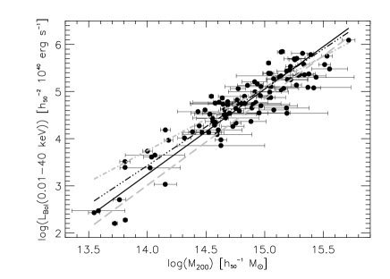
Figure 11: Gravitational mass–bolometric X-ray luminosity relation compared to predicted relations. Shown are: best fit relation for the extended sample (solid line), best fit relation determined using HIFLUGCS (triple-dot-dashed line), self-similar relation normalized by simulations of Navarro et al. (1995) (dot-dashed line), pre-heated relation given by Evrard & Henry (1991), using a normalization taken from the simulations of pre-heated clusters by Navarro et al. (1995) (dashed line).

In order to compare the empirical $L_{\rm X}$–$M_{\rm tot}$ relation with predictions a quasi bolometric luminosity, $L_{\rm Bol}$, has been calculated in the source rest frame energy range $0.01-40\,{\rm keV}$ (for the relevant range of cluster gas temperatures at least 99 % of the flux is contained in this energy range). In Fig. 11 this $L_{\rm Bol}$–$M_{200}$ relation is compared to predicted relations. The solid line shows the best fit relation for the 106 clusters in the extended sample and the triple-dot-dashed line shows the best fit relation determined using HIFLUGCS. Here the bisector fit results have been used in order to treat variables symmetrically, which is the appropriate method for a comparison to theory (e.g., Isobe et al., 1990). The dot-dashed line shows the self-similar relation ($L_{\rm Bol}\propto M^{4/3}$) normalized by the simulations of Navarro et al. (1995) and the dashed line shows the ‘pre-heated’ relation given by Evrard & Henry (1991) ($L_{\rm Bol}\propto M^{11/6}$), using a normalization taken from the simulations of pre-heated clusters by Navarro et al. (1995). The idea of pre-heating is that the intracluster gas is not cold initially, as in the self similar case, but is heated by some form of non gravitational heat input, e.g., from supernovae or AGN, before or during cluster formation. Assuming the central regions of all clusters to have the same entropy yields the latter relationship. Fig. 11 shows that measured and predicted relations are in rough agreement, the difference between the predicted relations being larger than the difference to the observed relations. Note, however, that the X-ray luminosity is one of the most uncertain quantities to be derived from simulations. Frenk et al. (1999) recently showed in a comparison of twelve different cosmological hydrodynamics codes that a factor of two uncertainty is a realistic estimate of the current accuracy. Including gas cooling in simulations worsens the situation (e.g., Balogh et al., 2001). The slopes of the observed relations are closer to the pre-heated relation. Observationally the effect of pre-heating can also result in a decrease of the gas mass fraction for low temperature systems. This has actually been observed for the clusters in our sample (Reiprich, 1998; Reiprich & Böhringer, 1999b). The possibility that winds from, e.g., supernovae – originally invoked to explain the apparent low gas content of elliptical galaxies (e.g., Mathews & Baker, 1971; Larson, 1974) – pre-heat and dilute the central gas and thereby break the self similarity has been pointed out by various authors (e.g., Kaiser 1986). Such a process would work most efficiently on the least massive clusters (e.g., White III 1991; Metzler & Evrard 1997; Ponman et al. 1999). The $L_{\rm X}$–$M_{\rm tot}$ relation and other relevant relations between physical cluster parameters of the extended sample have been discussed more thoroughly in this context in Reiprich (2001a).

One may wonder about the origin of the scatter in the $M_{\rm tot}$–$L_{\rm X}$ relation. Due to the use of pointed observations for most of the clusters and the local nature of HIFLUGCS the statistical errors of $L_{\rm X}$ are negligible. The logarithmic mean mass measurement uncertainty has been measured as 0.12. The overall scatter in log mass of the data points compared to the best fit relation is larger and has been measured as 0.21 (Tab. 12). This indicates a possible contribution of intrinsic scatter to the overall scatter in the $M_{\rm tot}$–$L_{\rm X}$ relation. An obvious candidate to cause intrinsic scatter is the central excess emission (central surface brightness exceeding single $\beta$ model surface brightness) present in a number of clusters. This excess emission may have its physical origin either in cooling flows (e.g., Fabian, 1994) or in the presence of cD galaxies (e.g., Makishima et al., 2001). A cooling flow analysis of the HIFLUGCS clusters is in progress and first results indicate that indeed clusters with a high inferred mass deposition rate lie on the high $L_{\rm X}$ side of the $M_{\rm tot}$–$L_{\rm X}$ relation (Y. Chen et al., in preparation).

In Fig. 12 the measured number of cluster member galaxies as taken from Abell et al. (1989) is compared to $L_{\rm X}$ as gravitational mass tracer. It is clearly seen that a selection by X-ray luminosity is much more efficient than a selection by Abell richness in terms of mass. Even though only the X-ray surface brightness profile and neither its normalization nor the X-ray luminosity are directly used in the X-ray mass determination via the hydrostatic equation, it is nonetheless reassuring that a similar result is obtained when $L_{\rm X}$ and richness are compared to masses estimated from optical velocity dispersions (Borgani & Guzzo, 2001).

Figure 12: Measured number of cluster member galaxies, $N_{\rm gx}$, as taken from Abell et al. (1989) and X-ray luminosity of the same (66) clusters as a function of the gravitational mass. Double clusters, whose components have been treated separately here, e.g., A3528n/s, are removed. Above the dashed line all clusters have an Abell richness $R\geq 1$.

A wide range of possible applications becomes available with the quantification of the $L_{\rm X}$–$M_{\rm tot}$ relation and its scatter. For large X-ray flux-limited cluster surveys, where individual mass determinations are currently not feasible, luminosities can be directly converted to masses. No combination of observations, simulations and theory is then needed, like the frequently used approach of relating X-ray luminosities to X-ray temperatures by an observed relation, and converting X-ray temperatures to masses using a relation where the slope is taken from theoretical arguments and the normalization from hydrodynamical simulations (e.g., Moscardini et al. 2000). The observational $L_{\rm X}$–$M_{\rm tot}$ relation has first been applied directly in this sense in the power spectral analysis of REFLEX clusters (Schuecker et al., 2001b). An example of another direct application is given in Sect. 5.3.3. The $L_{\rm X}$–$M_{\rm tot}$ relation may also be applied to convert theoretical or simulated mass functions to luminosity functions for comparison with observations of X-ray flux-limited samples, which is currently being performed in the interpretation of the REFLEX luminosity function.

At this point it is important to note that even for the highest redshift cluster in our sample ($z=0.2$) the dependence of the observational determination of $M_{\rm tot}$ and $L_{\rm X}$ on the chosen cosmological model is very weak. For instance at $z=0.2$ the increase in the luminosity distance, $D_{L}$, and the diameter distance, $D_{A}$, is less than 5 % going from ($\Omega_{\rm m}=1.0,\Omega_{\Lambda}=0$) to ($\Omega_{\rm m}=0.1,\Omega_{\Lambda}=0$). From (3) one finds that $M_{\rm tot}(<r)\propto r$ and therefore $M_{\rm tot}(<r)\propto D_{A}$, implying an increase of $M_{\rm tot}$ by less than 5 % for the two models above. For $L_{\rm X}$ one has an increase of less than 10 %. This means that the $L_{\rm X}$–$M_{\rm tot}$ relation given here can be used unchanged for various cosmological applications (unless redshift ranges are probed where evolution becomes important, in this case a model dependent redshift correction has to be introduced). A similar calculation for $V_{\rm max}$ shows that for the extreme case $z_{\rm max}=0.2$ the increase in $V_{\rm max}$ is less than 14 %, which is less than the size of the Poissonian error bars in Fig. 14.

More detailed investigations on the shape of the relation are in progress and it is also envisaged to construct a volume-limited sample, spanning a reasonably large range in luminosity and mass, to test how much the $L_{\rm X}$–$M_{\rm tot}$ relation given here is affected by being estimated partly from a flux-limited sample.

5.3 Mass Function

5.3.1 Comparison to previous estimates

Bahcall & Cen (1993) give a mass function constructed a) from optically selected clusters with masses determined from the galaxy richness and b) from the cluster X-ray temperature function given by Henry & Arnaud (1991). Very good agreement is found for masses determined within $r_{\rm A}$ between the Bahcall & Cen and HIFLUGCS mass function (Fig. 13).

Figure 13: Cumulative gravitational mass functions for HIFLUGCS using three different outer radii. Vertical error bars give the Poissonian errors. Horizontal bars indicate the individual bin sizes. Each bin contains 10 clusters, apart from the highest mass bin, which contains 13 clusters. The abundances from previous works are determined for $M_{\rm A}$.

White et al. (1993a) constrain the cluster abundance by using published values for the abundance and median velocity dispersion of richness class $R\geq 1$ Abell clusters. It is not surprising that their density is significantly higher than the HIFLUGCS density since they have intentionally used conservative mass estimates, which are overestimates of the true cluster masses.

Biviano et al. (1993) and Girardi et al. (1998) have determined the cluster mass function using optically selected cluster samples with masses determined from published line-of-sight velocity dispersions of cluster galaxies. At the completeness limit given by Girardi et al. (1998, triangle in Fig. 13) the cluster density given by Biviano et al. (1993) is about a factor of two higher than the density given by Girardi et al. (1998). The latter authors explain this by their on average 40 % smaller mass estimates due to an improved technique for removing interlopers and the use of a surface-correction term in the virial theorem. The value given by Girardi et al. itself lies significantly higher than the comparable HIFLUGCS density. The reason could lie in the fact that their optically estimated masses are in general slightly larger than the X-ray masses or that the external normalization for $R\geq 1$ ($N_{\rm gx}\geq 50$) clusters which they applied to their mass function is intrinsically higher than the normalization obtained through HIFLUGCS directly, or both. By comparing the mass estimates for a common subsample of 42 clusters it has been found that the virial masses determined by Girardi et al. (1998) are on average 25 % larger than the masses determined in this work. This difference might be smaller if masses out to the Abell radius were compared, since common radii would have been used in this case. Increasing the X-ray masses artificially by 25 %, the diamonds in Fig. 13 shift towards higher masses, but the shift is too small to account for the difference to the triangle. The large scatter in the $N_{\rm gx}$–$M_{\rm tot}$ diagram (Fig. 12) makes a reliable estimate of a best fit relation between these two quantities very difficult. Nevertheless, in order to get a rough idea of the mass within $r_{\rm A}$ that corresponds to $N_{\rm gx}=50$, we have performed fits using the minimization methods outlined earlier and find $5.1\lesssim M_{\rm A}(N_{\rm gx}=50)\lesssim 8.8\times 10^{14}\,h_{50}^{-1}\,M_{\odot}$. Note that this range is in agreement with the ranges $5$–$8\times 10^{14}\,h_{50}^{-1}\,M_{\odot}$ and $5$–$7\times 10^{14}\,h_{50}^{-1}\,M_{\odot}$ given by Bahcall & Cen (1993) and Girardi et al. (1998), respectively, for $N_{\rm gx}=50$. This mass range corresponds to a cumulative number density obtained through HIFLUGCS in the range $1.7\lesssim n(>M_{\rm A})\lesssim 8.7\times 10^{-7}\,h_{50}^{3}\,\rm Mpc^{-3}$. The external density estimate applied to normalize the Girardi et al. mass function therefore is a factor 1.2–6.2 higher than the corresponding estimate obtained here. It is therefore concluded that both effects (masses and normalization) are important but the latter factor is responsible for a larger fraction of the discrepancy. Assuming both normalizations to be determined from samples that are highly complete and representative of the local universe this may indicate that either X-ray and optical clusters are drawn from different populations or that projection effects (e.g., line of sight galaxy overdensities, which do not form a bound structure in three dimensions) possibly bias optically determined normalizations high.

Girardi & Giuricin (2000) recently extended the mass function to loose galaxy groups, finding $n(>1.8\,h_{50}^{-1}\times 10^{13}\,M_{\odot})=1.6$–$2.4\times 10^{-4}\,h_{50}^{3}\,\rm Mpc^{-3}$, which is outside the mass range we can test. They find that the group mass function can be described by a smooth extension of the cluster mass function by Girardi et al. (1998). Consistently this abundance is higher than the abundance given by Bahcall & Cen (1993) at that mass scale.

Carlberg et al. (1997) have compiled and partially reestimated abundances for local cluster samples (Henry & Arnaud, 1991; Mazure et al., 1996; White et al., 1993a; Eke et al., 1996) for comparison with higher redshift samples (the ‘$\times$’ shows the density for a sample with higher mean redshift and therefore it cannot be compared directly). Note that Borgani et al. (1999a) find that the reestimate of the mass limit of the Mazure et al. sample by Carlberg et al. (the ‘+’ at $n\approx 3\times 10^{-7}h_{50}^{3}\rm Mpc^{-3}$) may lead to an underestimated mass limit. In general the comparison to the HIFLUGCS mass function shows better agreement than the abundances given by Girardi et al. (1998) and White et al. (1993a).

The obvious importance of the definition of the cluster outer radius for the cluster mass function can be directly appreciated by noting the large differences between the mass functions determined for HIFLUGCS for $M_{500}$, $M_{200}$, and $M_{\rm A}$ in Fig. 13, especially towards lower masses. Since for self similar clusters the mass scales with the third power of the characteristic radius (Sect. 5.2), determination of the mass within a characteristic overdensity is the natural choice. We mainly give the formally determined $M_{\rm A}$ mass function for the comparison with previous mass functions and recall again that especially for the low mass systems the assumption of hydrostatic equilibrium may not be justified out to $r_{\rm A}$, and therefore our mass estimates of $M_{500}$ and $M_{200}$ should be considered much more precise than the estimates for $M_{\rm A}$.

5.3.2 Comparison to predicted mass functions

We use the standard formalism based on the Press–Schechter (PS) prescription to predict cluster mass functions for given cosmological models (see, e.g., Borgani et al. 1999b). To allow easier comparison with the theoretical literature on this subject in this paragraph $h_{100}=h_{50}/2$ is used. The mass function is then given by

$$\frac{dn(M)}{dM}=\sqrt{\frac{2}{\pi}}\,\frac{\bar{\rho}_{0}}{M}\,\frac{\delta_{\rm c}(z)}{\sigma(M)^{2}}\,\left|\frac{d\sigma(M)}{dM}\right|\exp\left(-\frac{\delta_{\rm c}(z)^{2}}{2\,\sigma(M)^{2}}\right)$$ (6)

(Press & Schechter 1974, Bond et al. 1991; see, e.g., Schuecker et al. 2001a for a compilation of published extensions of the PS mass function). Here $M$ represents the halo (cluster) virial mass and $\bar{\rho}_{0}=2.7755\times 10^{11}\,\Omega_{\rm m}\,h_{100}^{2}\,M_{\odot}\,\rm Mpc^{-3}$ is the present day mean matter density. The linear overdensity computed at present $\delta_{\rm c}(z)=\delta_{\rm c}^{\rm v}(z)\,D(0)\,D(z)^{-1}$, where the linear overdensity at the time of virialization, $\delta_{\rm c}^{\rm v}(z)$, is computed using the spherical collapse model summarized in Kitayama & Suto (1996), for $\Omega_{\rm m}=1$ using (A2) and for $\Omega_{\rm m}<1\wedge\Omega_{\rm k}=0$ using (A6,7); the linear growth factor $D(z)=2.5\,\Omega_{\rm m}\,E(z)\int_{z}^{\infty}(1+z^{\prime})\,E(z^{\prime})^{-3}\,dz^{\prime}$ and $E(z)$ has been defined in Sect. 3.2. As mentioned earlier due to the low redshift range spanned by HIFLUGCS, the effect of a redshift correction is very small and we therefore set $z=0$ for all calculations, unless noted otherwise. The variance of the cosmic mass density fluctuations

$$\sigma(M)^{2}=\sigma_{8}^{2}\frac{\int_{0}^{\infty}k^{2+n}\,T(k)^{2}\,|W(k\,R(M))|^{2}\,dk}{\int_{0}^{\infty}k^{2+n}\,T(k)^{2}\,|W(k\,8\,h_{100}^{-1}\,{\rm Mpc})|^{2}\,dk}\,,$$ (7)

where $\sigma_{8}$ represents the amplitude of density fluctuations in spheres of radius $8\,h_{100}^{-1}\,{\rm Mpc}$. Recent measurements of the cosmic microwave background (CMB) anisotropies indicate that the primordial power spectral index, $n$, has a value close to 1 (e.g., Balbi et al., 2000; Jaffe et al., 2001; Pryke et al., 2001; Wang et al., 2001; de Bernardis et al., 2001) and is therefore set to 1, unless noted otherwise. For the transfer function we use the fitting formula for Cold Dark Matter (CDM) cosmologies provided by Bardeen et al. (1986) for $q(k)=k/(\Gamma\,h_{100}\,\rm Mpc^{-1})$

$$T(k)\equiv T(q(k))=\ln(1+2.34q)/(2.34q)$$

$$\times\,[1+3.89q+(16.1q)^{2}+(5.46q)^{3}+(6.71q)^{4}]^{-1/4}\,,$$ (8)

where the shape parameter is given by (modified to account for a small normalized baryon density $\Omega_{\rm b}>0$, Sugiyama 1995)

$$\Gamma=\Omega_{\rm m}\,h_{100}\,\left(\frac{2.7\,\rm K}{T_{0}}\right)^{2}\,\exp\,\left(-\Omega_{\rm b}-\sqrt{\frac{h_{100}}{0.5}}\,\frac{\Omega_{\rm b}}{\Omega_{\rm m}}\right)\,.$$ (9)

The temperature of the CMB $T_{0}=2.726\,\rm K$ (Mather et al., 1994) and $\Omega_{\rm b}\,h_{100}^{2}=0.0193$ (Burles & Tytler, 1998), for the latter equation and (9) $h_{100}=0.71$ has been used (Mould et al., 2000). The comoving filter radius $R(M)=[3M/(4\pi\bar{\rho}_{0})]^{1/3}$ for the top hat filter function $W(x)=3\,(\sin x-x\cos x)/x^{3}$, which is adopted in this analysis, because the HIFLUGCS masses have been determined with a top hat filter, too. Since the PS recipe as outlined above assumes virial masses based on the spherical collapse model we use $M_{200}$ as approximation to the virial mass (Sect. 3.2).

Similarly to the work of Ikebe et al. (2001) the statistical uncertainty in the mass determination is incorporated in the model mass function as

$$\frac{d\tilde{n}(M)}{dM}\equiv\frac{1}{V_{\rm max}(M)}\,\int^{\infty}_{-\infty}\frac{dn(M^{\prime})}{dM^{\prime}}\,V_{\rm max}(M^{\prime})\,$$

$$\times\,(2\pi\,\bar{\sigma}_{M_{\rm tot},\log}^{2})^{-1/2}\,\exp\left(\frac{-(\log M^{\prime}-\log M)^{2}}{2\,\bar{\sigma}_{M_{\rm tot},\log}^{2}}\right)d\log M^{\prime}\,,$$ (10)

where $\bar{\sigma}_{M_{\rm tot},\log}=0.12$ represents the logarithmic mean mass measurement uncertainty. Note that since HIFLUGCS is flux-limited and not volume-limited the weighting has to be performed on the mass distribution, $N(M)/dM$, rather than on the mass function itself. The effect of this weighting on the model mass function is a slight amplitude increase at the high mass end.

For the modeling to be independent of the precise knowledge of the $L_{\rm X}$–$M_{\rm tot}$ relation the quantitative comparison has been performed using a standard $\chi^{2}$ procedure on the differential binned mass function given in Fig. 14 (rather than using a maximum likelihood approach on the mass distribution). After identifying the crude position where $\chi^{2}$ is minimal in a large $\Omega_{\rm m}$–$\sigma_{8}$ parameter space region the $\chi^{2}$ values have been calculated in a fine grid of 200 by 200 $\Omega_{\rm m}$–$\sigma_{8}$ values in the range $0.05\leq\Omega_{\rm m}\leq 0.26$ and $0.65\leq\sigma_{8}\leq 1.30$. A flat cosmic geometry has been assumed, i.e. $\Omega_{\rm m}+\Omega_{\Lambda}=1$. The cosmological constant enters the calculation only through $\delta_{\rm c}$, however, and therefore has a negligible influence here. The minimum and statistical error ellipses for some standard confidence levels (c.l.) are given in Fig. 15. The tight constraints obtained show that with HIFLUGCS we can go beyond determining an $\Omega_{\rm m}$–$\sigma_{8}$ relation and put limits on $\Omega_{\rm m}$ and $\sigma_{8}$ individually. It is found that

$$\Omega_{\rm m}=0.12^{+0.06}_{-0.04}\quad{\rm and}\quad\sigma_{8}=0.96^{+0.15}_{-0.12}$$ (11)

(90 % c.l. statistical uncertainty for two interesting parameters), indicating a relatively low value for the density parameter. The large covered mass range, the specific region in $\Omega_{\rm m}$–$\sigma_{8}$ parameter space, and the assumption of CDM cosmological models with given $H_{0}$, $\Omega_{\rm b}$, $n$, and $T_{0}$ allow to derive these tight constraints from a local cluster sample. For comparison for a given $\sigma_{8}$ value the $\Omega_{\rm m}$ value which minimizes $\chi^{2}$ is calculated. In the interval shown in Fig. 15 these pairs can then roughly be described by a straight line in log space given by

$$\sigma_{8}=0.43\,\Omega_{\rm m}^{-0.38}\,.$$ (12)

In Fig. 14 we also plot the best fit model mass functions for given $\Omega_{\rm m}=0.5$ and $\Omega_{\rm m}=1.0$ and one notes immediately that these value pairs give a poorer description of the shape of the mass function. The slight differences between the best fit values for $\sigma_{8}$ and the ones expected from (12) are caused by the fact that the simple power law is only an approximation to the real shape of the error ellipse and weakly by the extrapolation involved. Previous estimates have generally yielded a combination of slightly higher $\Omega_{\rm m}$–$\sigma_{8}$ values (e.g., Peacock 1999, Sect. 17.2). It has to be noted, however, that for instance in the important work of White et al. (1993a), who find $\sigma_{8}\approx 0.57\,\Omega_{\rm m}^{-0.56}$, the authors explicitly state that their estimates of $\sigma_{8}$ are probably biased high due to their conservative mass estimates.

Figure 14: HIFLUGCS mass function compared to the best fit model mass function with $\Omega_{\rm m}=0.12$ and $\sigma_{8}=0.96$ (solid line). Also shown are the best fit model mass functions for fixed $\Omega_{\rm m}=0.5$ ($\Rightarrow\sigma_{8}=0.60$, dashed line) and $\Omega_{\rm m}=1.0$ ($\Rightarrow\sigma_{8}=0.46$, dotted line).

Before exploring sources of systematic errors let us evaluate our treatment of the shape parameter $\Gamma$. By applying the Bardeen et al. (1986) fitting formula to calculate the transfer function we have adopted the assumption of a CDM universe, i.e. $\Omega_{\rm m}-\Omega_{\rm b}=\Omega_{\rm CDM}$. Within this model $\Gamma$ and $\Omega_{\rm m}$ are not independent. For a small $\Omega_{\rm b}/\Omega_{\rm m}$ ratio $\Gamma$ is given by (9). However, to test its influence we have set $\Gamma$ to a fixed value of 0.19 as implied by Large Scale Structure (LSS) measurements of galaxies and clusters (e.g., Szalay et al., 2001; Schuecker et al., 2001b, see also the discussion at the end of this Section). The best fit values for $\Omega_{\rm m}$ and $\sigma_{8}$ change significantly, the $\Omega_{\rm m}$ value becoming smaller and the $\sigma_{8}$ value larger. The $\Omega_{\rm m}$–$\sigma_{8}$ relation changes slightly to about $\sigma_{8}=0.40\,\Omega_{\rm m}^{-0.46}$ for the $\Omega_{\rm m}$ range [0.04–0.30] (note that for this range relation (12) translates to about $\sigma_{8}=0.39\,\Omega_{\rm m}^{-0.43}$, the steepening being mainly due to a strong increase of $\sigma_{8}$ for the very lowest $\Omega_{\rm m}$ values). The error ellipse in general becomes much longer when $\Gamma$ is set to a fixed value, preventing the possibility to obtain tight individual constraints on $\Omega_{\rm m}$ and $\sigma_{8}$, even though $\Omega_{\rm m}=1.0$ is still excluded at least at the 90 % c.l. for all $\Gamma\geq 0.03$. The decreased sensitivity is due to the loss of the amplification of a change of $\Omega_{\rm m}$ through $\Gamma$ (to first order $\Omega_{\rm m}\propto\Gamma$, eq. 9), since both a larger (smaller) $\Omega_{\rm m}$ and a larger (smaller) $\Gamma$ result in steeper (less steep) model mass functions. Having found a dependence of the results on $\Gamma$ we tried to constrain $\Gamma$ directly from the observations, as done by previous authors (e.g., Borgani et al., 1999b). We have set $\Gamma$ to 31 different fixed values in the range $0.01\leq\Gamma\leq 0.50$ and calculated a $\chi^{2}_{\rm min}$ for each of those by varying $\Omega_{\rm m}$ and $\sigma_{8}$. The result is shown in Fig. 16. The conclusion is that the data do not contain enough information to provide an independent constraint on $\Gamma$. Therefore we have taken advantage of the dependence of $\Gamma$ on $\Omega_{\rm m}$ within the CDM framework and have continued to calculate $\Gamma$ with eq. 9. Notice that this procedure requires additional knowledge about $H_{0}$ and $\Omega_{\rm b}$. The influence of the uncertainty of these two parameters is tested along with various other possible systematic uncertainties in the following. It is important to note that the best fit value for $\Omega_{\rm m}$ is not determined solely through (9) but also directly through $\bar{\rho}_{0}$ in (6) and through the filter radius $R(M)$.

The quoted error ranges have been calculated from the $\chi^{2}$ procedure. Most of the remaining part of this Section is devoted to an identification and quantification of possible systematic uncertainties. The quantitative results are summarized in Tab. 5.3.2.

Due to the large given ranges of several orders of magnitude in mass and especially density the $\chi^{2}$ values have been determined from comparison model/data naturally in log space. However, we have verified that the same calculation in linear space yields best fit values lying within the 68 % error ellipse.

In Sect. 4.2 arguments have been given why we have used $V_{\rm max}(L_{\rm X})$ for the determination of the mass function. Nevertheless if $V_{\rm max}(M_{\rm tot})$ is used instead (see Fig. 7), consistent results are obtained. Since in this case we want to estimate $L$ from $M$ the relation ($L\mid M$) is the appropriate one (e.g., Isobe et al., 1990). Performing a fit to a mass function constructed with $V_{\rm max}(M_{\rm tot})$ results in best fit values $\Omega_{\rm m}=0.14$ and $\sigma_{8}=0.86$, which is consistent with the error range given in (11).

The data point in Fig. 14 that may be affected most by cosmic variance is the one at the lowest mass, since the maximum search volume is smallest for the clusters in this bin. We therefore tested the sensitivity of the best fit results on this last point by ignoring it. The decrease in the covered mass range of course increases the resulting error ellipse, but the best fit values vary only within the (smaller) 68 % error ellipse. It may be worth noting that leaving out the highest mass bin or leaving out the highest and lowest mass bin changes the best fit values only within the 90 % error ellipse.

Simulations seem to indicate that the mass density profile of virialized halos follows the NFW profile (Navarro et al., 1996, 1997, but see, e.g., Kravtsov et al. 1998). As test therefore gravitational masses have been recalculated assuming the dark matter density to follow an NFW profile based on the measured values for $\beta$ and $r_{\rm c}$. The approximation $r_{\rm s}=r_{\rm c}/0.22$ and $b=\beta/0.9$ given by Makino et al. (1998) has been used combined with their eqs. 7 and 9. $r_{200}$ and $M_{200}$ have been redetermined based on this model and the resulting mass function has been compared to model mass functions. On average it is found that the NFW masses are a factor of 0.90 lower, the difference being smaller for high mass clusters than for low mass ones. The values for $\Omega_{\rm m}$ and $\sigma_{8}$ for which $\chi^{2}$ is minimal lie within the 90 % statistical error ellipse shown in Fig. 15. Therefore the choice of mass calculation does not affect the results significantly.

As shown in Sect. 3.2 it is possible that the assumption of isothermality leads to an overestimate of the cluster masses on average. Therefore the robustness of the results has been tested by multiplying the isothermal cluster masses by 0.80 and recalculating the minimum. As expected values for both $\Omega_{\rm m}$ and $\sigma_{8}$ are found to be lower. But the new minimum is contained well within the error ranges given in (11). On the other hand in Sect. 5.3.1 it has been shown by comparison with optical virial mass measurements that masses could possibly be underestimated. After increasing all cluster masses by 25 % a fit shows that both $\Omega_{\rm m}$ and $\sigma_{8}$ become slightly larger, but again they lie well within the range (11). Therefore these tests indicate that the constraints obtained here are fairly insensitive against systematic uncertainties in the mass measurements. Note that systematic effects that show a mass dependence have a higher potential to affect the individual best fit values of $\Omega_{\rm m}$ and $\sigma_{8}$ than effects which simply shift all data points by about the same amount in the same direction. However, no indications for a mass dependence of the differences between the above mass estimations have been found.

Figure 15: Statistical confidence contours for the $\chi^{2}$ procedure. The cross indicates the position of the minimum, $\chi^{2}_{\rm min}$. Ellipses indicate the 68 %, 90 %, 95 %, and 99 % confidence levels for two interesting parameters, i.e. $\Delta\chi^{2}\equiv\chi^{2}-\chi^{2}_{\rm min}=$ 2.30, 4.61, 6.17, and 9.21, respectively.

It has been mentioned that masses calculated within $r_{500}$ are less affected by systematic uncertainties because less extrapolation beyond $r_{\rm X}$ is needed and because according to simulations the assumption of hydrostatic equilibrium can be more safely applied. Nevertheless we have used $M_{200}$ for the comparison to predicted mass functions because it is a better approximation to the cluster virial mass. However, for comparison the best fit values have also been determined using $M_{500}$, knowing that virial masses are probably underestimated this way. The result is that the best fit value for $\Omega_{\rm m}$ changes only marginally. The best fit $\sigma_{8}$ value is slightly lower than allowed by the statistical error. On the other hand the spherical collapse model implies that one may need to extrapolate even further than $r_{200}$ for low density universes. For instance in a flat universe $\Omega_{\rm m}=0.2$ implies that the virial radius is close to $r_{87}$. Therefore a mass function has been constructed using $M_{87}$ as cluster masses, knowing that these masses are likely to be rather uncertain. Nevertheless the resulting best fit $\Omega_{\rm m}$ value again varies only insignificantly whereas the $\sigma_{8}$ value becomes significantly larger. Note that for both tests the best fit value for $\Omega_{\rm m}$ hardly changes.

As mentioned in Sect. 3.2 it has been shown that the small range of low redshifts covered here ensures that no redshift corrections need to be applied. Nevertheless we have tested whether or not the best fit parameter values change if $M_{200}$ is calculated using $\rho_{\rm c}=\rho_{\rm c}(z)$ for the extreme (strong evolution) case ($\Omega_{\rm m}=1,\Omega_{\Lambda}=0$), i.e., $\rho_{\rm c}=4.6975\times 10^{-30}\,(z+1)^{3}\,\rm g\,cm^{-3}$ for each cluster redshift. The model mass function is then calculated for the mean redshift of HIFLUGCS, $\langle z\rangle=0.05$, using the formulae outlined in the beginning of this Section. We have found that within our grid the best fit values do not change at all and also the error ellipses are almost not affected, thereby confirming that the application of redshift corrections does not affect the results.

Figure 16: Minimal $\chi^{2}$ values calculated by varying $\Omega_{\rm m}$ and $\sigma_{8}$ for a variety of fixed values of $\Gamma$ instead of using eq. 9. The dashed line represents the 68 % c.l. statistical uncertainty for one interesting parameter. This line actually underestimates the uncertainty since the procedure involves three interesting parameters. Obviously $\Gamma$ cannot be constrained significantly.

The value $H_{0}=71\,\rm km\,s^{-1}\,Mpc^{-1}$ has been adopted for the calculation of model mass functions based on the recent combination of constraints obtained using the Hubble Space Telescope (Mould et al., 2000). Setting the Hubble constant to their lower limit, $H_{0}=65\,\rm km\,s^{-1}\,Mpc^{-1}$, does not affect the best fit parameter values significantly. Using even $H_{0}=60\,\rm km\,s^{-1}\,Mpc^{-1}$ changes the results for $\Omega_{\rm m}$ and $\sigma_{8}$ only well within the 68 % error ellipse. In Tab. 5.3.2 results have also been listed for $H_{0}=50$ and $80\,\rm km\,s^{-1}\,Mpc^{-1}$ showing that even variations within this range change the $\Omega_{\rm m}$ and $\sigma_{8}$ values only within their statistical uncertainties given in (11). Therefore our constraints on these cosmological parameters do not depend significantly on the specific choice of $H_{0}$.

A baryon density based on measurements of the primordial deuterium to hydrogen ratio combined with standard nucleosynthesis theory has been used in this work. The used value also agrees with recent CMB measurements (e.g., Pryke et al., 2001). However, we have also calculated the minimum for the values $\Omega_{\rm b}\,h_{100}^{2}=0.0100$ and $0.0300$ finding that the position of the minimum in each case does not deviate significantly from our original result.

The primordial power spectral index has been set to $n=1$ based on measurements of the CMB fluctuations. The influence of a change in this parameter has been estimated by calculating the minimum for the values $n=0.8$ and $n=1.2$. The differences in the best fit parameters are smaller than the statistical uncertainties given in (11).

Since we have found that for the estimate of the statistical errors we need to explore ranges $\Omega_{\rm m}<0.1$ for $\Omega_{\rm b}\sim 0.04$ we regarded it necessary to check if the approximation to the transfer function as given in the beginning of this Section is still applicable. Recently Eisenstein & Hu (1998) derived a fitting function, that includes, e.g., also the oscillations induced by the baryons, which gives a better description of transfer functions computed with CMBFAST (Seljak & Zaldarriaga, 1996) than fitting functions for zero or small baryon contribution to the total matter density derived previously. Therefore we incorporated this improved version of an analytic transfer function in the $\chi^{2}$ procedure. We have found that within our grid there is only a very weak shift of the minimum, the choice of the Bardeen et al. (1986) fitting function combined with the shape parameter given by Sugiyama (1995) therefore seems to be accurate enough for our purposes. However, the confidence contours towards low $\Omega_{\rm m}$ are getting compressed when the Eisenstein & Hu (1998) fitting function is used, thereby slightly decreasing the area of the error ellipse for a given confidence level. Since we regard the latter statistical error ellipse as more realistic, we show this one in Fig. 15.

Table 5: Systematic uncertainties

$\Omega_{\rm m}$	$\sigma_{8}$	$\Delta\Omega_{\rm m}$	$\Delta\sigma_{8}$	Test
0.116	0.928	$\pm 0.000$	$-0.026$	(1)
0.137	0.865	$+0.021$	$-0.094$	(2)
0.150	0.897	$+0.034$	$-0.062$	(3)
0.092	1.082	$-0.024$	$+0.124$	(4)
0.083	1.050	$-0.034$	$+0.091$	(5)
0.150	0.860	$+0.034$	$-0.099$	(6)
0.107	0.907	$-0.009$	$-0.052$	(7)
0.132	1.004	$+0.016$	$+0.046$	(8)
0.106	0.826	$-0.011$	$-0.133$	(9)
0.108	1.242	$-0.008$	$+0.281$	(10)
0.116	0.959	$\pm 0.000$	$\pm 0.000$	(11)
0.118	0.956	$+0.002$	$-0.003$	(12)
0.153	0.861	$+0.037$	$-0.098$	(13)
0.108	0.991	$-0.008$	$+0.033$	(14)
0.106	1.001	$-0.011$	$+0.042$	(15)
0.128	0.923	$+0.012$	$-0.036$	(16)
0.148	0.874	$+0.032$	$-0.085$	(17)
0.094	1.056	$-0.022$	$+0.098$	(18)

Note. — See text for a more detailed description of the tests. The differences to the best fit results have been been calculated with more digits than given here.

References. — (1) $\chi^{2}$ calculated in linear space. (2) $V_{\rm max}(M_{\rm tot})$ used with relation ($L\mid M$) for HIFLUGCS (Tab. 8). (3) Lowest mass bin ignored. (4) Highest mass bin ignored. (5) $r_{200}$ and $M_{200}$ calculated assuming NFW profile. (6) Universal mass function. (7) $M_{200}$ reduced by factor 0.80. (8) $M_{200}$ increased by factor 1.25. (9) $M_{500}$ used. (10) $M_{87}$ used. (11) Redshift correction applied for cluster mass determination and model mass function calculation. (12) Transfer function calculated using Eisenstein & Hu fitting formula. (13) $h_{100}$ set to 0.5. (14) $h_{100}$ set to 0.8. (15) $\Omega_{\rm b}$ set to 0.0100 $h_{100}^{-2}$. (16) $\Omega_{\rm b}$ set to 0.0300 $h_{100}^{-2}$. (17) $n$ set to 0.8. (18) $n$ set to 1.2.

We have also tested whether or not the recently found deviations of the PS formalism compared to large $N$-body simulations (e.g., Governato et al., 1999; Jenkins et al., 2001) have a significant influence on the results obtained here. We have compared the best fit PS model ($\Omega_{\rm m}=0.12$, $\sigma_{8}=0.96$) to the model obtained using the ‘universal’ mass function (fit to $N$-body simulations, Jenkins et al. 2001) for the same parameter values. These two models agree well for $M\lesssim 10^{15}\,h_{50}^{-1}\,M_{\odot}$. The differences become larger than the size of the Poissonian error bars (Fig. 14) for $M\gtrsim 2\times 10^{15}\,h_{50}^{-1}\,M_{\odot}$, in the sense that the Jenkins et al. mass function predicts higher cluster abundances than PS. For larger values of $\Omega_{\rm m}$ the differences become comparable to the size of the error bars at lower masses, e.g., for $\Omega_{\rm m}=\sigma_{8}=0.5$ around $M\sim 5\times 10^{14}\,h_{50}^{-1}\,M_{\odot}$. To estimate the influence of these differences on the best fit values derived using the PS mass function, we adjusted the parameter values of the Jenkins et al. model to reproduce the PS mass function, finding $\Omega_{\rm m}=0.15$ and $\sigma_{8}=0.86$. The value for $\Omega_{\rm m}$ becomes slightly larger but the combination of both values is still contained within the 90 % error ellipse. We therefore conclude that the differences between the model mass functions do not significantly affect the interpretation of the HIFLUGCS mass function. Moreover we regard this test as confirmation of the validity of the PS mass function for the accuracy needed here.

Almost all identified systematics give rise to smaller uncertainties than the statistical uncertainties (eq. 11). However, it is not impossible that several systematics combined have a significant effect. In order to determine the highest $\Omega_{\rm m}$ value allowed by a conspiracy of all identified uncertainties, all positive $\Delta\Omega_{\rm m}$ values from Tab. 5.3.2 have been added to the positive statistical uncertainty for $\Omega_{\rm m}$ and this sum has been added to the $\Omega_{\rm m}$ value which minimizes $\chi^{2}$ ($\Omega_{\rm m}=0.12$). In this worst case procedure the upper limit

$$\Omega_{\rm m}<0.31$$ (13)

has been found.

Using $\Omega_{\rm b}=0.19\pm 0.08\,h_{50}^{-3/2}\,\Omega_{\rm m}$, as derived from the mean gas mass fraction within $r_{200}$ for the 106 clusters in the enlarged sample, results in model mass functions very similar to the ones calculated using the baryon fraction given by Burles & Tytler (1998). It is therefore not surprising that the best fit values for $\Omega_{\rm m}$ and $\sigma_{8}$ vary only well within the 68 % error ellipse if the former $\Omega_{\rm b}$ determination is used. Moreover it is worth noting that combining these two measurements of $\Omega_{\rm b}$ gives further evidence for a low value for $\Omega_{\rm m}$ by yielding an estimate $\Omega_{\rm m}=0.34^{+0.22}_{-0.10}$ using $H_{0}=71\,\rm km\,s^{-1}\,Mpc^{-1}$ (Mould et al., 2000), where the error has been determined from the standard deviation of $\Omega_{\rm b}$ given above. This value for $\Omega_{\rm m}$ is an upper limit since baryons, e.g., contained in the cluster galaxies or forming part of the dark matter have been neglected. A low value for $\Omega_{\rm m}$ has been indicated by this method for smaller cluster samples by several works previously (e.g., White & Frenk 1991; Briel et al. 1992; Böhringer 1993; White et al. 1993b; White & Fabian 1995; Ettori & Fabian 1999; but see Sadat & Blanchard 2001). One has to keep in mind, however, that this estimate extrapolates the gas fraction from cluster scale to cosmic scales. For the clusters in our sample we have found that the gas fraction is not constant but varies with radius and cluster mass (Reiprich & Böhringer, 1999b), therefore further observational tests of this assumption may be useful.

Table 6: Examples of previous results for given $\Omega_{\rm m}$

$\Omega_{\rm m}$	$\sigma_{8}$	Relation	Ref.
0.30	1.12	$\sigma_{8}=0.57\,\Omega_{\rm m}^{-0.56}$	1
0.30	1.16	$\sigma_{8}=0.60\,\Omega_{\rm m}^{-0.59+0.16\Omega_{\rm m}-0.06\Omega_{\rm m}^{2}}$	2
0.30	0.93	$\sigma_{8}=0.52\,\Omega_{\rm m}^{-0.52+0.13\Omega_{\rm m}}$	3
0.30	1.01	$\sigma_{8}=0.60\,\Omega_{\rm m}^{-0.46+0.09\Omega_{\rm m}}$	4
0.30	0.78		5
0.30	0.99	$\sigma_{8}=0.56\,\Omega_{\rm m}^{-0.47}$	6
0.30	0.96	$\sigma_{8}=0.58\,\Omega_{\rm m}^{-0.47+0.16\Omega_{\rm m}}$	7
0.30	0.96		8
0.30	1.02	$\sigma_{8}=0.495\,\Omega_{\rm m}^{-0.60}$	9
0.30	0.91	$\sigma_{8}=0.59\,\Omega_{\rm m}^{-0.57+1.45\Omega_{\rm m}-3.48\Omega_{\rm m}^{2}+3.77\Omega_{\rm m}^{3}-1.49\Omega_{\rm m}^{4}}$	10
0.30	0.68	$\sigma_{8}=0.43\,\Omega_{\rm m}^{-0.38}$	11

References. — (1) White et al. 1993a. (2) Viana & Liddle 1996. (3) Eke et al. 1996. (4) Girardi et al. 1998. (5) Markevitch 1998. (6) Viana & Liddle 1999. (7) Borgani et al. 1999b. (8) Blanchard et al. 2000. (9) Pierpaoli et al. 2001. (10) Oukbir & Arnaud 2001. (11) This work.

Let us briefly discuss the role of $\Gamma$ again. The constraints (11) together with $h_{100}=0.71$, $\Omega_{\rm b}\,h_{100}^{2}=0.0193$, and eq. 9 imply $\Gamma=0.06^{+0.04}_{-0.05}$, which is significantly lower than values for $\Gamma$ determined through LSS studies of galaxies (e.g., Szalay et al. 2001 have found $\Gamma=0.188\pm 0.04$) or clusters (e.g., Schuecker et al. 2001b have found $\Gamma=0.195\pm 0.055$). Adopting the worst case upper limit on $\Omega_{\rm m}$ found above yields an upper limit $\Gamma<0.18$ consistent with the LSS results. However, also many previous studies of cluster abundances have yielded low values for $\Gamma$. For instance Eke et al. (1998) have found $\Gamma\approx 0.09\pm 0.08$; Henry (2000) has found $\Gamma\approx 0.05\pm 0.22$; Oukbir & Arnaud (2001) have found $\Gamma=0.05\,\Omega_{\rm m}^{-0.71+0.89\,\Omega_{\rm m}}$ which, e.g., for $\Omega_{\rm m}=0.3$ yields $\Gamma\approx 0.09$; judging from their Fig. 3 and their best fit values for a spatially flat universe Borgani et al. (2001) have found $\Gamma\approx 0.1$, however, not significantly constrained. It is unclear whether these values indicate a significant discrepancy but it is interesting to note that cluster abundances seem to favor lower values for $\Gamma$ than LSS studies do. If significant this could possibly imply either unidentified systematic errors in one or both measurements – from the cluster abundance side one could for instance imagine a higher merger rate for more massive clusters resulting in overestimated X-ray luminosities, temperatures, and masses for the massive clusters resulting in less steep $L_{\rm X}$, $T_{\rm X}$, and $M_{\rm tot}$ functions and therefore in a decreased value for $\Gamma$ (and possibly $\Omega_{\rm m}$) – or that the description of the power spectrum using a single $\Gamma$ parameter on all scales is not accurate (e.g., Eisenstein & Hu 1998; Saslaw 2000, Sect. 33.3.3).

Even though we made a conservative estimate by neglecting the possible presence of gas temperature gradients, previous estimates obtained from cluster abundances generally yielded higher values for $\Omega_{\rm m}$ and $\sigma_{8}$ (e.g., White et al., 1993a; Girardi et al., 1998). For the latter two works one could have expected this already from Fig. 13 and possible reasons have been discussed in Sect. 5.3.1. Recently a number of constraints on $\Omega_{\rm m}$ and $\sigma_{8}$ have been obtained using different kinds of distribution functions assuming relations between the measured quantities and mass. Some of them incorporated additional dynamical information from the evolution of the corresponding distribution function. Especially intracluster gas temperature functions have been constructed and used frequently. In Tab. 5.3.2 some results, which allowed a simple comparison for a given $\Omega_{\rm m}=0.3$, are listed. If there was a choice, results assuming flat cosmological models and isothermal clusters are quoted. This Table is not a complete summary of recent results but merely shows that previous results yielded higher values for $\sigma_{8}$ than obtained here from a newly constructed sample (even using $M_{87}$ instead of $M_{200}$ would increase the $\sigma_{8}$ value only up to 0.82). The reasons may be manifold. Some have been discussed above. Other reasons may include different sources of temperature estimates. For instance Pierpaoli et al. (2001) used cooling flow corrected temperatures given by White (2000), which are generally higher than temperatures derived previously. Using theoretical/simulated $M_{\rm tot}$–$T_{\rm gas}$ relations (e.g., Evrard et al., 1996; Bryan & Norman, 1998) to connect observed temperature functions with theoretical mass functions will on average also result in higher values for $\sigma_{8}$, since these relations have been shown to have higher normalizations than observed X-ray mass–temperature relations (e.g., Horner et al., 1999; Nevalainen et al., 2000; Finoguenov et al., 2001). Assuming low temperature groups to be affected by non gravitational heat input, temperature functions, unlike X-ray mass functions which incorporate the additional information of the gas density profile, would show an additional artificial increase towards low temperatures. If not taken into account, e.g., by use of a modified $M_{\rm tot}$–$T_{\rm gas}$ relation, this effect would result in artificially increased values for $\Omega_{\rm m}$ (see Fig. 14). Also the completeness and representativeness of the used cluster samples obviously play an important role for the $\Omega_{\rm m}$–$\sigma_{8}$ determination. Here advantage has been taken of the currently best available local sample in the sense of homogeneous X-ray selection, completeness, size, and availability of high quality observations. The results obtained here are, however, in good agreement with the results from the power spectral analysis of the 452 REFLEX clusters. Schuecker et al. (2001b) find for a given $\Lambda$CDM model ($\Omega_{\rm m}=0.3$) that $\sigma_{8}=0.7$ represents the data well, which is very close to $\sigma_{8}=0.68$ expected using relation (12) found here. Moreover the (1-$\sigma$) range $0.17\leq\Omega_{\rm m}\leq 0.37$ (using $h=0.71$ in their eq. 18) quoted for $\Omega_{\rm m}$ directly is also consistent with the 90 % range determined here. Furthermore Ikebe et al. (2001), who analyzed the HIFLUGCS temperature function using temperatures from homogeneously reanalyzed ASCA data, find $\Omega_{\rm m}=0.18_{-0.05}^{+0.08}$ and $\sigma_{8}=0.96_{-0.09}^{+0.11}$ (90 % c.l. statistical uncertainty; assuming an open cosmology) by comparison with Press–Schechter models, which is in good agreement with our results. Moreover, after this paper had been submitted another paper appeared on astro-ph (Borgani et al., 2001), where the authors also find $\Omega_{\rm m}$–$\sigma_{8}$ values that agree with values calculated using relation (12) presented here.

5.3.3 Mass function estimated using $L_{\rm X}$–$M_{\rm tot}$ relation

To show consistency and the power of the $L_{\rm X}$–$M_{\rm tot}$ relation, we have also performed fits to ‘mass’ functions, where masses have been estimated from the measured X-ray luminosity. Relations for the flux-limited sample have been used to get the best mass estimate for the cluster luminosities included in HIFLUGCS. Mass functions for the two extreme relations ($M\mid L$) with $\alpha=1.538$ and ($L\mid M$) with $\alpha=1.310$ are shown in Fig. 17. First of all one notes the fairly good agreement between the three mass functions. In detail the differences between the two mass functions estimated from different luminosity–mass relations can be understood by considering that at the low luminosity end the steeper relation predicts a higher mass for a given luminosity than the shallower relation, resulting in a shift towards higher masses of the mass function. At the high mass side the effect is opposite, resulting in a shift towards lower masses for the steeper relation. On average the points for the steeper relation lie higher which is caused by the fact that a steeper relation results in a smaller $dM$ on average, which gives rise to an increased $dn/dM$. The differences to the mass function calculated using the measured masses are again understood by a similar comparison and are partially caused by a possible deviation of the shape of the $L_{\rm X}$–$M_{\rm tot}$ relation from a pure power law. Despite these small differences performing an actual fit results in the ($\Omega_{\rm m}$, $\sigma_{8}$) values (0.14, 0.85) for ($L\mid M$) and (0.22, 0.74) for ($M\mid L$). The first case is consistent with the error range given in (11) and in the second case the 90 % statistical error ellipse overlaps with the 90 % ellipse in Fig. 15. From the above and Fig. 14 it is clear that using steeper luminosity–mass relations results in higher values for $\Omega_{\rm m}$ and lower values for $\sigma_{8}$. Here we want to estimate $M$ from $L$ and therefore ($M\mid L$) is the appropriate relation to use. This test shows that with a comparatively easy to obtain X-ray luminosity function of a statistical cluster sample and with the knowledge of the empirical $L_{\rm X}$–$M_{\rm tot}$ relation (even if approximated as simple power law) and its scatter as presented here useful constraints on cosmological parameters can be set by construction of a ‘quasi mass function’.

Figure 17: HIFLUGCS mass function (filled circles) compared to ‘mass’ functions estimated using measured luminosities and luminosity–mass relations (open symbols). Squares have been calculated using the ($M\mid L$) relation and triangles using the ($L\mid M$) relation for HIFLUGCS clusters.

5.4 Total Gravitating Mass in Clusters

To estimate the fraction of the gravitational mass density relative to the critical density contained in galaxy clusters, $\Omega_{\rm Cluster}(>M_{\rm tot,min})=1/\rho_{\rm c}\int_{M_{\rm tot,min}}^{\infty}M_{\rm tot}\,\phi(M_{\rm tot})\,dM_{\rm tot}$, the individual cluster masses divided by the corresponding maximum search volumes have been summed up for HIFLUGCS, i.e., $\Omega_{\rm Cluster}=1/\rho_{\rm c}\sum_{i}M_{200,i}/V_{{\rm max},i}$. Note that the determination of $\Omega_{\rm Cluster}$ is independent of the Hubble constant. The cumulative diagram for $\Omega_{\rm Cluster}(>M_{200})$ is shown in Fig. 18. In order to perform a conservative error estimate, HIFLUGCS has been split into two parts with $b_{\rm II}\geq+20\,\rm deg$ and $b_{\rm II}\leq-20\,\rm deg$, and the results for these subsamples are also shown in the Figure. This estimate is conservative because HIFLUGCS is about twice as large as each subsample. Taking the second and third lowest mass clusters together with the maximum mass range given by their individual uncertainties, we obtain

$$\Omega_{\rm Cluster}=0.012^{+0.003}_{-0.004}$$ (14)

for masses larger than $6.4^{+0.7}_{-0.6}\times 10^{13}\,h_{50}^{-1}\,M_{\odot}$, i.e., the total gravitating mass contained within the virial radius of clusters amounts only to $1.2^{+0.3}_{-0.4}$ percent of the total mass in a critical density universe. Combined with our best estimate $\Omega_{\rm m}=0.12$ this implies that about 90 % of the total mass in the universe resides outside virialized cluster regions above the given minimum mass. If galaxies trace mass it also follows that by far most of the galaxies do not sit in clusters. This result is consistent with the general presumption that clusters are rare objects, rare peaks in the density distribution field.

Figure 18: Mass density contained in galaxy clusters as a function of minimum mass. Filled circles indicate the complete HIFLUGCS, open triangles indicate the 34 clusters north of the galactic plane, and open diamonds the 29 clusters at southern galactic latitudes included in HIFLUGCS.

Comparing the diagram to the mass fraction $\Omega_{\rm Cluster}=0.028^{+0.009}_{-0.008}$ in clusters with masses larger than $2\times 10^{14}\,h_{50}^{-1}\,M_{\odot}$ given by Fukugita et al. (1998), based on the mass function determined by Bahcall & Cen (1993), one finds that their estimate is a factor 4–5 higher. However, the Bahcall & Cen mass function is given for $M_{\rm A}$ and we get a consistent result if we calculate $\Omega_{\rm Cluster}$ using our formally determined cluster masses within $r_{\rm A}$. It needs to be pointed out that at $M_{\rm A}\sim 2\times 10^{14}\,h_{50}^{-1}\,M_{\odot}$ we find that the typical virial radius is $\sim 1\,h_{50}^{-1}\,{\rm Mpc}$ and a mass determination at $3\,h_{50}^{-1}\,{\rm Mpc}$ based on the assumption of virial equilibrium may therefore be rather uncertain and possibly leading to overestimates of $\Omega_{\rm Cluster}$. This becomes more crucial if mass functions for $M_{\rm A}$ are extrapolated even down to galaxy masses. This way Fukugita et al. (1998) find $\Omega_{\rm Group}=0.12\pm 0.02$ within the mass range $2\times 10^{12}$–$2\times 10^{14}\,h_{50}^{-1}\,M_{\odot}$, which, compared to our results from the previous Section, would account already for almost all mass in the universe.

6 Summary

An X-ray selected and X-ray flux-limited sample comprising the 63 X-ray brightest galaxy clusters in the sky (excluding the galactic band, called HIFLUGCS) has been constructed based on the ROSAT All-Sky Survey. The flux limit has been set at $2\,\times 10^{-11}\,{\rm ergs\,s^{-1}\,cm^{-2}}$ in the energy band $0.1-2.4\,{\rm keV}$. It has been shown that a high completeness is indicated by several tests. Due to the high flux limit this sample can be used for a variety of applications requiring a statistical cluster sample without any corrections to the effective survey volume.

Mainly high quality pointed observations have been used to determine fluxes and physical cluster parameters. It has been shown that a tight correlation exists between the X-ray luminosity and the gravitational mass using HIFLUGCS and an extended sample of 106 galaxy clusters. The relation and its scatter have been quantified using different fitting methods. A comparison to theoretical and numerical predictions shows an overall agreement. This relation may be directly applied in large X-ray cluster surveys or dark matter simulations for conversions between X-ray luminosity and gravitating mass.

Using HIFLUGCS the gravitational mass function has been determined for the mass interval $3.5\times 10^{13}<M_{200}<5.2\times 10^{15}\,h_{50}^{-1}\,M_{\odot}$. Comparison with Press–Schechter mass functions assuming CDM power spectra has yielded tight constraints on cosmological parameters. The large covered mass range has allowed to put constraints on relevant parameters individually. Specifically we have found $\Omega_{\rm m}=0.12^{+0.06}_{-0.04}$ and $\sigma_{8}=0.96^{+0.15}_{-0.12}$ (90 % c.l. statistical uncertainty). Various tests for systematic uncertainties have been performed, including comparison of the Press–Schechter mass function with the most recent results from large $N$-body simulations, almost always yielding uncertainties smaller than the statistical uncertainties. Combining all identified systematic uncertainties in a worst case scenario results in an upper limit $\Omega_{\rm m}<0.31$. For comparison we have also determined the best fit $\Omega_{\rm m}$ values for fixed $\sigma_{8}$ values yielding the relation $\sigma_{8}=0.43\,\Omega_{\rm m}^{-0.38}$.

The mass function has been integrated to obtain the fraction of the total gravitating mass in the universe contained in galaxy clusters. Normalized to the critical density we have found $\Omega_{\rm Cluster}=0.012^{+0.003}_{-0.004}$ for cluster masses larger than $6.4^{+0.7}_{-0.6}\times 10^{13}\,h_{50}^{-1}\,M_{\odot}$. With the value for $\Omega_{\rm m}$ determined here this implies that about 90 % of the mass in the universe resides outside virialized cluster regions.

Table 7: Fit parameter values

Fit	$\alpha$	$\Delta\alpha$	$A$	$\Delta A$
BCES($L\mid M$)	1.496	0.089	-17.741	1.320
bootstrap	1.462	0.089	-17.238	1.327
BCES($M\mid L$)	1.652	0.085	-20.055	1.261
bootstrap	1.672	0.086	-20.357	1.278
BCES-Bisector	1.571	0.083	-18.857	1.237
bootstrap	1.562	0.083	-18.717	1.239
BCES-Orthogonal	1.606	0.086	-19.375	1.283
bootstrap	1.609	0.088	-19.419	1.308

Note. — Best fit parameter values and standard deviations for the extended sample (106 clusters) for a fit of the form given in eq. 4. The rows denoted ‘bootstrap’ give the results obtained for 10 000 bootstrap resamplings.

Table 8: Fit parameter values

Fit	$\alpha$	$\Delta\alpha$	$A$	$\Delta A$
BCES($L\mid M$)	1.310	0.103	-14.935	1.526
bootstrap	1.256	0.103	-14.146	1.531
BCES($M\mid L$)	1.538	0.105	-18.320	1.568
bootstrap	1.584	0.113	-18.995	1.681
BCES-Bisector	1.418	0.097	-16.536	1.434
bootstrap	1.407	0.096	-16.368	1.427
BCES-Orthogonal	1.460	0.105	-17.157	1.559
bootstrap	1.468	0.110	-17.274	1.633

Note. — Same as Tab. 7 but for the purely flux-limited sample (63 clusters).

Table 9: Fit parameter values

Fit	$\alpha$	$\Delta\alpha$	$A$	$\Delta A$
BCES($L\mid M$)	1.756	0.091	-21.304	1.350
bootstrap	1.719	0.090	-20.746	1.338
BCES($M\mid L$)	1.860	0.084	-22.836	1.246
bootstrap	1.881	0.084	-23.144	1.250
BCES-Bisector	1.807	0.084	-22.053	1.251
bootstrap	1.797	0.084	-21.899	1.241
BCES-Orthogonal	1.835	0.085	-22.473	1.260
bootstrap	1.841	0.085	-22.563	1.270

Note. — Same as Tab. 7 but for $L_{\rm Bol}$.

Table 10: Fit parameter values

Fit	$\alpha$	$\Delta\alpha$	$A$	$\Delta A$
BCES($L\mid M$)	1.504	0.089	-17.545	1.298
bootstrap	1.469	0.089	-17.042	1.300
BCES($M\mid L$)	1.652	0.086	-19.708	1.254
bootstrap	1.671	0.086	-19.992	1.260
BCES-Bisector	1.575	0.084	-18.590	1.228
bootstrap	1.565	0.083	-18.445	1.224
BCES-Orthogonal	1.609	0.087	-19.075	1.274
bootstrap	1.611	0.088	-19.109	1.290

Note. — Same as Tab. 7 but for $M_{500}$.

Table 11: Fit parameter values

Fit	$\alpha$	$\Delta\alpha$	$A$	$\Delta A$
BCES($L\mid M$)	2.683	0.215	-35.675	3.219
bootstrap	2.606	0.218	-34.525	3.265
BCES($M\mid L$)	2.488	0.127	-32.761	1.902
bootstrap	2.520	0.130	-33.239	1.946
BCES-Bisector	2.583	0.154	-34.170	2.297
bootstrap	2.560	0.157	-33.840	2.347
BCES-Orthogonal	2.513	0.128	-33.137	1.915
bootstrap	2.530	0.132	-33.388	1.975

Note. — Same as Tab. 7 but for $M_{\rm A}$ for comparison (the same relative mass errors as for $M_{200}$ have been assumed here).

Table 12: Measured scatter

Scatter	($L\mid M$)	($M\mid L$)	Bisector
106 clusters included in the extended sample.
$\sigma_{\log M_{\rm tot}}$	0.21	0.21	0.21
$\sigma_{\log L_{\rm X}}$	0.31	0.34	0.32
$\sigma_{\log L/M}$	0.17	0.18	0.17
63 clusters included in HIFLUGCS.
$\sigma_{\log M_{\rm tot}}$	0.22	0.21	0.21
$\sigma_{\log L_{\rm X}}$	0.29	0.32	0.30
$\sigma_{\log L/M}$	0.18	0.18	0.17

Note. — Scatter measured for different relations.

References

- Abell (1958) Abell, G. O. 1958, ApJS, 3, 211
- Abell et al. (1989) Abell, G. O., Corwin Jr., H. G., & Olowin, R. P. 1989, ApJS, 70, 1
- Akritas & Bershady (1996) Akritas, M. G. & Bershady, M. A. 1996, ApJ, 470, 706, http://www.astro.wisc.edu/mab/archive/stats.html
- Allen et al. (1992) Allen, S. W., Edge, A. C., Fabian, A. C., Böhringer, H., Crawford, C. S., Ebeling, H., Johnstone, R. M., Naylor, T., & Schwarz, R. A. 1992, MNRAS, 259, 67
- Andersen & Owen (1994) Andersen, V. & Owen, F. N. 1994, AJ, 108, 361
- Arnaud (1996) Arnaud, K. A. 1996, in ASP Conf. Ser. 101: Astronomical Data Analysis Software and Systems V, Vol. 5, 17–20
- Arnaud et al. (1992) Arnaud, M., Rothenflug, R., Boulade, O., Vigroux, L., & Vangioni-Flam, E. 1992, A&A, 254, 49
- Avni & Bahcall (1980) Avni, Y. & Bahcall, J. N. 1980, ApJ, 235, 694
- Bahcall & Cen (1992) Bahcall, N. A. & Cen, R. 1992, ApJ, 398, L81
- Bahcall & Cen (1993) —. 1993, ApJ, 407, L49
- Balbi et al. (2000) Balbi, A., Ade, P., Bock, J., Borrill, J., Boscaleri, A., de Bernardis, P., Ferreira, P. G., Hanany, S., Hristov, V., Jaffe, A. H., Lee, A. T., Oh, S., Pascale, E., Rabii, B., Richards, P. L., Smoot, G. F., Stompor, R., Winant, C. D., & Wu, J. H. P. 2000, ApJ, 545, L1
- Balogh et al. (2001) Balogh, M. L., Pearce, F. R., Bower, R. G., & Kay, S. T. 2001, MNRAS, 326, 1228
- Bardeen et al. (1986) Bardeen, J. M., Bond, J. R., Kaiser, N., & Szalay, A. S. 1986, ApJ, 304, 15
- Beers et al. (1991) Beers, T. C., Gebhardt, K., Forman, W., Huchra, J. P., & Jones, C. 1991, AJ, 102, 1581
- Beuing et al. (1999) Beuing, J., Döbereiner, S., Böhringer, H., & Bender, R. 1999, MNRAS, 302, 209
- Binggeli et al. (1988) Binggeli, B., Sandage, A., & Tammann, G. A. 1988, ARA&A, 26, 509
- Biviano et al. (1993) Biviano, A., Girardi, M., Giuricin, G., Mardirossian, F., & Mezzetti, M. 1993, ApJ, 411, L13
- Blanchard et al. (2000) Blanchard, A., Sadat, R., Bartlett, J. G., & Le Dour, M. 2000, A&A, 362, 809
- Böhringer (1993) Böhringer, H. 1993, Adv. Space Res., 13, 181
- Böhringer et al. (2001a) Böhringer, H., Collins, C. A., Guzzo, L., Schuecker, P., Voges, W., Neumann, D. M., Schindler, S., Chincarini, G., De Grandi, S., Cruddace, R. G., Edge, A. C., Reiprich, T. H., & Shaver, P. 2001a, A&A, submitted. Preprint: astro-ph/0106243
- Böhringer et al. (2001b) Böhringer, H., Schuecker, P., Guzzo, L., Collins, C. A., Voges, W., Schindler, S., Neumann, D. M., Cruddace, R. G., De Grandi, S., Chincarini, G., Edge, A. C., MacGillivray, H. T., & Shaver, P. 2001b, A&A, 369, 826
- Böhringer et al. (2000) Böhringer, H., Voges, W., Huchra, J. P., McLean, B., Giacconi, R., Rosati, P., Burg, R., Mader, J., Schuecker, P., Simiç, D., Komossa, S., Reiprich, T. H., Retzlaff, J., & Trümper, J. 2000, ApJS, 129, 435
- Bond et al. (1991) Bond, J. R., Cole, S., Efstathiou, G., & Kaiser, N. 1991, ApJ, 379, 440
- Borgani et al. (1999a) Borgani, S., Girardi, M., Carlberg, R. G., Yee, H. K. C., & Ellingson, E. 1999a, ApJ, 527, 561
- Borgani & Guzzo (2001) Borgani, S. & Guzzo, L. 2001, Nat, 409, 39
- Borgani et al. (1999b) Borgani, S., Rosati, P., Tozzi, P., & Norman, C. 1999b, ApJ, 517, 40
- Borgani et al. (2001) Borgani, S., Rosati, P., Tozzi, P., Stanford, S. A., Eisenhardt, P. E., Lidman, C., Holden, B., Della Ceca, R., Norman, C., & Squires, G. 2001, Preprint: astro-ph/0106428
- Briel et al. (1992) Briel, U. G., Henry, J. P., & Böhringer, H. 1992, A&A, 259, L31
- Bryan & Norman (1998) Bryan, G. L. & Norman, M. L. 1998, ApJ, 495, 80
- Burles & Tytler (1998) Burles, S. & Tytler, D. 1998, ApJ, 499, 699
- Carlberg et al. (1997) Carlberg, R. G., Morris, S. L., Yee, H. K. C., & Ellingson, E. 1997, ApJ, 479, L19
- Cavaliere & Fusco-Femiano (1976) Cavaliere, A. & Fusco-Femiano, R. 1976, A&A, 49, 137
- da Costa et al. (1998) da Costa, L. N., Willmer, C. N. A., Pellegrini, P. S., Chaves, O. L., Rité, C., Maia, M. A. G., Geller, M. J., Latham, D. W., Kurtz, M. J., Huchra, J. P., Ramella, M., Fairall, A. P., Smith, C., & Lípari, S. 1998, AJ, 116, 1
- David et al. (1993) David, L. P., Slyz, A., Jones, C., Forman, W., & Vrtilek, S. D. 1993, ApJ, 412, 479
- Davoust & Considere (1995) Davoust, E. & Considere, S. 1995, A&AS, 110, 19
- de Bernardis et al. (2001) de Bernardis, P., Ade, P. A. R., Bock, J. J., Bond, J. R., Borrill, J., Boscaleri, A., Coble, K., Contaldi, C. R., Crill, B. P., De Troia, G., Farese, P., Ganga, K., Giacometti, M., Hivon, E., Hristov, V. V., Iacoangeli, A., Jaffe, A. H., Jones, W. C., Lange, A. E., Martinis, L., Masi, S., Mason, P., Mauskopf, P. D., Melchiorri, A., Montroy, T., Netterfield, C. B., Pascale, E., Piacentini, F., Pogosyan, D., Polenta, G., Pongetti, F., Prunet, S., Romeo, G., Ruhl, J. E., & Scaramuzzi, F. 2001, ApJ, submitted. Preprint: astro-ph/0105296
- De Grandi et al. (1999) De Grandi, S., Böhringer, H., Guzzo, L., Molendi, S., Chincarini, G., Collins, C., Cruddace, R., Neumann, D., Schindler, S., Schuecker, P., & Voges, W. 1999, ApJ, 514, 148
- de Vaucouleurs et al. (1991) de Vaucouleurs, G., de Vaucouleurs, A., Corwin, J. R., Buta, R. J., Paturel, G., & Fouque, P. 1991, Third Reference Catalogue of Bright Galaxies (RC3) (New York, USA: Springer Verlag)
- dell’Antonio et al. (1994) dell’Antonio, I. P., Geller, M. J., & Fabricant, D. G. 1994, AJ, 107, 427
- den Hartog & Katgert (1996) den Hartog, R. & Katgert, P. 1996, MNRAS, 279, 349
- Dickey & Lockman (1990) Dickey, J. M. & Lockman, F. J. 1990, ARA&A, 28, 215, http://imagelib.ncsa.uiuc.edu/project/document/95.FL.01
- Dressler & Shectman (1988) Dressler, A. & Shectman, S. A. 1988, AJ, 95, 985
- Ebeling et al. (1998) Ebeling, H., Edge, A. C., Böhringer, H., Allen, S. W., Crawford, C. S., Fabian, A. C., Voges, W., & Huchra, J. P. 1998, MNRAS, 301, 881
- Ebeling et al. (1997) Ebeling, H., Edge, A. C., Fabian, A. C., Allen, S. W., Crawford, C. S., & Böhringer, H. 1997, ApJ, 479, L101
- Ebeling et al. (1996) Ebeling, H., Voges, W., Böhringer, H., Edge, A. C., Huchra, J. P., & Briel, U. G. 1996, MNRAS, 281, 799
- Edge & Stewart (1991a) Edge, A. C. & Stewart, G. C. 1991a, MNRAS, 252, 414
- Edge & Stewart (1991b) —. 1991b, MNRAS, 252, 428
- Edge et al. (1990) Edge, A. C., Stewart, G. C., Fabian, A. C., & Arnaud, K. A. 1990, MNRAS, 245, 559
- Efstathiou et al. (1988) Efstathiou, G., Frenk, C. S., White, S. D. M., & Davis, M. 1988, MNRAS, 235, 715
- Eisenstein & Hu (1998) Eisenstein, D. J. & Hu, W. 1998, ApJ, 496, 605
- Eke et al. (1996) Eke, V. R., Cole, S., & Frenk, C. S. 1996, MNRAS, 282, 263
- Eke et al. (1998) Eke, V. R., Cole, S., Frenk, C. S., & Patrick Henry, J. 1998, MNRAS, 298, 1145
- Elbaz et al. (1995) Elbaz, D., Arnaud, M., & Böhringer, H. 1995, A&A, 293, 337
- Ettori & Fabian (1999) Ettori, S. & Fabian, A. C. 1999, MNRAS, 305, 834
- Ettori & Fabian (2000) Ettori, S. & Fabian, A. C. 2000, in Large Scale Structure in the X-ray Universe, ed. M. Plionis & I. Georgantopoulos (Paris, France: Atlantisciences), 355–356
- Evrard & Henry (1991) Evrard, A. E. & Henry, J. P. 1991, ApJ, 383, 95
- Evrard et al. (1996) Evrard, A. E., Metzler, C. A., & Navarro, J. F. 1996, ApJ, 469, 494
- Fabian (1994) Fabian, A. C. 1994, ARA&A, 32, 277
- Felten (1976) Felten, J. E. 1976, ApJ, 207, 700
- Finoguenov et al. (2001) Finoguenov, A., Reiprich, T. H., & Böhringer, H. 2001, A&A, 368, 749
- Frenk et al. (1999) Frenk, C. S., White, S. D. M., Bode, P., Bond, J. R., Bryan, G. L., Cen, R., Couchman, H. M. P., Evrard, A. E., Gnedin, N., Jenkins, A., Khokhlov, A. M., Klypin, A., Navarro, J. F., Norman, M. L., Ostriker, J. P., Owen, J. M., Pearce, F. R., Pen, U. ., Steinmetz, M., Thomas, P. A., Villumsen, J. V., Wadsley, J. W., Warren, M. S., Xu, G., & Yepes, G. 1999, ApJ, 525, 554
- Fukazawa (1997) Fukazawa, Y. 1997, PhD thesis, Univ. Tokyo
- Fukazawa et al. (1998) Fukazawa, Y., Makishima, K., Tamura, T., Ezawa, H., Xu, H., Ikebe, Y., Kikuchi, K., & Ohashi, T. 1998, PASJ, 50, 187
- Fukugita et al. (1998) Fukugita, M., Hogan, C. J., & Peebles, P. J. E. 1998, ApJ, 503, 518
- Garcia (1995) Garcia, A. M. 1995, A&A, 297, 56
- Girardi et al. (1998) Girardi, M., Borgani, S., Giuricin, G., Mardirossian, F., & Mezzetti, M. 1998, ApJ, 506, 45
- Girardi & Giuricin (2000) Girardi, M. & Giuricin, G. 2000, ApJ, 540, 45
- Gorenstein et al. (1978) Gorenstein, P., Fabricant, D., Topka, K., Harnden Jr., F. R., & Tucker, W. H. 1978, ApJ, 224, 718
- Governato et al. (1999) Governato, F., Babul, A., Quinn, T., Tozzi, P., Baugh, C. M., Katz, N., & Lake, G. 1999, MNRAS, 307, 949
- Henry (2000) Henry, J. P. 2000, ApJ, 534, 565
- Henry & Arnaud (1991) Henry, J. P. & Arnaud, K. A. 1991, ApJ, 372, 410
- Hickson et al. (1992) Hickson, P., Mendes de Oliveira, C., Huchra, J. P., & Palumbo, G. G. 1992, ApJ, 399, 353
- Horner et al. (1999) Horner, D. J., Mushotzky, R. F., & Scharf, C. A. 1999, ApJ, 520, 78
- Huchra et al. (1999) Huchra, J. P., Vogeley, M. S., & Geller, M. J. 1999, ApJS, 121, 287
- Ikebe et al. (2001) Ikebe, Y., Reiprich, T. H., Böhringer, H., & Tanaka, Y. 2001, A&A, submitted
- Irwin & Bregman (2000) Irwin, J. A. & Bregman, J. N. 2000, ApJ, 538, 543
- Irwin et al. (1999) Irwin, J. A., Bregman, J. N., & Evrard, A. E. 1999, ApJ, 519, 518
- Isobe et al. (1990) Isobe, T., Feigelson, E. D., Akritas, M. G., & Babu, G. J. 1990, ApJ, 364, 104
- Jaffe et al. (2001) Jaffe, A. H., Ade, P. A. R., Balbi, A., Bock, J. J., Bond, J. R., Borrill, J., Boscaleri, A., Coble, K., Crill, B. P., de Bernardis, P., Farese, P., Ferreira, P. G., Ganga, K., Giacometti, M., Hanany, S., & et al. 2001, Phys. Rev. Lett., 86, 3475
- Jenkins et al. (2001) Jenkins, A., Frenk, C. S., White, S. D. M., Colberg, J. M., Cole, S., Evrard, A. E., Couchman, H. M. P., & Yoshida, N. 2001, MNRAS, 321, 372
- Jones & Forman (1984) Jones, C. & Forman, W. 1984, ApJ, 276, 38
- Jones & Forman (1999) —. 1999, ApJ, 511, 65
- Kaiser (1986) Kaiser, N. 1986, MNRAS, 222, 323
- Katgert et al. (1998) Katgert, P., Mazure, A., den Hartog, R., Adami, C., Biviano, A., & Perea, J. 1998, A&AS, 129, 399
- Katgert et al. (1996) Katgert, P., Mazure, A., Perea, J., den Hartog, R., Moles, M., Le Fevre, O., Dubath, P., Focardi, P., Rhee, G., Jones, B., Escalera, E., Biviano, A., Gerbal, D., & Giuricin, G. 1996, A&A, 310, 8
- Kirshner et al. (1983) Kirshner, R. P., Oemler Jr., A., Schechter, P. L., & Shectman, S. A. 1983, AJ, 88, 1285
- Kitayama & Suto (1996) Kitayama, T. & Suto, Y. 1996, ApJ, 469, 480
- Kraan-Korteweg et al. (1996) Kraan-Korteweg, R. C., Woudt, P. A., Cayatte, V., Fairall, A. P., Balkowski, C., & Henning, P. A. 1996, Nat, 379, 519
- Kravtsov et al. (1998) Kravtsov, A. V., Klypin, A. A., Bullock, J. S., & Primack, J. R. 1998, ApJ, 502, 48
- Lacey & Cole (1993) Lacey, C. & Cole, S. 1993, MNRAS, 262, 627
- Lacey & Cole (1994) —. 1994, MNRAS, 271, 676
- Lahav et al. (1989) Lahav, O., Edge, A. C., Fabian, A. C., & Putney, A. 1989, MNRAS, 238, 881
- Larson (1974) Larson, R. B. 1974, MNRAS, 169, 229
- Lauberts & Valentijn (1989) Lauberts, A. & Valentijn, E. A. 1989, The surface photometry catalogue of the ESO-Uppsala galaxies (Garching, Germany: European Southern Observatory)
- Loveday et al. (1996) Loveday, J., Peterson, B. A., Maddox, S. J., & Efstathiou, G. 1996, ApJS, 107, 201
- Makino et al. (1998) Makino, N., Sasaki, S., & Suto, Y. 1998, ApJ, 497, 555
- Makishima et al. (2001) Makishima, K., Ezawa, H., Fukuzawa, Y., Honda, H., Ikebe, Y., Kamae, T., Kikuchi, K., Matsushita, K., Nakazawa, K., Ohashi, T., Takahashi, T., Tamura, T., & Xu, H. 2001, PASJ, 53, 401
- Markevitch (1998) Markevitch, M. 1998, ApJ, 504, 27
- Markevitch et al. (1998) Markevitch, M., Forman, W. R., Sarazin, C. L., & Vikhlinin, A. 1998, ApJ, 503, 77
- Mather et al. (1994) Mather, J. C., Cheng, E. S., Cottingham, D. A., Eplee, R. E., Fixsen, D. J., Hewagama, T., Isaacman, R. B., Jensen, K. A., Meyer, S. S., Noerdlinger, P. D., Read, S. M., Rosen, L. P., Shafer, R. A., Wright, E. L., Bennett, C. L., Boggess, N. W., Hauser, M. G., Kelsall, T., Moseley, S. H., Silverberg, R. F., Smoot, G. F., Weiss, R., & Wilkinson, D. T. 1994, ApJ, 420, 439
- Mathews & Baker (1971) Mathews, W. G. & Baker, J. C. 1971, ApJ, 170, 241
- Matsushita (1997) Matsushita, K. 1997, PhD thesis, Univ. Tokyo
- Mazure et al. (1996) Mazure, A., Katgert, P., den Hartog, R., Biviano, A., Dubath, P., Escalera, E., Focardi, P., Gerbal, D., Giuricin, G., Jones, B., Le Fevre, O., Moles, M., Perea, J., & Rhee, G. 1996, A&A, 310, 31
- Melnick & Moles (1987) Melnick, J. & Moles, M. 1987, Revista Mexicana de Astronomia y Astrofisica, 14, 72
- Merrifield & Kent (1991) Merrifield, M. R. & Kent, S. M. 1991, AJ, 101, 783
- Metzler & Evrard (1997) Metzler, C. A. & Evrard, A. E. 1997, Preprint: astro-ph/9710324
- Michel & Huchra (1988) Michel, A. & Huchra, J. 1988, PASP, 100, 1423
- Miller et al. (1999) Miller, C. J., Ledlow, M. J., & Batuski, D. J. 1999, Preprint: astro-ph/9906423
- Morrison & McCammon (1983) Morrison, R. & McCammon, D. 1983, ApJ, 270, 119
- Moscardini et al. (2000) Moscardini, L., Matarrese, S., De Grandi, S., & Lucchin, F. 2000, MNRAS, 314, 647
- Mould et al. (2000) Mould, J. R., Huchra, J. P., Freedman, W. L., Kennicutt, R. C., Ferrarese, L., Ford, H. C., Gibson, B. K., Graham, J. A., Hughes, S. M. G., Illingworth, G. D., Kelson, D. D., Macri, L. M., Madore, B. F., Sakai, S., Sebo, K. M., Silbermann, N. A., & Stetson, P. B. 2000, ApJ, 529, 786
- Navarro et al. (1995) Navarro, J. F., Frenk, C. S., & White, S. D. M. 1995, MNRAS, 275, 720
- Navarro et al. (1996) —. 1996, ApJ, 462, 563
- Navarro et al. (1997) Navarro, J. F., Frenk, C. S., & White, S. D. M. 1997, ApJ, 490, 493
- NED Team (1992) NED Team. 1992, NED Team Report, 1, 1
- Nevalainen et al. (2000) Nevalainen, J., Markevitch, M., & Forman, W. 2000, ApJ, 532, 694
- Oegerle et al. (1995) Oegerle, W. R., Hill, J. M., & Fitchett, M. J. 1995, AJ, 110, 32
- Oukbir & Arnaud (2001) Oukbir, J. & Arnaud, M. 2001, MNRAS, 326, 453
- Peacock (1999) Peacock, J. A. 1999, Cosmological Physics (Cambridge, UK; ISBN: 0521422701: Cambridge University Press)
- Perrenod (1980) Perrenod, S. C. 1980, ApJ, 236, 373
- Pfeffermann et al. (1987) Pfeffermann, E., Briel, U. G., Hippmann, H., Kettenring, G., Metzner, G., Predehl, P., Reger, G., Stephan, K.-H., Zombeck, M. V., Chappell, J., & Murray, S. S. 1987, Proceedings of SPIE, 733, 519
- Pierpaoli et al. (2001) Pierpaoli, E., Scott, D., & White, M. 2001, MNRAS, 325, 77
- Ponman et al. (1999) Ponman, T. J., Cannon, D. B., & Navarro, J. F. 1999, Nat, 397, 135
- Postman et al. (1992) Postman, M., Huchra, J. P., & Geller, M. J. 1992, ApJ, 384, 404
- Poulain et al. (1992) Poulain, P., Nieto, J. L., & Davoust, E. 1992, A&AS, 95, 129
- Press & Schechter (1974) Press, W. H. & Schechter, P. 1974, ApJ, 187, 425
- Pryke et al. (2001) Pryke, C., Halverson, N. W., Leitch, E. M., Kovac, J., Carlstrom, J. E., Holzapfel, W. L., & Dragovan, M. 2001, ApJ, submitted. Preprint: astro-ph/0104490
- Quintana et al. (1995) Quintana, H., Ramirez, A., Melnick, J., Raychaudhury, S., & Slezak, E. 1995, AJ, 110, 463
- Raymond & Smith (1977) Raymond, J. C. & Smith, B. W. 1977, ApJS, 35, 419
- Reiprich (1998) Reiprich, T. H. 1998, Master’s thesis, Ludwig-Maximilians-Universität München
- Reiprich (2001a) —. 2001a, PhD thesis, Ludwig-Maximilians-Universität München
- Reiprich (2001b) Reiprich, T. H. 2001b, in Galaxy Clusters and the High Redshift Universe Observed in X-Rays
- Reiprich & Böhringer (1999a) Reiprich, T. H. & Böhringer, H. 1999a, Astron. Nachr., 320, 296
- Reiprich & Böhringer (1999b) Reiprich, T. H. & Böhringer, H. 1999b, in Diffuse Thermal and Relativistic Plasma in Galaxy Clusters, ed. H. Böhringer, L. Feretti, & P. Schuecker (Garching, Germany: MPE Report 271), 157–160
- Reiprich & Böhringer (2000) Reiprich, T. H. & Böhringer, H. 2000, in Mining the Sky (ESO Astrophysics Symposia, Springer Verlag)
- Rowan-Robinson (1968) Rowan-Robinson, M. 1968, MNRAS, 138, 445
- Sadat & Blanchard (2001) Sadat, R. & Blanchard, A. 2001, A&A, 371, 19
- Saslaw (2000) Saslaw, W. C. 2000, The distribution of the galaxies: gravitational clustering in cosmology (Cambridge, U.K.: Cambridge University Press)
- Schechter (1976) Schechter, P. 1976, ApJ, 203, 297
- Schindler (1996a) Schindler, S. 1996a, A&A, 305, 756
- Schindler (1996b) —. 1996b, MNRAS, 280, 309
- Schindler (1999) —. 1999, A&A, 349, 435
- Schmidt (1968) Schmidt, M. 1968, ApJ, 151, 393
- Schuecker et al. (2001a) Schuecker, P., Böhringer, H., Arzner, K., & Reiprich, T. H. 2001a, A&A, 370, 715
- Schuecker et al. (2001b) Schuecker, P., Böhringer, H., Guzzo, L., Collins, C. A., Neumann, D. M., Schindler, S., Voges, W., De Grandi, S., Chincarini, G., Cruddace, R., Müller, V., Reiprich, T. H., Retzlaff, J., & Shaver, P. 2001b, A&A, 368, 86
- Seljak & Zaldarriaga (1996) Seljak, U. & Zaldarriaga, M. 1996, ApJ, 469, 437
- Smail et al. (1997) Smail, I., Ellis, R. S., Dressler, A., Couch, W. J., Oemler Jr., A., Sharples, R. M., & Butcher, H. 1997, ApJ, 479, 70
- Stocke et al. (1991) Stocke, J. T., Morris, S. L., Gioia, I. M., Maccacaro, T., Schild, R., Wolter, A., Fleming, T. A., & Henry, J. P. 1991, ApJS, 76, 813
- Struble & Rood (1987) Struble, M. F. & Rood, H. J. 1987, ApJS, 63, 543
- Sugiyama (1995) Sugiyama, N. 1995, ApJS, 100, 281
- Szalay et al. (2001) Szalay, A. S., Jain, B., Matsubara, T., Scranton, R., Vogeley, M. S., Connolly, A., Dodelson, S., Eisenstein, D., Frieman, J. A., Gunn, J. E., Hui, L., Johnston, D., Kent, S., Kerscher, M., Loveday, J., Meiksin, A., Narayanan, V., Nichol, R. C., O’Connell, L., Pope, A., Scoccimarro, R., Sheth, R. K., Stebbins, A., Strauss, M. A., Szapudi, I., Tegmark, M., Zehavi, I., SDSS Collaboration, & et al. 2001, Preprint: astro-ph/0107419
- Tanaka et al. (1994) Tanaka, Y., Inoue, H., & Holt, S. S. 1994, PASJ, 46, L37
- Teague et al. (1990) Teague, P. F., Carter, D., & Gray, P. M. 1990, ApJS, 72, 715
- Trümper (1993) Trümper, J. 1993, Sci, 260, 1769
- Ulrich (1976) Ulrich, M. H. 1976, ApJ, 206, 364
- Vettolani et al. (1990) Vettolani, G., Chincarini, G., Scaramella, R., & Zamorani, G. 1990, AJ, 99, 1709
- Viana & Liddle (1996) Viana, P. T. P. & Liddle, A. R. 1996, MNRAS, 281, 323
- Viana & Liddle (1999) Viana, P. T. P. & Liddle, A. R. 1999, MNRAS, 303, 535
- Voges et al. (1999) Voges, W., Aschenbach, B., Boller, T., Bräuninger, H., Briel, U., Burkert, W., Dennerl, K., Englhauser, J., Gruber, R., Haberl, F., Hartner, G., Hasinger, G., Kürster, M., Pfeffermann, E., Pietsch, W., Predehl, P., Rosso, C., Schmitt, J. H. M. M., Trümper, J., & Zimmermann, H. U. 1999, A&A, 349, 389
- Wang et al. (2001) Wang, X., Tegmark, M., & Zaldarriaga, M. 2001, Preprint: astro-ph/0105091
- Way et al. (1998) Way, M. J., Flores, R. A., & Quintana, H. 1998, ApJ, 502, 134
- White (2000) White, D. A. 2000, MNRAS, 312, 663
- White & Fabian (1995) White, D. A. & Fabian, A. C. 1995, MNRAS, 273, 72
- White et al. (1993a) White, S. D. M., Efstathiou, G., & Frenk, C. S. 1993a, MNRAS, 262, 1023
- White & Frenk (1991) White, S. D. M. & Frenk, C. S. 1991, ApJ, 379, 52
- White et al. (1993b) White, S. D. M., Navarro, J. F., Evrard, A. E., & Frenk, C. S. 1993b, Nat, 366, 429
- White III (1991) White III, R. E. 1991, ApJ, 367, 69
- Wu et al. (1999) Wu, X., Xue, Y., & Fang, L. 1999, ApJ, 524, 22
- Yan & Cohen (1995) Yan, L. & Cohen, J. G. 1995, ApJ, 454, 44
- Zabludoff et al. (1993) Zabludoff, A. I., Geller, M. J., Huchra, J. P., & Vogeley, M. S. 1993, AJ, 106, 1273
- Zabludoff et al. (1990) Zabludoff, A. I., Huchra, J. P., & Geller, M. J. 1990, ApJS, 74, 1
- Zimmermann et al. (1998) Zimmermann, H., Boese, G., Becker, W., Belloni, T., Döbereiner, S., Izzo, C., Kahabka, P., & Schwentker, O. 1998, EXSAS User’s Guide, 5th edn. (Garching, Germany: MPE Report July), http://wave.xray.mpe.mpg.de/exsas/users-guide