The performance of spherical wavelets to detect non-Gaussianity in the CMB sky

Abstract

We investigate the performance of spherical wavelets in discriminating between standard inflationary models (Gaussian) and non-Gaussian models. For the later we consider small perturbations of the Gaussian model in which an artificially specified skewness or kurtosis is introduced through the Edgeworth expansion. By combining all the information present in all the wavelet scales with the Fisher discriminant, we find that the spherical Mexican Hat wavelets are clearly superior to the spherical Haar wavelets. The former can detect levels of the skewness and kurtosis of $\approx 1\%$ for $33^{\prime}$ resolution, an order of magnitude smaller than the later. Also, as expected, both wavelets are better for discriminating between the models than the direct consideration of moments of the temperature maps. The introduction of instrumental white noise in the maps, $S/N=1$, does not change the main results of this paper.

1 Introduction

Most of the analyses of Cosmic Microwave Background (CMB) data focus on the measurement of the power spectrum of temperature fluctuations. Information on this second order moment is crucial to determine the fundamental parameters of the cosmological model corresponding to our universe. However, this determination relies on the Gaussian hypothesis for the temperature distribution. Establishing the statistical character of the CMB fluctuations will provide crucial evidence about the physical origin of the primordial density fluctuations in the early universe. Simple inflationary models predict a Gaussian, homogeneous and isotropic random field for the temperature fluctuations. On the contrary, non-standard inflation and cosmic defects generically predict non-Gaussian random fields. Recent CMB observations by Boomerang, DASI and MAXIMA-1 (Netterfield et al. 2001, Pryke et al. 2001, Stompor et al. 2001) have established for the first time the presence of multiple acoustic peaks in the CMB power spectrum. As a consequence cosmic defects cannot be the dominant source of density perturbations in the universe. Even if they are present as a sub-dominant component confirmation of its existence will be best made by appropriate techniques searching for non-Gaussian features in the CMB maps.

Since a random field can departure from a Gaussian one in many different ways there is not a unique way to detect and characterise deviations from Gaussianity. Thus, depending on the kind of features one is looking for some specific methods will prove to be more efficient than others. Efficient methods are able to extract relevant information on the non-Gaussian nature of the data which is otherwise hidden in the temperature fluctuation maps. A large number of methods have been already proposed to search for non-Gaussianity in CMB maps. The methods can be grouped by the spaces (real, Fourier,…) in which they act. In real space, standard quantities used are the cumulants which contain information on the 1-pdf only. Information on the n-pdf can be obtained through the Edgeworth expansion (Contaldi et al. 2000) or alternative expansions with a proper normalization (Rocha et al. 2000). Other quantities focus on topological and geometric statistics, e.g. Minkowski functionals implemented on the sphere (Schmalzing and Gorski 1998); statistics of excursion sets, e.g. characteristics of peaks (Barreiro, Martínez-González and Sanz 2001), extrema correlation function (Heavens and Gupta 2001); also geometrical characteristics of polarisation have already been investigated (Naselsky and Novikov 1998). Multifractal analysis and roughness have been applied to the COBE-DMR data (Diego et al. 1998, Mollerach et al. 1999). In Fourier space, the bispectrum has been applied in several occasions to analyse the COBE-DMR data (see e.g. Ferreira et al. 1998) as well as an extension to include possible correlations among multipoles (Magueijo 2000). An alternative approach is to work in eigen space, extracting the eigenmodes from a principal component analysis. This approach has been taken by Bromley and Tegmark (1999) for the COBE-DMR data and by Wu et al. (2001) for the MAXIMA-1 data. In spite of all this effort there is not any strong evidence of deviations from Gaussianity in the CMB up to date (see however Magueijo 2000 for a possible deviation). More definitive conclusions about the statistical distribution of the CMB fluctuations are expected from data analyses of present and future sensitive experiments at arcmin resolution.

In this work we concentrate on wavelet analyses. As it is often pointed out, wavelets are a very useful tool for data analysis due to its space-frequency localisation. It has been already demonstrated in many applications in a wide variety of scientific fields. In particular in relation to the CMB the COBE-DMR data has been studied with several wavelet bases acting on the faces of the quad-cube COBE pixelisation (Pando et al 1998, Mukherjee et al. 2000, Aghanim et al. 2001). More appropriate analyses should involve the use of spherical wavelets as in Tenorio et al. (1999). More recently Barreiro et al. (2000) and Cayón et al. (2001) have convolved the COBE-DMR data with spherical wavelets in the HEALPiX pixelisation (Gorski, Hivon & Wandelt 1999) to test the Gaussianity of these data. Those works used the Spherical Haar Wavelet (SHW) and the Spherical Mexican Hat Wavelet (SMHW), respectively.

It is our aim in this work to confront the performance of these two spherical wavelet bases proposed for discriminating between standard inflationary (Gaussian) models and non-Gaussian models which contain artificially specified moments (skewness or kurtosis) in the temperature distribution. Physically motivated non-Gaussian features can enter in the CMB maps in many ways. Cosmic defects can produce linear discontinuities (cosmic strings, Kaiser and Stebbins 1986), hot spots (global monopoles, Coulson et al. 1994) or cold and hot spots (cosmic textures, Turok and Spergel 1992). Non-standard inflationary models, e.g. with several interacting scalar fields, are expected to produce a qualitatively different non-Gaussianity. In particular, models with an extra quadratic term in the potential (Linde and Mukhanov 1997) generate a clear signal in the third moment (Verde et al. 2000, Komatsu and Spergel 2001). In any case, it is very difficult to imagine a non-Gaussian primordial model producing no significant amount of neither of the two low order moments.

The paper is structured as follows. In Section 2 we introduce the Spherical Mexican Hat Wavelets (SMHW). Section 3 summarizes the main properties of the Spherical Haar Wavelets (SHW) and the procedure to calculate their coefficients. All-sky simulated non-Gaussian CMB maps at arcmin resolution, with a given power spectrum and artificially specified skewness or kurtosis, are generated in section 4. In section 5 we present optimal statistics based on the wavelet coefficients to get a maximum discriminating power between the Gaussian and non-Gaussian temperature maps. The main results are given in section 6 and we summarize the main conclusions of the paper in section 7.

2 The spherical Mexican Hat wavelets

Future CMB missions will provide temperature data covering all or almost all the sphere at arcmin resolution. It is thus necessary to have convenient pixelisation of the sphere which allows efficient analyses of the data. Wavelets defined on the plane have been widely used in astrophysical applications during the last years. In particular, the Mexican Hat wavelet family has been successfully used to extract point sources from CMB maps (Cayón et al. 2000, Vielva et al. 2001). However, applications of spherical wavelets have been very scarce and limitted to a few families of wavelets. Below we describe a procedure to extend the Mexican Hat wavelets to the sphere.

2.1 The MEXHAT on $R^{2}$

A continuous ${\it wavelet}$ family on the plane $R^{2}$ is a set of filters built from a mother wavelet $\psi(\vec{x})$, $\Psi(\vec{x};\vec{b},R)=\frac{1}{R}\psi(\frac{|\vec{x}-\vec{b}|}{R})$ (we only consider isotropic wavelets). $\psi(x)$ satisfies the following conditions:

$$\int d\vec{x}\,\psi(x)=0\ \ \ (compensation),\ \ \$$ (1)

$$C_{\psi}\equiv{(2\pi)}^{2}\int dq\,q^{-1}{\psi}^{2}(q)<\infty\ \ \ (admissibility),\ \ \$$ (2)

where $\vec{b}$ defines a translation and $R$ a scale, i. e. we consider a $3$-parameter family of filters. $\psi(q)$ is the Fourier transform of $\psi$ and we have introduced the standard normalization

$$\int d\vec{x}\,{\Psi}^{2}(\vec{x};R)=\frac{1}{R^{2}}\int d\vec{x}\,{\psi}^{2}(x)=1,\ \ \ x\equiv|\vec{x}|.$$ (3)

a) Analysis

Let us consider a function on the plane $f(\vec{x})$. The continuous wavelet transform with respect to $\Psi$ is defined as the linear operation

$$w(\vec{b},R)=\int d\vec{x}\,f(\vec{x})\Psi(\vec{x};\vec{b},R)=\frac{1}{R}\int d\vec{x}\,f(\vec{x}+\vec{b})\psi(x/R).\ \ \$$ (4)

$w(\vec{b},R)$ are the wavelet coefficients dependent on $3$ parameters.

b) Synthesis

It can be proven that for any $\psi$ the following equality holds

$$\int dR\,d\vec{b}\,R^{-5}\psi(\frac{|\vec{x}-\vec{b}|}{R})\psi(\frac{|\vec{x^{\prime}}-\vec{b}|}{R})=C_{\psi}\delta(\vec{x}-\vec{x^{\prime}}),$$ (5)

where $\delta(\vec{x})$ is the Dirac distribution.

A straightforward calculation based on the previous equation leads to the continuous reconstruction formula

$$f(\vec{x})=\frac{1}{C_{\psi}}\int dR\,d\vec{b}\,R^{-4}w(\vec{b},R)\psi(\frac{|\vec{x}-\vec{b}|}{R}).$$ (6)

c) The MEXHAT wavelets

A particular example is the MEXHAT wavelet defined by

$$\Psi(x;R)\equiv\Psi(\vec{x};\vec{0},R)=\frac{1}{{(2\pi)}^{1/2}R}[2-{(\frac{x}{R})}^{2}]e^{-x^{2}/2R^{2}},\\ x\equiv|\vec{x}|.$$ (7)

This wavelet (introduced by Marr (1980)) is proportional to the 2D Laplacian of the Gaussian function. It has been extensively used in the literature to detect structure on a 2D image (e.g. in astrophysics to detect point sources in a noisy background).

2.2 The MEXHAT on $S^{2}$

For CMB analyses we are interested in the extension of these isotropic wavelets to the sphere. Recently, Antoine & Vandergheynst (1998) have followed a group theory approach to deal with this problem. This extension incorporates four basic properties: a) the basic function is a compensated filter, b) translations, c) dilations and d) Euclidean limit for small angles. They conclude that the stereographic projection on the sphere is the appropriate one to translate the mentioned properties from the plane to the sphere. Such a projection is defined by $(\vec{x})\mapsto(\theta,\phi)$

$$x_{1}=2\tan\frac{\theta}{2}\cos\phi,\ \ \ x_{2}=2\tan\frac{\theta}{2}\sin\phi,$$ (8)

where $(\theta,\phi)$ represent polar coordinates on $S^{2}$ and $(y\equiv 2\tan\frac{\theta}{2},\phi)$ are polar coordinates in the tangent plane to the North pole (see Figure 1).

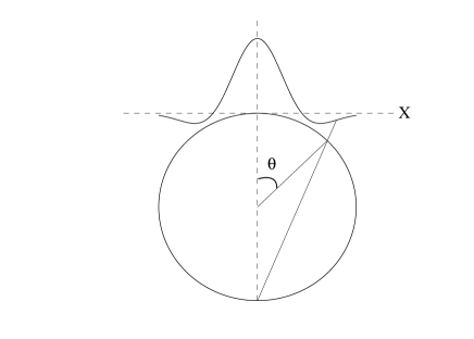
Figure 1: Stereographic projection to translate the properties of the Mexican Hat Wavelet from the plane to the sphere

Therefore, the isotropic wavelet $\Psi(x;R)$ transforms to

$$\Psi_{S}(\theta;R)\propto{(\cos\frac{\theta}{2})}^{-4}\Psi(x\equiv 2\tan\frac{\theta}{2};R).$$ (9)

It can be proven that the new wavelet on $S^{2}$ incorporates the basic properties, i. e. a) it is a compensated filter ($\int d\theta d\phi\sin\theta\Psi_{S}(\theta;R)=0$), b) translations are defined by translations along the sphere, i. e. rotations about the center of the sphere, c) the dilations are defined by the stereographic projection of dilations on the plane and d) for small angles one recovers the Euclidean limit.

a) Analysis

Let us consider a function on the sphere $f(\theta,\phi)$. The continuous wavelet transform with respect to $\Psi_{S}(\theta;R)$ is defined as the linear operation

$$\tilde{w}(\vec{x},R)=\int d\theta^{\prime}\,d\phi^{\prime}\sin\theta^{\prime}\,\tilde{f}(\vec{x}+\vec{\mu})\Psi_{S}(\theta^{\prime};R).\ \ \$$ (10)

$$\vec{x}\equiv 2\tan\frac{\theta}{2}(\cos\phi,\sin\phi),\ \ \ \vec{\mu}\equiv 2\tan\frac{\theta^{\prime}}{2}(\cos\phi^{\prime},\sin\phi^{\prime}),{}$$

$$\tilde{f}(\vec{x})\equiv f(\theta,\phi){},$$ (11)

$w(\theta,\phi;R)\equiv\tilde{w}(\vec{x},R)$ are the wavelet coefficients dependent on $3$ parameters.

b) Synthesis

A straightforward calculation based on the equation (5) leads, after stereographic projection, to the continuous reconstruction formula:

$$f(\theta,\phi)\equiv\tilde{f}(\vec{x})=\frac{1}{C_{\psi}}\int d\theta^{\prime}d\phi^{\prime}\sin\theta^{\prime}\frac{dR}{R^{3}}\tilde{w}(\vec{x}+\vec{\mu},R){}$$

$$\Psi_{S}(\theta^{\prime};R){}\ ,$$ (12)

where $\tilde{w}(\vec{x},R)\equiv w(\theta,\phi;R)$.

c) The MEXHAT wavelets

Figure 2: Mexican Hat Wavelet as deformed on the sphere (solid line) from the plane (dashed line). The scale of the wavelet is chosen to be $R=1$ rad.

A particular example is the MEXHAT wavelet defined by (see Figure 2)

$$\Psi(\theta;R)=\frac{1}{{(2\pi)}^{1/2}R\,N}{[1+{(\frac{y}{2})}^{2}]}^{2}[2-{(\frac{y}{R})}^{2}]e^{-{y}^{2}/2R^{2}},\ \ \$$ (13)

$$N(R)\equiv{(1+\frac{R^{2}}{2}+\frac{R^{4}}{4})}^{1/2},y\equiv 2\tan\frac{\theta}{2}.$$ (14)

We remark that the normalization constant has been chosen such that $\int d\theta d\phi\sin\theta\Psi^{2}(\theta;R)=1$. This is the wavelet we are going to use in this paper to analize non-Gaussianity associated to different models.

We comment that the stereographic projection of the MEXHAT wavelet has been recently used to analize maps of the cosmic microwave background radiation (CMB) (Cayón et al. 2001).

3 Spherical Haar Wavelets

SHW were introduced by Sweldens (1995) as a generalization of planar Haar wavelets to the pixelised sphere. They are orthogonal and adapted to a given pixelisation of the sky which must be hierarchical, contrary to the SMHW which are non-orthogonal and redundant. However they are not obtained from dilations and translations of a mother wavelet, contrary to planar Haar wavelets and SMHW. As for the planar Haar wavelets, they possess a good space-frequency localisation. However, their frequency localisation is not as good as that of the SMHW. Two applications of SHW to the analysis of CMB maps have already been performed. Tenorio et al. (1999) apply them to simulated CMB skies on the QuadCube pixelisation. They study the CMB spatial structure by defining a position-dependent measure of power. Also they show their efficiency in denoising and compressing CMB data. Barreiro et al. (2000) tested the Gaussianity of the COBE-DMR data on the HEALPix pixelisation. One of the advantages of HEALPix over QuadCube is that there is no need to correct for the pixel area.

Since detailed description of the SHW transform has already been given in the previous papers, we here describe the main features of the wavelet decomposition. The SHW decomposition is based on one scaling $\phi_{j,k}$ and three wavelet functions $\psi_{m,j,k}$ at each resolution level j and position on the grid k. For HEALPix the resolution is given in terms of the number of divisions in which each side of the basic 12 pixels is divided, $N_{side}=2^{j-1}$. Thus, for level $j$ the total number of pixels with area $\mu_{j}$ is given by $n_{j}=12\times 4^{j-1}$. Each pixel k at resolution j, $S_{j,k}$ is divided into four pixels $S_{j+1,k_{0}},...,S_{j+1,k_{3}}$ at resolution j+1. For computational reasons the maximum resolution we will consider in our simulations is $J=9$ which corresponds to $N_{side}=256$. The scaling and wavelet functions are simply given by

$$\phi_{j,k}(x)=\left\{\begin{array}[]{ll}1&ifx\in S_{j,k}\\ 0&otherwise\ ,\end{array}\right.$$ (15)

$$\psi_{1,j,k}=\frac{\phi_{j+1,k_{0}}+\phi_{j+1,k_{2}}-\phi_{j+1,k_{1}}-\phi_{j+1,k_{3}}}{4\mu_{j+1}}$$ (16)

$$\psi_{2,j,k}=\frac{\phi_{j+1,k_{0}}+\phi_{j+1,k_{1}}-\phi_{j+1,k_{2}}-\phi_{j+1,k_{3}}}{4\mu_{j+1}}$$ (17)

$$\psi_{3,j,k}=\frac{\phi_{j+1,k_{0}}+\phi_{j+1,k_{3}}-\phi_{j+1,k_{1}}-\phi_{j+1,k_{2}}}{4\mu_{j+1}}$$ (18)

where $k_{0},k_{1},k_{2},k_{3}$ are the four pixels at resolution level $j+1$ in which the pixel $k$ at level $j$ is divided. Please note that the three wavelet functions so defined differ from the ones used by Tenorio et al (1999) and Barreiro et al. (2000). We choose those expressions by similarity with the diagonal, vertical and horizontal details defined on the plane. The reconstruction of the temperature field is obtained by

$$\frac{\Delta T}{T}(x_{i})=\sum_{l=0}^{n_{j_{0}}-1}\lambda_{j_{0},l}\phi_{j_{0},j}(x_{i})+\sum_{m}\sum_{j=j_{0}}^{J-1}\sum_{l=0}^{n_{j}-1}\gamma_{m,j,l}$$

$$\psi_{m,j,l}(x_{i})\ ,$$ (19)

where $\lambda_{j_{0},k}$ and $\gamma_{m,j,k}$ are the approximation and detail coefficients respectively. The level index $j$ goes from the finest resolution $J$ to the coarsest one considered $j_{0}$.

Figure 3: Hierarchical structure of Wavelet coefficients for the Spherical Haar Wavelet.

The wavelet coefficients at level $j$ can be obtained from the four corresponding approximation coefficients at level $j+1$, $\lambda_{j+1,k_{i}}$ as follows (see figure 3.):

$$\lambda_{j,k}=\frac{1}{4}\sum_{i=0}^{3}\lambda_{j+1,k_{i}}$$ (20)

$$\gamma_{1,j,k}=\mu_{j+1}(\lambda_{j+1,k_{0}}+\lambda_{j+1,k_{2}}-\lambda_{j+1,k_{1}}-\lambda_{j+1,k_{3}})$$ (21)

$$\gamma_{2,j,k}=\mu_{j+1}(\lambda_{j+1,k_{0}}+\lambda_{j+1,k_{1}}-\lambda_{j+1,k_{2}}-\lambda_{j+1,k_{3}})$$ (22)

$$\gamma_{3,j,k}=\mu_{j+1}(\lambda_{j+1,k_{0}}+\lambda_{j+1,k_{3}}-\lambda_{j+1,k_{1}}-\lambda_{j+1,k_{2}})\ \ .$$ (23)

The generation of coefficients start with the original map, finest resolution $j=J$, for which the coefficients $\lambda_{J,k}$ are identified with the temperature fluctuation at pixel $k$.

Finally, from the definition of the SHW it is easily seen that this wavelet is not rotationally invariant, contrary to the SMHW.

4 Non-Gaussian simulations

There are many ways in which physically motivated non-Gaussian features can enter in the CMB temperature distribution. However, up to now there is no evidence of their existence, being all experimental data consistent with Gaussianity (Kogut et al. 1996, Barreiro et al. 2000, Aghanim et al. 2000, Cayón et al. 2001, Wu et al. 2001; see however Magueijo 2000 for a possible positive signal in the COBE-DMR data, although that detection has not been confirmed by any of the other analyses). If departures from Gaussianity of cosmological origin really exist they will more likely be small and all-sky, sensitive, arcminute resolution experiments will be needed for their detection.

Here the spherical wavelets will be tested against non-Gaussian simulations of artificially specified moments that will be assumed to be small. In this case a useful way to construct non-Gaussian distributions is by perturbing the Gaussian one through a sum of moments, the Edgeworth expansion. For simplicity we will consider the two lowest cumulants to characterise the deviations from normality: skewness and kurtosis. As discussed in the introduction alternative models to standard inflation, e.g. cosmic defects as a subdominant source of density perturbations or non-standard inflation, can produce significant levels of at least one of the two moments.

4.1 Edgeworth expansion

For small deviations from Gaussianity, there is a wide class of distributions that can be given in terms of a Gaussian distribution times an infinite sum of its cumulants. This is the well known Edgeworth expansion. The problem with this expansion is that setting all cumulants to zero except one does not guarantee the positive definiteness and normalization that a distribution has to satisfy. However, for small deviations from normality the resulting function is always positive at least up to many sigmas in the tail of the distribution and the normalization factor required for the function to become a well defined distribution is very small and does not appreciably disturb the non-zero moments (i.e. skewness or kurtosis) introduced in the first place.

The Edgeworth expansion can be obtained from the characteristic function $\phi(t)$ by considering the linear terms in the cumulants and performing the inverse Fourier transform to recover the density function $f(x)$:

$$f(x)=G(x)\bigl{\{}1+\sum_{n=3}^{\infty}\frac{k_{n}}{n!2^{n/2}}H_{n}\bigl{(}\frac{x}{\sqrt{2}}\bigr{)}+O(k_{n}k_{n^{\prime}})\bigr{\}}\ \ ,$$ (24)

where $H_{n}$ is the Hermite polynomial. Considering the perturbations corresponding to the skewness and kurtosis and keeping only the first terms in the corresponding Hermite polynomials, we have

$$f_{S}(x)=\frac{e^{-\frac{x^{2}}{2}}}{\sqrt{2\pi}}\Bigl{(}1+\frac{S}{6}\bigl{(}x(x^{2}-3)\bigr{)}\Bigr{)}\ ,$$ (25)

$$f_{K}(x)=\frac{e^{-\frac{x^{2}}{2}}}{\sqrt{2\pi}}\Bigl{(}1+\frac{K}{24}(x^{4}-6x^{2}+3)\Bigr{)}\ ,$$ (26)

where S, K denote skewness and kurtosis, respectively. We will use these equations to generate our artificially specified non-Gaussian distributions. Since the resulting distribution is not well defined even for the case of small skewness and kurtosis we set the function to zero when it becomes negative and we also normalize it appropriately. We remark that the zero cuts of the distribution, if present, appear far away in the tails of the distribution for the case of small values of skewness and kurtosis that we consider here. Also, as a consequence, the normalization value required is very close to 1. In this way we checked that the initial values of the skewness and kurtosis we start with in the Edgeworth expansion does not appreciably change after the necessary changes introduced to obtain a well defined probability density function (pdf).

In order to make the simulations resemble the CMB data observed by a given experiment we smooth them with a Gaussian filter. For practical reasons we use a FWHM of $33^{\prime}$ which may correspond to some of the channels in all-sky experiments like MAP and Planck (e.g. the $30$GHz channel of the Planck mission). We choose to work on the HEALPix pixelisation of the sphere with a resolution $N_{side}=256$. We use the HEALPix package to perform the analysis of our simulated CMB data. However, it is not adequate to use that package to convolve our unfiltered independent temperature data with the Gaussian $33^{\prime}$ FWHM beam in Fourier space, instead we perform the convolution in real space. After that, in order to make the simulations more realistic we normalize the CMB power spectrum $C_{l}$ of both Gaussian and non-Gaussian simulations to that of a CDM flat $\Lambda$-model using the HEALPix package. As a consequence of the beam convolution and the introduction of correlations in the temperature maps the original levels of skewness and kurtosis injected through the Edgeworth expansion are reduced (compare columns 1 and 2 in table 2). The performance of spherical wavelets will be tested with these simulations in section 5.

4.2 Distribution of spherical wavelet coefficients

Since wavelet coefficients represent linear transformations of the original data, in the case of a Gaussian distribution the wavelet coefficients remain Gaussian distributed. This a very nice property of wavelets and all we have to do to test Gaussianity in wavelet space is to look from deviations from normality.

However, for the case of the sphere any given pixelisation scheme will introduce biases. The specific bias introduced will depend on, for instance, whether the pixels are not of equal area or the distances between one pixel and its neighbours vary with the position on the sphere. This is in fact the situation for the two pixelisations already used to analyse all-sky CMB temperature fluctuations. For the COBE-DMR experiment the pixelisation used was the Quad-Cube and in this projection of the cube on the sphere equal-area pixels on the sides of the cube appear with different area when projected on the sphere. For present satellite experiments like MAP and Planck the HEALPix pixelisation is now widely used. While this pixelisation possesses very nice properties, such as equal area iso-latitude pixels, however the distances between one pixel and its neighbours vary with latitude. Pixels near the equator tend to be more uniformly distributed than those near the poles. As we will compute in next section, this property produces a bias in the kurtosis of the wavelet coefficients for the case of the SHW (see table 1, Gaussian case which corresponds to a null injected value for the kurtosis). For the Gaussian and non-Gaussian simulations which will be performed in next section we will compute the first cumulants of the coefficients of the two spherical wavelets considered in this paper for the HEALPix scheme. For the SHW the coefficients correspond to three different details: diagonal, vertical and horizontal. Since those details are directly obtained from linear operations of the four neighbour pixels (as we saw in the previous section) and pixels are not equally separated all over the sphere, correlations present in the temperature fluctuations make the wavelet coefficients to be biased. This bias produces a peaked distribution with respect to a Gaussian and therefore a positive kurtosis in the three details of the SHW coefficients even for temperature realizations derived from normal distributions (as can be seen from table 1, the mean value of the kurtosis for the finest resolution of the Gaussian model is displaced about $10\sigma$ from zero).

In the case of the SMHW we only have a type of coefficients for each scale. Since this is a continuous, rotationally invariant wavelet -and thus not adapted to the pixelisation- no bias is produced in this case.

Table 1: Mean and standard deviation, within parenthesis, for the different wavelet scales.

Injected

Wavelet

SMHW

SHW

Temperature

Scale

vert

diag

hori

SKEWNESS

0.00	1 pix	-1.0$\times 10^{-4}$(5.6$\times 10^{-3}$)	-1.3$\times 10^{-4}$(7.6$\times 10^{-3}$)	1.7$\times 10^{-4}$(5.5$\times 10^{-3}$)	-2.1$\times 10^{-4}$(7.3$\times 10^{-3}$)	-1.1$\times 10^{-3}$(2.3$\times 10^{-2}$)
	2 pix	-1.0$\times 10^{-4}$(6.3$\times 10^{-3}$)	-3.0$\times 10^{-4}$(1.1$\times 10^{-2}$)	7.3$\times 10^{-5}$(9.8$\times 10^{-3}$)	7.2$\times 10^{-5}$(1.1$\times 10^{-2}$)
0.00*	1 pix	-2.1$\times 10^{-5}$(3.4$\times 10^{-3}$)	2.1$\times 10^{-4}$(5.6$\times 10^{-3}$)	-3.1$\times 10^{-4}$(5.3$\times 10^{-3}$)	-1.0$\times 10^{-5}$(5.5$\times 10^{-3}$)	-4.8$\times 10^{-4}$(6.7$\times 10^{-3}$)
	2 pix	-1.7$\times 10^{-4}$(5.9$\times 10^{-3}$)	-7.8$\times 10^{-4}$(1.1$\times 10^{-2}$)	8.8$\times 10^{-4}$(1.1$\times 10^{-2}$)	1.1$\times 10^{-4}$(1.1$\times 10^{-2}$)
0.05	1 pix	1.3$\times 10^{-2}$(5.0$\times 10^{-3}$)	-2.7$\times 10^{-4}$(6.9$\times 10^{-3}$)	-1.7$\times 10^{-3}$(5.5$\times 10^{-3}$)	2.8$\times 10^{-4}$(7.2$\times 10^{-3}$)	9.0$\times 10^{-3}$(2.4$\times 10^{-2}$)
	2 pix	7.5$\times 10^{-3}$(6.1$\times 10^{-3}$)	-1.6$\times 10^{-3}$(1.1$\times 10^{-2}$)	-4.7$\times 10^{-4}$(9.3$\times 10^{-3}$)	2.0$\times 10^{-6}$(1.2$\times 10^{-2}$)
0.10	1 pix	2.7$\times 10^{-2}$(5.2$\times 10^{-3}$)	2.8$\times 10^{-4}$(7.1$\times 10^{-3}$)	-3.9$\times 10^{-3}$(5.6$\times 10^{-3}$)	6.0$\times 10^{-5}$(7.3$\times 10^{-3}$)	1.6$\times 10^{-2}$(2.3$\times 10^{-2}$)
	2 pix	1.5$\times 10^{-2}$(6.1$\times 10^{-3}$)	5.7$\times 10^{-4}$(1.1$\times 10^{-2}$)	-1.4$\times 10^{-3}$(9.6$\times 10^{-3}$)	-6.3$\times 10^{-4}$(1.1$\times 10^{-2}$)
0.30	1 pix	7.6$\times 10^{-2}$(5.4$\times 10^{-3}$)	2.6$\times 10^{-4}$(7.3$\times 10^{-3}$)	-1.0$\times 10^{-2}$(5.6$\times 10^{-3}$)	3.8$\times 10^{-4}$(7.7$\times 10^{-3}$)	4.6$\times 10^{-2}$(2.4$\times 10^{-2}$)
	2 pix	4.3$\times 10^{-2}$(6.0$\times 10^{-3}$)	6.7$\times 10^{-5}$(1.1$\times 10^{-2}$)	-3.3$\times 10^{-3}$(9.5$\times 10^{-3}$)	5.6$\times 10^{-4}$(1.1$\times 10^{-2}$)
0.30*	1 pix	9.5$\times 10^{-3}$(3.5$\times 10^{-3}$)	3.5$\times 10^{-5}$(5.4$\times 10^{-3}$)	-4.0$\times 10^{-4}$(5.7$\times 10^{-3}$)	-2.0$\times 10^{-4}$(5.8$\times 10^{-3}$)	1.1$\times 10^{-2}$(6.8$\times 10^{-3}$)
	2 pix	3.1$\times 10^{-2}$(6.2$\times 10^{-3}$)	2.4$\times 10^{-4}$(1.0$\times 10^{-2}$)	4.6$\times 10^{-6}$(1.1$\times 10^{-2}$)	9.9$\times 10^{-5}$(1.1$\times 10^{-2}$)
0.50	1 pix	1.2$\times 10^{-1}$(5.4$\times 10^{-3}$)	-5.6$\times 10^{-4}$(7.6$\times 10^{-3}$)	-1.6$\times 10^{-2}$(5.6$\times 10^{-3}$)	-6.4$\times 10^{-6}$(7.4$\times 10^{-3}$)	6.9$\times 10^{-2}$(2.4$\times 10^{-2}$)
	2 pix	6.6$\times 10^{-2}$(6.2$\times 10^{-3}$)	-5.9$\times 10^{-4}$(1.1$\times 10^{-2}$)	-5.4$\times 10^{-3}$(9.6$\times 10^{-3}$)	2.1$\times 10^{-5}$(1.1$\times 10^{-2}$)

KURTOSIS

0.00	1 pix	-3.6$\times 10^{-4}$(1.0$\times 10^{-2}$)	1.7$\times 10^{-1}$(2.0$\times 10^{-2}$)	1.8$\times 10^{-1}$(1.8$\times 10^{-2}$)	1.7$\times 10^{-1}$(1.9$\times 10^{-2}$)	-3.4$\times 10^{-3}$(2.6$\times 10^{-2}$)
	2 pix	-4.1$\times 10^{-4}$(1.2$\times 10^{-2}$)	1.0$\times 10^{-1}$(2.7$\times 10^{-2}$)	3.9$\times 10^{-2}$(2.5$\times 10^{-2}$)	1.0$\times 10^{-1}$(2.7$\times 10^{-2}$)
0.00*	1 pix	-8.7$\times 10^{-5}$(6.4$\times 10^{-3}$)	4.1$\times 10^{-3}$(1.6$\times 10^{-2}$)	-5.7$\times 10^{-5}$(1.1$\times 10^{-2}$)	4.4$\times 10^{-3}$(1.5$\times 10^{-2}$)	-1.1$\times 10^{-3}$(6.9$\times 10^{-3}$)
	2 pix	-9.7$\times 10^{-4}$(9.5$\times 10^{-3}$)	1.9$\times 10^{-2}$(2.3$\times 10^{-2}$)	1.9$\times 10^{-3}$(2.2$\times 10^{-2}$)	2.1$\times 10^{-2}$(2.3$\times 10^{-2}$)
0.10	1 pix	9.9$\times 10^{-3}$(1.0$\times 10^{-2}$)	1.7$\times 10^{-1}$(1.9$\times 10^{-2}$)	1.8$\times 10^{-1}$(1.8$\times 10^{-2}$)	1.7$\times 10^{-1}$(2.0$\times 10^{-2}$)	3.2$\times 10^{-3}$(2.6$\times 10^{-2}$)
	2 pix	3.9$\times 10^{-3}$(1.3$\times 10^{-2}$)	1.1$\times 10^{-1}$(2.7$\times 10^{-2}$)	4.1$\times 10^{-2}$(2.6$\times 10^{-2}$)	1.1$\times 10^{-1}$(2.8$\times 10^{-2}$)
0.30	1 pix	2.9$\times 10^{-2}$(1.0$\times 10^{-2}$)	1.8$\times 10^{-1}$(2.0$\times 10^{-2}$)	1.9$\times 10^{-1}$(1.8$\times 10^{-2}$)	1.8$\times 10^{-1}$(1.9$\times 10^{-2}$)	7.7$\times 10^{-3}$(2.7$\times 10^{-2}$)
	2 pix	1.2$\times 10^{-2}$(1.3$\times 10^{-2}$)	1.1$\times 10^{-1}$(2.7$\times 10^{-2}$)	4.8$\times 10^{-2}$(2.6$\times 10^{-2}$)	1.1$\times 10^{-1}$(2.8$\times 10^{-2}$)
0.40	1 pix	3.8$\times 10^{-2}$(1.1$\times 10^{-2}$)	1.9$\times 10^{-1}$(2.0$\times 10^{-2}$)	1.9$\times 10^{-1}$(1.8$\times 10^{-2}$)	1.9$\times 10^{-1}$(2.0$\times 10^{-2}$)	1.1$\times 10^{-2}$(2.7$\times 10^{-2}$)
	2 pix	1.7$\times 10^{-2}$(1.3$\times 10^{-2}$)	1.1$\times 10^{-1}$(2.8$\times 10^{-2}$)	5.3$\times 10^{-2}$(2.6$\times 10^{-2}$)	1.2$\times 10^{-1}$(2.8$\times 10^{-2}$)
0.50	1 pix	4.8$\times 10^{-2}$(1.1$\times 10^{-2}$)	1.9$\times 10^{-1}$(2.0$\times 10^{-2}$)	2.0$\times 10^{-1}$(1.8$\times 10^{-2}$)	1.9$\times 10^{-1}$(2.0$\times 10^{-2}$)	1.4$\times 10^{-2}$(2.6$\times 10^{-2}$)
	2 pix	2.1$\times 10^{-2}$(1.3$\times 10^{-2}$)	1.2$\times 10^{-1}$(2.8$\times 10^{-2}$)	5.3$\times 10^{-2}$(2.5$\times 10^{-2}$)	1.2$\times 10^{-1}$(2.8$\times 10^{-2}$)
0.50*	1 pix	2.8$\times 10^{-3}$(6.2$\times 10^{-3}$)	1.6$\times 10^{-3}$(1.1$\times 10^{-2}$)	-5.7$\times 10^{-4}$(1.2$\times 10^{-2}$)	-8.1$\times 10^{-4}$(1.1$\times 10^{-2}$)	2.3$\times 10^{-3}$(7.2$\times 10^{-3}$)
	2 pix	1.2$\times 10^{-2}$(9.1$\times 10^{-3}$)	2.3$\times 10^{-2}$(2.2$\times 10^{-2}$)	1.4$\times 10^{-3}$(2.2$\times 10^{-2}$)	2.3$\times 10^{-2}$(2.4$\times 10^{-2}$)

∗These models include the addition of noise to the maps with S/N = 1.

5 Discriminating power

The discriminating power of the spherical wavelets will be tested using Gaussian and non-Gaussian simulations with different amounts of either skewness or kurtosis introduced using the Edgeworth expansion, and normalized to a power spectrum $C_{l}$ consistent with observations (as discussed above). Since the skewness and kurtosis are introduced at the highest resolution through the Edgeworth expansion (as described above), we expect to detect them with the skewness and kurtosis of the spherical wavelet coefficients also at the highest resolutions. Thus we will consider for the analysis the first five resolution scales starting from the finest one. The scales go as powers of 2 for the SHW and for comparison we choose the same values for the SMHW parameter $R$: 1, 2, 4, 8 and 16 pixels. We can relate the scales of the two wavelets by looking to the scaling functions. The relation between the side, $s$, of the step function (scaling function for the Haar wavelet) and the dispersion $R$ of the Gaussian is: $s=\sqrt{2\pi}R$. Then, for the finest scale $s=2$ pixels, which corresponds to an $R\approx 0.8$ pixels which is approximately 1 pixel.

Results obtained in Fourier space are equivalent to those obtained in real space if the functions considered are bandwidth limited (with the bandwidth included in the one covered by the pixelisation). We have checked this for the finest resolution of the SMHW. The average difference between the SMHW coefficients computed by direct convolution in real space and going to Fourier space is $<1\%$.

Given the 5 values of skewness or kurtosis corresponding to the 5 resolution scales for the SMHW and the 15 values for the SHW (5 scales for each of the 3 details), we would like to construct a test statistic which, combining all this information, can best distinguish between the two hypotheses: a) $H_{0}$: the data are drawn from a Gaussian model, b) $H_{1}$: the data are drawn from a non-Gaussian model with either skewness or kurtosis. The best test statistic in the sense of maximum power for a given significance level is given by the likelihood ratio:

$$t(\vec{x})=\frac{f(\vec{x}|H_{0})}{f(\vec{x}|H_{1})}$$ (27)

where $f(\vec{x}|H_{0})$ and $f(\vec{x}|H_{1})$ are the pdf of the data given hypotheses $H_{0}$ and $H_{1}$, respectively. Since we do not know those multivariate pdf s and would be tremendously costly in cpu time to determine them by Monte Carlo simulations, we use as test statistic the simpler Fisher linear discriminant function (Fisher 1936; see also Cowan 1998). This discriminant has been recently used by Barreiro and Hobson (2001) to study the discriminanting power of planar wavelets to detect non-Gaussianity in the CMB in small patches of the sky. The Fisher discriminant is a linear function of the data that maximizes the distance between the two pdf’s, $g(t|H_{0})$ and $g(t|H_{1})$, such a distance defined as the ratio $(\tau_{0}-\tau_{1})^{2}/(\Sigma_{0}^{2}+\Sigma_{1}^{2})$. $\tau_{k}$ and $\Sigma_{k}^{2}$, $k=0,1$, are the mean and the variance of $g(t|H_{k})$, respectively. The Fisher discriminant is given by:

$$t(\vec{x})=(\vec{\mu}_{0}-\vec{\mu}_{1})^{T}W^{-1}\vec{x}$$ (28)

with $W=V_{0}+V_{1}$ and $V_{k}$ the covariance matrix and $\vec{\mu}_{k}$ the mean values of $f(\vec{x}|H_{k})$. In the particular case that $f(\vec{x}|H_{0})$ and $f(\vec{x}|H_{1})$ are both multidimensional Gaussians with the same covariance matrix, the Fisher discriminant is equivalent to the likelihood ratio.

The mean values and covariance matrices of the skewness and kurtosis at each resolution level for the Gaussian and non-Gaussian models are obtained from a large number of simulations. In the next section we use those simulations to compare the power of the test $p\equiv 1-\beta$ to discriminate against the alternative hypothesis $H_{1}$ at a given significance level $\alpha$ for the two spherical wavelets. $\alpha$ and $\beta$ account for the probability of rejecting the null hypothesis $H_{0}$ when it is actually true (error of the first kind) and the probability of accepting $H_{0}$ when the true hypothesis is $H_{1}$ and not $H_{0}$ (error of the second kind), respectively. The decision to accept or reject $H_{0}$ is done by defining a critical region for the statistic $t$; if the value of $t$ is greater than a cut value $t_{cut}$ the hypothesis $H_{0}$ is rejected. Thus, $\alpha$ and $\beta$ are given by:

$$\alpha=\int_{t_{cut}}^{\infty}dtg(t|H_{0})\ ,$$ (29)

$$\beta=\int_{-\infty}^{t_{cut}}dtg(t|H_{1})\ .$$ (30)

This kind of analysis is very much along the lines of the one performed by Barreiro and Hobson (2001) for planar wavelets. From now on a value for the sensitivity of $\alpha=1\%$ will be adopted.

6 Results

Table 2: Power of the Fisher discriminant at 1% significance level

	Injected	True1	SMHW	SHW	Temperature
		$\times 10^{-2}$	P(%)	P(%)	P(%)
	0.05	0.9(2.4)	66.8	1.51	2.51
	0.10	1.6(2.3)	100	7.09	4.67
SKEWNESS	0.30	4.6(2.4)	100	36.12	36.85
	0.302	1.1(0.7)	99.6	1.80	2.83
	0.50	6.9(2.4)	100	78.46	73.6
	0.10	0.3(2.6)	15.35	3.00	1.42
	0.30	0.8(2.7)	86.89	9.00	3.40
KURTOSIS	0.40	1.1(2.7)	98.10	16.11	4.90
	0.50	1.4(2.6)	99.90	28.43	3.50
	0.502	0.2(0.7)	20.84	1.00	0.32

• True refers to the mean value obtained in the analysed maps. The standard deviation is given within parenthesis.

• These models include the addition of noise to the maps with S/N = 1.

For both, Gaussian and not Gaussian models, we perform a $1000$ simulations. As commented above, to make the simulations more realistic each simulation is convolved with a Gaussian filter of $33^{\prime}$. In addition, its power spectrum $C_{l}$ is normalized to that of a CDM flat $\Lambda$-model using the HEALPix package. For each of the simulations the wavelet coefficients for both the SMHW and the SHW are computed. The SMHW coefficients are computed by convolving the CMB map with the SMHW given in eq. (13). We again use the HEALPix package to perform such convolution in Fourier space, having previously calculated the Legendre coefficients of the SMHW at the specified resolution. The SHW detail coefficients are computed by performing the linear combinations of 4 pixels as described in section 3. Computation time of wavelet coefficients using HEALPix scale as $N^{3}_{N_{side}}$ and $N^{2}_{N_{side}}$ for SMHW and SHW respectively.

Figure 4: Comparison of Mexican Hat wavelet (black circle) and the Haar Wavelet details: Vertical (diamond), Diagonal (triangle) and Horizontal (square); for Kurtosis (left) and Skewness (right) values of 0.1, 0.3 and 0.5 (from top to bottom). Each point represents the number of sigmas deviated from the Gaussian model. Also plotted is the stripe for the non-Gaussianity determined from the temperature map (in this case only the pixel scale is meaninful, the stripe is drawn only for illustrative purposes).

In figure 4 we show the mean values and dispersion of the skewness and kurtosis of the Gaussian and non-Gaussian models for the temperature map, and for the first $5$ resolution levels of the SHW diagonal, vertical and horizontal coefficients and SMHW coefficients. As expected the differences are best seen in the finer resolutions. It is clear from figure 4 that the differences in the skewness for the two models are more remarkable for the SMHW than for the SHW and the temperature map. This is also the case for the kurtosis. As we pointed out in section 4.2, there is a strong bias in the kurtosis of the three details of the SHW coefficients due to the slight non-uniform distribution of pixels on the sphere in the HEALPix pixelisation. This kind of bias is expected for any pixelisation of the sphere due to the impossibility of having a uniform pixelisation. The specific bias introduced will depend on the pixelisation scheme used. On the contrary, no bias is present for the SMHW coefficients due to its continuous nature.

Figure 5: Fisher Discriminant for Skewness from Spherical Haar Wavelet (left) and Spherical Mexican Hat Wavelet (right). From top to bottom, the values of skewness in the original maps are 0.1, 0.3 and 0.5. The solid line is the Gaussian model, while the dashed one represents the non-Gaussian case.

Figure 6: Fisher Discriminant for Kurtosis from Spherical Haar Wavelet (left) and Spherical Mexican Hat Wavelet (right). From top to bottom, the values of kurtosis in the original maps are 0.1, 0.3 and 0.5. The solid line is the Gaussian model, while the dashed one represents the non-Gaussian case. Please note the bias in the distribution of the SHW kurtosis as discussed in the text.

The Fisher discriminant $t$ can still be applied to distinguish between the two models even in the presence of that bias in the kurtosis. As seen in the previous section, what enters in the linear coefficients to compute the statistic $t$ is the difference between the means from the two models, cancelling out the bias term. In figures 5,6 we show the pdf s of the statistic $t$ for three values of the skewness and kurtosis of the non-Gaussian models. It is clear that for both non-Gaussian models, with either positive skewness or kurtosis, the SMHW is able to distinguish between the Gaussian and non-Gaussian models much better than the SHW.

In table 2 the power $p$ of the Fisher discriminant constructed from the skewness or kurtosis of the SMHW, SHW and temperature is given for several values of the cumulants. For the case of the temperature of the map the statistic is given directly by its cumulants. Again, the performance of the SMHW is superior to the SHW and the temperature in all cases.

Figure 7: Top graphics: Comparison of Mexican Hat wavelet (black circle) and the Haar Wavelet details: vertical (diamond), diagonal (triangle) and horizontal (square); for skewness 0.3 (right) and kurtosis 0.5 (left) with added noise. Each point represents the number of sigmas deviated from the Gaussian model with noise. Also plotted is the stripe for the non-Gaussianity determined from the temperature map (in this case only the pixel scale is meaninful, the stripe is drawn only for illustrative purposes). Bottom graphics: Fisher discriminant for skewness (right) and kurtosis (left) from Spherical Haar and Mexican Hat Wavelets

Since the SHW is affected by the non-uniform pixelisation of the sphere, one might wonder if its failure to detect non-Gaussianity is a feature of the Haar wavelet in general or a consequence of the pixel dependent scale mixing. In order to answer this question we have made the same comparison between Gaussian and non-Gaussian models, one with skewness 0.3 and the other with kurtosis 0.3, but now on the plane. (We have considered simulated $12^{\odot}.8\times 12^{\odot}.8$ maps with $1^{\prime}.5$ pixels and a beam of $5^{\prime}$ FWHM. The steps of the simulation and analysis are the same as for the sphere). The result is very similar to the one found on the sphere. Therefore, the failure of the Haar wavelet to detect non-Gaussianity is an intrinsic caracteristic of this wavelet and not a consequence of the pixel dependent scale mixing due to its implementation on the sphere. (Notice, however, that its performance can be similar to other planar wavelets for some specific features more adapted to its shape, e.g. cosmic strings, see Barreiro and Hobson 2001). The pixel dependent scale mixing basically induces a bias which has been taken into account in the analysis.

In order to know the effect of instrumental noise (white) on the discriminating power of the spherical wavelets we have also added noise to the temperature maps with an amplitude equals to the signal, $S/N=1$. In this case 500 simulations were generated. As shown in figure 7, the first resolution scale is the most affected and now the second scale is the most relevant for discrimination between models. In this figure it is also plotted the new pdf’s for the Fisher discriminant for $30\%$ injected skewness and $50\%$ injected kurtosis. The noise effect is shown in the narrowing of the separation between distributions as compared to the no-noise case. We see that the SMHW is still able to discriminate with a high power for the skewness model with a skewness value in the analysed map of $1.1\%$. For the kurtosis model, the addition of noise with the same amplitude than the signal reduces the level of kurtosis in the analysed map from $1.4\%$ to $0.2\%$, a level too low to be detectable.

Finally, even if future experiments like MAP and Planck observe the full sky probably only the fraction outside the Galactic plane will be used to test non-Gaussianity. This problem has already been considered in previous papers analysing the Gaussianity of the COBE-DMR data with the SHW and the SMHW (Barreiro et al. 2000, Cayón et al. 2001). As can be seen from those papers the impact on the two methods is similar (in both cases one looses all the coefficients computed from pixels intersecting the cut). In any case, for future missions like MAP or Planck, the Galactic cut should be much smaller than for COBE because of the much better resolution and the much larger frecuency information, implying a smaller impact on the analysis.

7 Conclusions

We have compared the performance of the two spherical wavelet families already used to test the Gaussianity of the COBE-DMR CMB data: Mexican Hat (Cayón et al. 2001) and Haar (Barreiro et al. 2000). As testbed we use non-Gaussian simulations of all-sky arcminute resolution CMB maps, with a power spectrum $C_{l}$ consistent with observations and artificially specified amounts of skewness or kurtosis. Most, if not all, physically motivated non-Gaussian primordial models of structure formation proposed in the literature show some amounts of either of these two moments in the CMB maps. These simulated sky maps are pixelised using the widely used HEALPix package. As commented in section 4.2 any pixelisation scheme of the sphere will introduce a bias because of the impossibility of a uniform pixelisation. In particular, for the HEALPix scheme this bias shows up as a positive kurtosis in the Spherical Haar Wavelets (SHW) coefficients even for temperature realizations derived from normal distributions. The bias represents a $\approx 10\sigma$ effect for the finest resolution, as can be seen from the first row of the kurtosis in table 1. On the contrary no bias is present in the case of the Spherical Mexican Hat Wavelet (SMHW) due to its continues nature, i.e. not adapted to the pixelisation scheme.

The main conclusion of this paper is that the SMHW bases are much more efficient to discriminate between Gaussian and non-Gaussian models with either skewness or kurtosis present in the CMB maps than the Spherical Haar Wavelet (SHW) ones. More specifically, the SMHW is able to discriminate a $1.6\%$ skewness with a power of $100\%$ at the $1\%$ significance level whereas the SHW can weakly discriminate a $6.9\%$ skewness with a power of only $78\%$ at the same significance. In the case of kurtosis, the SMHW detects a $1.4\%$ level with a power of $99.9\%$ whereas for the SHW the power is only $28\%$, at the same $1\%$ significance level. The failure of the Haar wavelet to detect non-Gaussianity is not a consequence of the pixel dependent scale mixing due to its implementation on the sphere but an intrinsic property of this wavelet (as has been demonstrated by performing a similar analysis on the plane). If we were to use the temperature map instead of the wavelet coefficients, the power would be always smaller than for the wavelets (only comparable to the SHW in the case of skewness). An interesting property of the SMHW is that an injected skewness/kurtosis in the temperature maps produces an amplified skewness/kurtosis in the SMHW coefficients and a negligible kurtosis/skewness. On the contrary the SHW is not able to amplify any injected skewness/kurtosis with neither skewness nor kurtosis of its coefficients.

Finally, we have also tested the performance of the spherical wavelets in the more realistic case in which instrumental noise (white) is present in the maps. In this case the highest resolution scale is the most affected, being the best scale for discrimination the second one. For a signal to noise ratio $S/N=1$, and combining all the information from all the scales with the Fisher discriminant, the SMHW is still able to discriminate with a high power levels of skewness and kurtosis above $1\%$.

References

- [1] Aghanim, N., Forni, O. & Bouchet, F.R. 2000, astro-ph/0009463
- [2] Antoine, J.-P. & Vandergheynst, P., 1998, J. Math. Phys., 39, 3987
- [3] Barreiro, R.B. & Hobson, M.P. 2001, MNRAS, 327, 813 (astro-ph/0104300)
- [4] Barreiro, R.B., Martínez-González, E. & Sanz, J.L. 2001, MNRAS, 322, 411
- [5] Barreiro, R.B., Hobson, M.P., Lasenby, A.N, Banday, A.J., Górski, K.M. & Hinshaw, G. 2000, MNRAS, 318, 475
- [6] Bromley, B.C., Tegmark, M. 1999, ApJ, 524, L79
- [7] Cayón, L., Sanz, J. L., Barreiro, R. B., Vielva, P., Toffolatti, L., Silk, J., Diego, J. M. & Argueso, F., 2000, MNRAS, 315, 757
- [8] Cayón, L., Sanz, J.L., Martínez-González, E., Banday, A.J., Argeso, F., Gallegos, J.E., Gorski, K.M. & Hinshaw, G. 2001, MNRAS, 2001, 326, 1243.
- [9] Contaldi, C.R., Ferreira, P.G., Magueijo, J., Górski, K.M. 2000, ApJ, 534, 25
- [10] Coulson, D., Ferreira, P., Graham, P., Turok, N. 1994, Nature, 368, 27
- [11] Cowan, G., 1998, “Statistical Data Analysis”, Oxford University Press, Oxford
- [12] Diego, J.M., Martínez-González, E., Sanz, J.L., Mollerach, S. & Martínez, V.J. 1999, MNRAS, 306, 427
- [13] Ferreira, P.J., Magueijo, J. & Górski, K. 1998, ApJ, 503, L1
- [14] Fisher R.A., 1936, Ann. Eugen., 7, 179; reprinted in “Contributions to Mathematical Statistics”, 1950, Jonh Wiley, New York
- [15] Górski, K.M., Hivon, E. & Wandelt, B.D. (astro-ph/9812350) 1999, Proceedings of the MPA/ESO Conference on Evolution of Large-Scale Structure: from Recombination to Garching, 2-7 August 1998; eds. A.J. Banday, R.K. Sheth and L. Da Costa, PrintPartners IPSKAMP NL (1999)
- [16] Heavens, A.F., Gupta, S. 2001, MNRAS, 324, 960
- [17] Hobson, M.P., Jones, A.W. & Lasenby, A.N. 1999, MNRAS, 309, 125
- [18] Kaiser, N., Stebbins, A. 1984, Nature, 310, 391
- [19]
- [20] Komatsu, E. & Spergel, D.N. 2001, PRD, 63, 63002
- [21] Linde, A. & Mukhanov, V. 1997, PRD, 56, 535
- [22] Magueijo, J. 2000, ApJ, 528, L57
- [23] Marr, D. & Hildreth, E.C. 1980, Proc. Roy. Soc. London, Ser. B, No. 207, 187.
- [24] Mollerach, S., Martínez, V.J., Diego, J.M., Martínez-González, E., Sanz, J.L. & Paredes, S. 1999, ApJ, 525, 17
- [25] Mukherjee, P., Hobson, M.P. & Lasenby, A.N. 2000, MNRAS, 318, 1157
- [26] Naselsky, P.D., Novikov, D.I. 1998, ApJ, 507, 31
- [27] Netterfield, C.B. et al. 2001, astro-ph/0104460
- [28] Pando, J. Valls-Gabaud, D., Fang, L.Z. 1998, Phys.Rev.Lett., 81, 4568
- [29] Pryke, C. et al. 2001, astro-ph/0104490
- [30] Rocha, G. et al. 2000, astro-ph/0008070
- [31] Schmalzing, J. & Górski, K.M. 1998, MNRAS, 297, 355
- [32] Stompor, R. et al. 2001, astro-ph/0105062
- [33] Sweldens, W., 1996, Applied Comput. Harm. Anal., 3, 1186
- [34] Tenorio, L., Jaffe, A.H., Hanany, S. & Lineweaver, C.H. 1999, MNRAS, 310, 823
- [35] Turok, N, Spergel, D. 1990, PRL, 64, 2736
- [36] Verde, L., Wang, L., Heavens, A.F. & Kamionkowski, M. 2000, MNRAS, 313, 141
- [37] Vielva, P., Martínez-González, E., Cayón, L., Diego, J.M., Sanz, J.L., Toffolatti, L. 2001, MNRAS, 326, 181
- [38] Wu, J.H.P. et al. 2001, astro-ph/0104248