An Hi survey of the Centaurus and Sculptor Groups

We present results of two 21-cm H i surveys performed with the Australia Telescope Compact Array in the nearby Centaurus A and Sculptor galaxy groups. These surveys are sensitive to compact H i clouds and galaxies with H i masses as low as $\sim 3\times 10^{6}\ M_{\odot}$, and are therefore among the most sensitive extragalactic H i surveys to date. The surveys consist of sparsely spaced pointings that sample approximately 2% of the groups’ area on the sky. We detected previously known group members, but we found no new H i clouds or galaxies down to the sensitivity limit of the surveys. If the HI mass function had a faint end slope of $\alpha=1.5$ below $M_{HI}=10^{7.5}\ M_{\odot}$ in these groups, we would have expected $\sim 3$ new objects. Cold dark matter theories of galaxy formation predict the existence of a large number low mass DM sub-halos that might appear as tiny satellites in galaxy groups. Our results support and extend similar conclusions derived from previous H i surveys that a H i rich population of these satellites does not exist.

1 Introduction

The Cold Dark Matter (CDM) theory is currently widely accepted as the most successful theory for the formation of structure in the universe. It has, however, become clear of late that two important results that follow naturally from the CDM theory, are difficult to reconcile with observational data: 1) The central parts of galaxy halos should have high densities with cuspy distributions (e.g. Navarro, Frenk & White 1996, 1997; Moore et al. 1999a) and, 2) high mass galaxies should be surrounded by large numbers of compact, low-mass satellites (e.g. Moore et al. 1999b; Klypin et al. 1999).

With regard to the first problem, recent high-resolution rotation curves of a large sample of Low Surface Brightness (LSB) and dwarf galaxy rotation curves show that their dark matter distributions are best characterized by a central constant density core with a typical size of a few kpc (de Blok et al. 2001b). This is in sharp contrast with the CDM result which predicts that the central parts of galaxies are characterized by a central cusp with a density that increases sharply towards the center.

Another problem is that the number of low-mass satellites actually observed is much lower than predicted. For example, in the Local Group only $\sim 36$ dwarf galaxies are known, while CDM predicts several hundreds of these low-mass galaxies (e.g. Moore et al. 1999b; Klypin et al. 1999).

If the gas densities at the centers of these objects are high enough to prevent ionization by the metagalactic uv-background of a significant fraction of the innate hydrogen gas, they should be detectable at the present epoch in sensitive 21-cm H i emission line surveys.

This led to the hypothesis that the observed (compact) high velocity clouds (HVCs) are actually extra-galactic and candidates for the missing low mass halos (Blitz et al. 1999; Braun & Burton 1999). Typical median properties of the locally observed compact HVCs population as derived from the HIPASS data (Putman et al. 2002) are a size of $\sim 0.2$ degrees, a peak column density of $1.4\times 10^{19}$ cm^-2, a velocity width of 35 km s^-1 and a total flux density of 19.9 Jy km s^-1. If compact HVCs are truly extra-galactic then this implies a median H i mass of $M_{HI}=2.3\times 10^{6}\ M_{\odot}$ for a distance of $700$ kpc, or $M_{HI}=7.5\times 10^{5}\ M_{\odot}$ for a distance of 400 kpc. These H i clouds should also be present in other galaxy groups and, as the parameters above show, detectable. There has recently been a large effort to find them in existing and new H i surveys (Zwaan & Briggs 2000; Dahlem et al. 2001; Zwaan 2001; Verheijen et al. 2000). Groups are presently the only environments where it is feasible to search for these clouds as the overdensity of the groups increases the number of possible detections. Since in numerical simulations of hierarchical structure formation the number of low mass halos is scale-invariant, the same ratio of low mass halos to normal size galaxies is expected in groups and in the field. The surveys showed that HVC-like objects are not distributed throughout groups and galaxy halos on scales of $\sim 1$ Mpc (but see Braun & Burton 2001). The HVCs must therefore be much closer to our Milky Way Galaxy than Blitz et al. (1999) originally proposed and they are therefore insignificant contributors to the baryon and total mass content of groups and galaxies.

There is, however, still a region of parameter space that has not been surveyed extensively. H i surveys to date have been less suited to constrain the population of compact, high column density, low H i mass clouds and galaxies. If such a population were to exist, it could contain a substantial fraction of $\Omega_{\rm gas}(z=0)$ locked up in such low H i masses which would not have been detected in recent H i surveys (Rosenberg & Schneider 2000; Zwaan et al. 1997; Kilborn et al. 2000).

In this paper we present results of two surveys designed to probe the regime of compact, low H i mass objects. These surveys, conducted with the Australia Telescope Compact Array (ATCA), have the lowest H i mass sensitivity to date with high spatial and velocity resolution. Section 2 discussed the targets of our surveys; section 3 addresses the observations. In section 4 we discuss the results, and section 5 describes the implications for the space density of low-mass galaxies.

2 Targets

At 3.5 Mpc distance from the Milky Way, the Cen A group is one of the nearest gas-rich groups known. It is well-defined both in projection on the sky and in velocity (Côté et al. 1997). It contains a large variety of galaxies, including the well-known radio galaxy Cen A (NGC 5128). The largest members are generally early-type galaxies. A large number of dwarf galaxies is however known (Côté et al. 1997; Côté, Carignan, & Freeman 2000; Banks et al. 1999), making this group ideal for this kind of survey, due to its small distance as well as large over density.

The Sculptor group has different properties. It is dominated by a small number of gas-rich late-type spiral galaxies (e.g. Jerjen et al. 1998; Côté, Carignan, & Freeman 2000). Sculptor is thought to be an elongated collection of galaxies seen pole-on (Jerjen et al. 1998) and linked with the Local Group. Following Côté et al. (1997) we adopt a distance of 2.5 Mpc. A previous H i survey of the Scl group (Haynes & Roberts 1979) detected many H i clouds, but these are not associated with the group. Rather they belong to the Magellanic Stream and the Milky Way.

Côté et al. (1997) derive from their extended Cen A and Scl dwarf samples velocity dispersions of 150 and 202 $\rm km\,s^{-1}$ respectively. The equivalent crossing times are $4.5\times 10^{9}$ and $3.2\times 10^{9}$ years. This is in both cases a significant fraction of the Hubble time, showing that both groups are dynamically unevolved, loose structures.

3 Observations

We have observed regions in both the nearby Centaurus A group and the Sculptor group in H i with the ATCA. As we have used different observing strategies for each group we discuss them separately.

3.1 Centaurus

We observed part of the Cen A group at 21-cm using a grid of 36 pointings with the Australia Telescope Compact Array in the 750-D configuration. Figure 1 overlays the pointing centers on the distribution of member galaxies (Côté et al. 1997) on the sky. The grid includes M83, and several known dwarf galaxies, and a large underdensity located behind M83. We thus sample a variety of densities. Table 1 lists the coordinates of the pointing centres for all pointings. Pointings in the grid were spread 1 degree apart.

The grid was observed over 9 runs of 12 hours each (3-4 and 12-18 July 1999). In each 12 hour session one block of 4 pointing was observed by cycling over the 4 pointings in mosaicing mode (90 seconds per pointing per cycle). We used a bandwidth of 8 MHz divided into 1024 channels. The velocity range was 0 - 1700 km s^-1 giving a good coverage of the velocity spread of the galaxies in the group.

For each pointing a data cube was created measuring $256\times 256\times 785$ pixels and a pixel size of $16^{\prime\prime}\times 16^{\prime\prime}\times 2$ km s^-1, thus encompassing two primary beam FWHM per pointing. The average noise for all cubes was 10.3 mJy per channel (without Hanning smoothing; no primary beam correction was applied). Table 1 also lists the average noise for each cube separately. The minimum detectable H i mass per 2 km/s channel in a 3 hour integration is thus $\sim 3\times 10^{5}M_{\odot}$ ($5\sigma$) at the pointing center. For a velocity width of 20 km s^-1, the minimum detected H i mass would be $\sim 3\times 10^{6}$ $M_{\odot}$, assuming optimal velocity smoothing. The synthesized beam was $65^{\prime\prime}\times 48^{\prime\prime}$, corresponding to $\sim 1$ kpc at the distance of Cen A. The column density sensitivity ($5\sigma$) for each 2 $\rm km\,s^{-1}$ channel is $4\times 10^{19}$ cm^-2 or $8\times 10^{19}$ after smoothing to 10 $\rm km\,s^{-1}$.

As the grid points are spread 1 degree apart, and the primary beam FWHM of the Compact Array measures 35^′ at 21-cm, this grid will not give uniform sensitivity coverage, but that is specifically not the intention of this part of the experiment. For any (moderately) steep Hi Mass Function (HiMF) the number of low mass galaxies in a unit volume will be larger than the number of high mass galaxies. A larger volume thus needs to be probed in order to get good statistics on the high mass galaxies. However, high mass galaxies in general have larger fluxes and can be found out to a larger distance from the center of the primary beam than low-mass, low flux galaxies. By spreading out the grid points we are therefore able to probe the dwarfs in the central parts of the primary beam, while the outer parts of the primary beam will give us enough volume coverage to pick up sufficient high mass galaxies. This survey probes approximately 4% of the group volume at $M_{\rm HI}=10^{6}M_{\odot}$ and about 12% at $10^{7}M_{\odot}$ (since this mass can be detected at larger distances from the center of the primary beam). These numbers are based on a group radius of 0.64 Mpc (van den Bergh 2000)

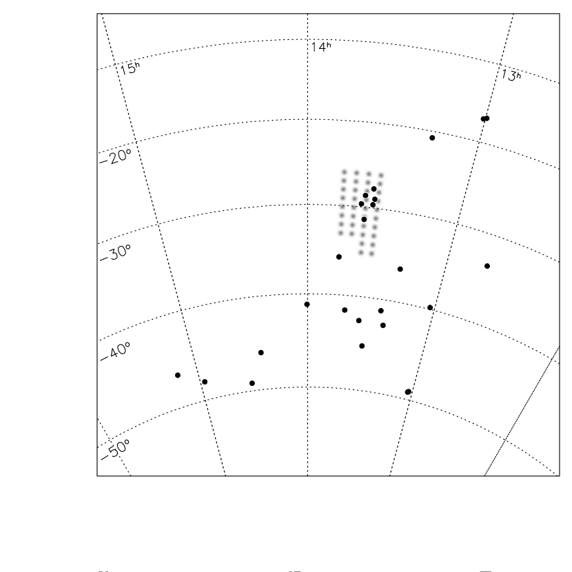
Figure 1: The observed grid on the sky of the Cen survey. Observed pointings are indicated by grey circles. Known galaxies from the catalog by Côté et al (1997) are indicated by black points.

This mode of observing probes a different area of parameter space than blind extragalactic H i surveys such as AHISS (Zwaan et al. 1997), HIPASS (Barnes et al. 2001) or ADBS (Rosenberg & Schneider 2000). These surveys are conducted with considerably coarser spatial and velocity resolution (for HIPASS $15^{\prime}$ and $13.2$ km s^-1 respectively), but with a large area coverage. They are excellent at picking up extended low surface brightness emission, e.g. local HVCs, but their coarse resolutions are insufficient to resolve e.g. small H i clouds in the close vicinity of other galaxies (Barnes & de Blok 2001). Their relatively coarse velocity resolutions furthermore make it difficult to distinguish narrow-velocity width (and presumably low-mass) galaxies from noise or interference spikes without further follow-up observations. Our current survey has much higher spatial and velocity resolution, but covers a smaller area. It does however enable us to look 10 times lower down the slope of the HiMF. A survey such as the current one is better suited to pick up compact and narrow-line width objects and is therefore complementary to the low resolution blind H i surveys.

3.2 Sculptor

Our original intention for the Scl survey was to image a large area with uniform sensitivity, with a fully sampled grid of pointings, as opposed to the Cen survey where the pointing were all independent. The motivation for this was to search in the volume between Sculptor and the Local Group. The Scl survey was done in the same observing session as the Cen survey, at those times when Cen was below the horizon.

We chose an area centered on $0^{h}30^{m},-30^{\circ}00^{\prime}$ which we observed using a hexagonal grid with a 19.6^′ distance between the pointings. In each 12h session, we observed 4 pointings, cycling over them every 15 min. We used a 4 MHz bandwidth, centered on a velocity of 500 km s^-1. Unfortunately, as the Scl survey happened in unallocated time, we were limited by telescope overrides and maintenance. This meant that we could observe only 22 pointings in a rather narrow strip and the area with uniform noise in the final mosaic thus proved to be rather small. In addition, some instrumental problems resulted in some pointings having a higher noise level. In the end we decided that the only way to get reliable statistics was to treat all pointings as independent pointings and proceed in the same manner as with the Cen survey. Table 1 lists the coordinates of the 22 pointings that we observed. Fig. 2 shows their lay-out on the sky. Also shown are the positions of the Sculptor group members (Jerjen et al. 2000)

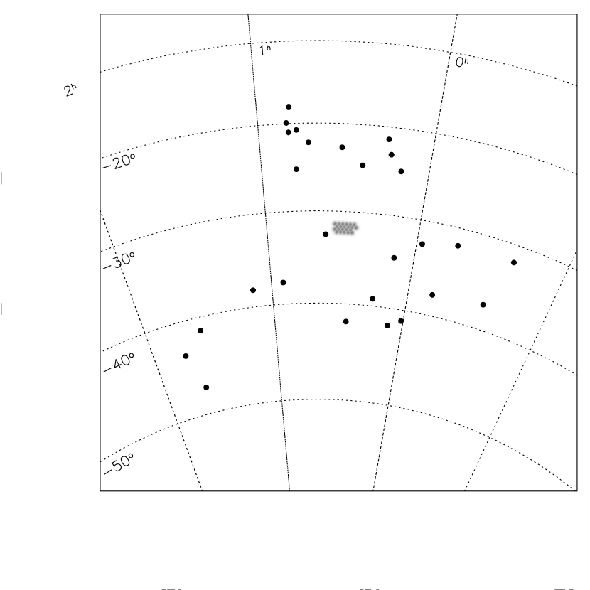
Figure 2: The observed grid on the sky of the Scl survey. Observed pointings are indicated by grey circles. Known galaxies are indicated by black points.

The individual pointings were gridded in data cubes using the same pixel size as the Cen cubes (i.e. $16^{\prime\prime}\times 16^{\prime\prime}\times 2$ km s^-1). The final cubes measured $256\times 256\times 410$ pixels, with the velocity axis running from $-310$ to 530 km s^-1. The synthesized beam size is $57^{\prime\prime}\times 29^{\prime\prime}$. The average noise per 2 km s^-1 channel was 10.2 (15.5) mJy for pointings A1-D4 (E1-F2). The column density sensitivity ($5\sigma$) for each 2 $\rm km\,s^{-1}$ channel is $7(10)\times 10^{19}$ cm^-2 or $1.5(2.3)\times 10^{20}$ after smoothing to 10 $\rm km\,s^{-1}$.

4 Analysis

4.1 Centaurus

4.1.1 Known Objects

In a number of fields previously catalogued objects were present within a $30^{\prime}$ radius of the field center and within the $0-1700$ km s^-1 velocity range. These fields are indicated with an asterisk in Table 1. These objects are listed in Table 2 along with their parameters as derived from the HIPASS data base.

A fair fraction could however not be retrieved from the ATCA data. These were usually objects that were far from the field center, where primary beam attenuation makes their signal too weak to retrieve. In total, four objects were detected. We list their parameters as derived from the ATCA data in Table 2 as well. Figure 3 shows integrated column density maps and spectra of three of the four detections (we do not show the M83 data: these are severely affected by missing spacing problems).

The two galaxies with H i masses of a few times $10^{8}$ $M_{\odot}$ are easily detected. The observation of IC 4316 with an H i mass of $3\cdot 10^{7}$ $M_{\odot}$ is almost at the limit of what the eye can see in the data. IC 4316 is $\sim 17^{\prime}$ from the pointing center and primary beam attenuation has reduced the signal to $\sim 0.55$ of the value it would have in the pointing center. As the velocity width of IC 4316 is $\sim 40$ km s^-1, it follows that the minimum H i mass that we could detect at the pointing center would be $\sim 8\times 10^{6}$ $M_{\odot}$ for a 20 $\rm km\,s^{-1}$-wide profile. Optimal smoothing would improve this limit by a factor of a few, bringing us close to the theoretical limit of the data. We will return to this after discussing the blind search.

Table 1: Positions Field Centers

Name	$\alpha(2000.0)$	$\delta(2000.0)$	$\sigma$ (mJy)
Centaurus
A1	13:32:24.00	-27:51:30.00	10.6
A2	13:37:00.00	-27:51:30.00	10.4 *
A3	13:37:00.00	-28:51:30.00	10.5 *
A4	13:32:24.00	-28:51:30.00	10.3
B1	13:41:36.00	-27:51:30.00	10.3
B2	13:46:12.00	-27:51:30.00	10.0
B3	13:46:12.00	-28:51:30.00	10.3
B4	13:41:36.00	-28:51:30.00	10.0 *
C1	13:32:24.00	-29:51:30.00	11.0
C2	13:37:00.00	-29:51:30.00	10.7 *
C3	13:37:00.00	-30:51:30.00	11.1 *
C4	13:32:24.00	-30:51:30.00	10.6
D1	13:41:36.00	-29:51:30.00	10.2 *
D2	13:46:12.00	-29:51:30.00	9.8
D3	13:46:12.00	-30:51:30.00	10.1
D4	13:41:36.00	-30:51:30.00	9.8
E1	13:32:24.00	-31:51:30.00	10.3
E2	13:37:00.00	-31:51:30.00	10.0
E3	13:37:00.00	-32:51:30.00	10.3
E4	13:32:24.00	-32:51:30.00	10.1
F1	13:41:36.00	-31:51:30.00	10.2 *
F2	13:46:12.00	-31:51:30.00	10.1
F3	13:46:12.00	-32:51:30.00	10.3
F4	13:41:36.00	-32:51:30.00	10.1
G1	13:32:24.00	-33:51:30.00	11.5
G2	13:37:00.00	-33:51:30.00	11.2
G3	13:37:00.00	-34:51:30.00	11.1
G4	13:32:24.00	-34:51:30.00	10.9
H1	13:41:36.00	-33:51:30.00	10.4
H2	13:46:12.00	-33:51:30.00	10.0
H3	13:46:12.00	-34:51:30.00	10.2
H4	13:41:36.00	-34:51:30.00	10.0
I1	13:32:24.00	-35:51:30.00	9.9
I2	13:37:00.00	-35:51:30.00	9.5
I3	13:37:00.00	-36:51:30.00	9.7
I4	13:32:24.00	-36:51:30.00	9.6
Sculptor
A1	0:33:00.24	-31:25:58.80	12.5
A2	0:32:15.12	-31:43:01.20	12.7
A3	0:30:44.88	-31:43:01.20	12.7
A4	0:31:30.00	-31:25:58.80	13.0
B1	0:30:00.00	-31:25:58.80	13.9
B2	0:29:14.88	-31:43:01.20	14.3
B3	0:27:44.64	-31:43:01.20	14.2
B4	0:28:29.76	-31:25:58.80	14.5
C1	0:26:59.76	-31:25:58.80	10.5
C2	0:26:14.64	-31:43:01.20	10.6
C3	0:24:44.40	-31:43:01.20	10.6
C4	0:25:29.52	-31:25:58.80	10.6
D1	0:33:00.24	-32:00:00.00	10.5
D2	0:32:15.12	-32:16:58.80	10.5
D3	0:30:44.88	-32:16:58.80	10.6
D4	0:31:30.00	-32:00:00.00	10.7
E1	0:30:00.00	-32:00:00.00	15.3
E2	0:29:14.88	-32:16:58.80	15.3
E3	0:27:44.64	-32:16:58.80	15.4
E4	0:28:29.76	-32:00:00.00	15.8
F1	0:26:59.76	-32:16:58.80	15.7
F2	0:26:14.64	-32:00:00.00	15.5

Table 2: Known galaxies in survey volume

Field	Name	$\alpha$ (2000.0)	$\delta$ (2000.0)	$V_{hel}$	$S$	${W_{20}}$	$\log M_{HI}$	$S$	${W_{20}}$	$R$	Notes
					ATCA			HIPASS
(1)	(2)	(3)	(4)	(5)	(6)	(7)	(8)	(9)	(10)	(11)	(12)
A2	ESO 444- G 084	13h37m20.1s	–28d02m46s	583	210.3	75	8.78	223.8	75	12.1
A3	UGCA 365	13h36m30.7s	–29d14m11s	577	–	–	–	177.0	52	23.6
B4	IC 4316	13h40m18.1s	–28d53m41s	577	11.5	43	7.51	$\sim 16.0$	40	17.2
C2	M83	13h37m00.8s	–29d51m59s	(516)	detected			detected		0
C2	[KK98] 208	13h36m35.5s	–29d34m17s	(381)	–	–	–	–	–	18.0	c
C2	MCG -05-32-042	13h35m07.9s	–30d07m05s	(300)	–	–	–	–	–	28.9	b
C3	ESO 444- G 082	13h37m07.3s	–30d58m59s	(526)	–	–	–	–	–	7.6	b
D1	NGC 5264	13h41m36.9s	–29d54m50s	482	152.1	44	8.64	265.1	52	3.3
F1	ESO 445- G 007	13h40m20.9s	–31d42m04s	1659	–	–	–	315.6	100	9.0	a
F1	NGC 5253	13h39m55.9s	–31d38m24s	407	–	–	–	522.4	104	25.0

Notes: (1) Field ID. (2) Galaxy identification. (3) Right Ascension (2000.0). (4) Declination (2000.0). (5) Heliocentric velocity. ATCA used where available, else HIPASS value. Value between brackets denotes catalog value. (6) Total flux ATCA observation in Jy km s^-1. (7) ATCA velocity width at 20% level. (8) Logarithmic ATCA H i mass. (9) Total flux HIPASS observation in Jy km s^-1. (10) HIPASS velocity width at 20% level. (11) Distance in arcmin to nearest field center. (12) Additional notes: (a) not detected: edge of band (b) not detected in HIPASS (c) confused with M83 in HIPASS

Figure 3: Integrated HI column density maps and integrated spectra of the detected known galaxies (M83 is not displayed here). Left: ESO 444-G084. Center: IC 4316. Right: N5264. Top row shows zeroth-moment maps. Contour levels are: [ESO 44-G084, left]: (1, 3, 5, 7, 9, 11)$\times 10^{20}$ cm^-2; [IC 4316, center]: (0.5, 1, 1.5, 2)$\times 10^{20}$ cm^-2; [N5264, right]: (1, 2, 3, 4, 5, 6, 7, 8)$\times 10^{20}$ cm^-2. Bottom row shows the integrated spectra. The spectrum of IC 4316 (center) has been hanning-smoothed.

4.1.2 Blind search

Method

The cubes were searched using an automatic search program in order to avoid any human biasses. Our proceedure extracts a spectrum at each spatial pixel and hanning smoothes it. A heavily smoothed (75 pixel boxcar) version of the spectrum is then subtracted to remove baseline ripple and other large-scale variations. This inevitably loses very wide profiles, but these observations are tuned to look for narrow signals. The difference spectrum is then searched for significant signals at different velocity resolutions. The spectra were searched at their original resolution and after smoothing with 3, 5, 9, and 15 pixel (6, 10, 18, 30 km s^-1) boxcars (one velocity pixel is 2 km s^-1). The first 30 and the last 50 channels were not searched as bandpass effects cause the noise there to be higher. The effective search range is therefore 192 - 1600 km s^-1. Signal due to the known galaxies was also removed prior to the automated search.

We decided to place our cut-off at the $5\sigma$ level. At this significance level the number of false detections expected due to Gaussian statistics is still managable: in each cube we expect to find $\sim 13$ noise pixels with values $>5\sigma$ (and a similar number with values $<-5\sigma$). At the $4\sigma$ level we would expect $\sim 1400$ false noise signals per cube, which is clearly unfeasible.

The actual detection process is a two-step one. Due to the large amount of data which must be inspected at four velocity resolutions, the computation speed is I/O limited. Our algorithm reads the datacube only once, one spectrum at a time, but the proceedure both (1) keeps a table of all signals with an absolute value $>4.5\sigma$ at any resolution evaluated relative to the noise level measured for each spectrum, and (2) accumulates the necessary statistical information to compute the noise level for each frequency plane in the cube. Each velocity range (frequency channel) might be corrupted by narrow RFI that would raise the noise level in certain individual planes in the cube. This permits a second pass through the list of tentative $>4.5\sigma$ detections to determine whether they are significant relative to the noise level in the velocity place where they were identified. Only the signals that made the $5\sigma$ cut at one or more velocity resolutions on the second pass were retained. This process was applied at all velocity resolutions with only one pass through the entire dataset.

To analyze the data at lower spatial resolution, we also applied the full detection algorithm to a new set of spatially smoothed cubes.

The output is a set of lists of positions with absolute flux values $>5\sigma$ for each velocity resolution. Obviously, there will be many cases where a signal is detected at multiple velocity resolutions. We have therefore also produced a list where all double or multiple detections (defined as $|\Delta R|<2$ pixels [32^′′] and $|\Delta V|<3$ pixels [6 km s^-1]) have been removed. We will refer to these as “double detections” or “doubles”.

For comparison, with this method IC 4316 is detected at the 8.0$\sigma$ level at the 15 channel (30 $\rm km\,s^{-1}$) resolution, at the $7.1\sigma$ level for 9 channels (18 $\rm km\,s^{-1}$), at $6.3\sigma$ for 5 channels (10 $\rm km\,s^{-1}$), at $5.6\sigma$ for 3 channels (6 $\rm km\,s^{-1}$) and at 5.0$\sigma$ at full spectral resolution (2 $\rm km\,s^{-1}$). It should be kept in mind that IC 4316 is located $17^{\prime}$ away from the pointing center. Had it actually been observed in the center of the field, then all significances would have been twice as high.

Results

In the absence of real signal and the presence of Gaussian noise we expect each cube to contain an equal number of “detections” with values above $5\sigma$ and below $-5\sigma$. For theoretical Gaussian noise there ought to be $\sim 26$ such pixels (13 positive and 13 negative) in each full-resolution cube, although counting statistics and the fact that we expect real data to have a slightly non-Gaussian noise distribution, means that the actual number of detections may vary a little.

Fig 4 plots the number of positive detections in each cube versus the number of negative ones. In the absence of any real signal we expect an equal number of cubes to have a positive and a negative excess. This is clearly the case for the Cen data (within the uncertainties mentioned before).

Table 3 summarizes the results. There is no clear evidence that the Cen data cubes contain anything more than noise at the $>5\sigma$ level.

Figure 4: Number of positive $>5\sigma$ detections versus number of negative $<-5\sigma$ detections in the Centaurus data. Each point represents one data cube. Different panels show different velocity resolution. Panel at the bottom-right combines all velocity resolutions but double detections have been removed.

Table 3: Positive and Negative Detections

	Number of cubes with
Resolution	pos $>$ neg	pos $=$ neg	pos $<$ neg
Centaurus
1 channel	19	1	16
3 channels	19	1	16
5 channels	18	2	16
9 channels	16	1	19
15 channels	17	5	14
no doubles	16	3	17
Sculptor
1 channel	7	2	13
3 channels	8	2	12
5 channels	7	4	11
9 channels	6	8	8
15 channels	1	18	3
no doubles	6	3	13

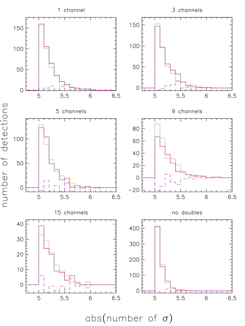
Figure 5: The distribution of the number of detections $>5\sigma$ versus the absolute values of their significance in the Centaurus data. The full lines represent the positive detections, the dotted lines the negative detections and the dashed lines the difference histogram. Different panels show different velocity resolution. Panel at the bottom-right combines all velocity resolutions but double detections have been removed.

A different way of looking at the results is to compare histograms of the peak flux distributions of the “detections.” This is done in Fig. 5, for each velocity resolution separately, and for the case where double detections have been removed. The positive and negative distributions are within their Poisson-errors indistinghuishable. Again we see no evidence for the presence of real objects in the data.

4.1.3 Spatial Smoothing

The beam size of $65^{\prime\prime}\times 43^{\prime\prime}$ is optimized to detect objects of $\sim 1$ kpc size at the distance of the Cen A group. In an attempt to find more extended objects we have smoothed the data by a factor of 5 spatially, resulting in a beam size of $325^{\prime\prime}\times 215^{\prime\prime}$ (this is roughly the maximum scale structure that the interferometer configuration that we have used is able to detect). We performed a similar blind search on the spatially smoothed data, but found no new $>5\sigma$ objects. The noise in the smoothed maps is 30 mJy, which for a channel separation of 2 $\rm km\,s^{-1}$, translates in a $5\sigma$ column density of $4.8\cdot 10^{18}$ cm^-2. After smoothing to 10 $\rm km\,s^{-1}$, the column density limit is $1.1\cdot 10^{19}$ cm^-2.

4.2 Sculptor

4.2.1 Known objects

In contrast with the Cen survey, there were no known extragalactic objects present in the survey area. We did detect an extended HVC centered at $00^{h}25^{m}24^{s},-31^{\circ}37^{m}57^{s}$, $v=-70$ km s^-1. This HVC is prominently visible in the HIPASS data. In most cubes a bright very narrow linewidth feature ($\sim 5$ km s^-1), presumably Galactic emission, is present at $v=+4$ km s^-1. These features were subsequently blanked in the data in order to facilitate the blind search.

4.2.2 Blind search

The Scl data cubes were searched in the same way as the Cen cubes. Fig. 6 shows for each velocity resolution separately the number of $>5\sigma$ detections plotted agains the number of $<-5\sigma$ detections. Table 3 summarizes these results. As with Cen there is no evidence for an excess of positive detections. There is a hint of an excess of negative detections, however this is at most a $\sim 1.5\sigma$ difference. The excess negative detections occur in a narrow velocity range adjoining the (blanked out) Galactic emission, and are therefore most likely artefacts caused by the relatively strong Milky Way emission. Figure 7 shows the noise histograms for both positive and negative signals. As with Centaurus we find no evidence for the presence of anything other than noise.

Figure 6: Number of positive $>5\sigma$ detections versus number of negative $<-5\sigma$ detections in the Sculptor data. Each point represents one data cube. Different panels show different velocity resolution. Panel at the bottom-right combines all velocity resolutions but double detections (at one or more smoothings) have been removed.

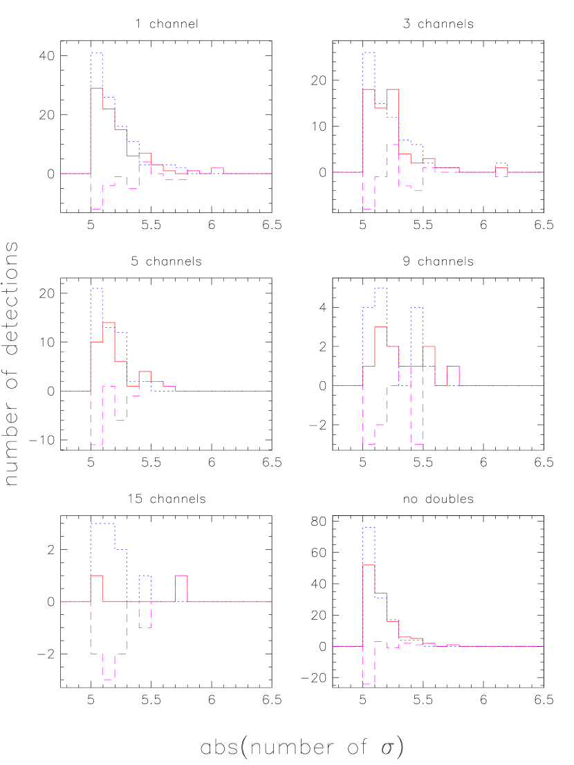
Figure 7: The distribution of the number of detections $>5\sigma$ versus the absolute values of their significance in the Sculptor data. The full lines represent the positive detections, the dotted lines the negative detections and the dashed lines the difference histogram. Different panels show different velocity resolution. Panel at the bottom-right combines all velocity resolutions but double detections (at one or more velocity resolutions) have been removed.

4.2.3 Spatial Smoothing

We smoothed the data to one-fifth of its original spatial resolution (resulting beam $285^{\prime\prime}\times 145^{\prime\prime}$). Apart from the aforementioned HVC and the Galactic signal we did not detect any additional detections with a significance $>5\sigma$. For pointings A1-D4 (E1-F4) the noise was 47 (61) mJy, which for a channel spacing of 2 $\rm km\,s^{-1}$, translates in a $5\sigma$ column density sensitivity of $1.3\ (1.6)\cdot 10^{19}$ cm^-2, and after smoothing to 10 $\rm km\,s^{-1}$to a column density sensitivity of $2.8\ (3.7)\cdot 10^{19}$ cm^-2.

5 Discussion

Figure 8: Space densities of objects as a function of H i mass in the Centaurus and Sculptor groups. The solid curve indicates an HiMF with a faint-end slope of $\alpha=-1.2$ (Zwaan et al. 1997), scaled vertically by a factor 300 to compensate for the overdensity in the groups. The dashed lines represent the reciprocals of the surveyed volumes within the group, for objects with velocity widths of 2, 6, 10, 18, and 30 $\rm km\,s^{-1}$ (from left to right). Detections are expected where the HiMF exceeds these lines. Since no new objects were detected in this survey, steep faint-end slopes of the HiMF can be excluded.

Fig. 8 shows the space density of galaxies in the two surveyed groups, in combination with the sensitivity of the surveys. The solid dots represent the space density of known group members with measured H i masses (Côté et al. 1997), which are calculated by dividing the number of galaxies per 0.5 dex bin, by the total volume of the group. For the group radii we adopt the values $R=0.64$ Mpc for Cen A (van den Bergh 2000) and $R=0.66$ Mpc for Sculptor (Freeman 1997).

We estimate a mean overdensity of the groups by vertically scaling the Schechter fit to the field H i mass function from Zwaan et al. (1997) so as to fit the points in Fig. 8. Using this method we arrive at an overdensity in the two groups of 300 times the cosmic mean. This number should be regarded as a rough indication of the groups’ overdensity because the calculation is heavily dependent on the definition of the groups’ boundaries. The calculation assumes that the groups are spherical while the actual shape of the groups are more complicated. This is especially true for Cen A as can be seen from Fig. 1, but possibly also for Sculptor (Jerjen et al. 1998). Furthermore, due to substructure in the groups, the actual overdensity is a strong function of the position in the groups. For the conclusions reached in this paper, the value of the overdensity is however not crucial.

The dashed lines in Fig. 8 show the reciprocal of the surveyed volumes for different assumed velocity widths of H i clouds or galaxies. They are calculated for optimal spectral smoothing for velocity widths of 2, 6, 10, 18, and 30 $\rm km\,s^{-1}$ (from left to right). The shape of the curves is determined by the (approximately) Gaussian primary beam of the survey. Larger volumes are searched for higher mass galaxies since these can be detected out to larger distances from the centre of the primary beam. The curves level off at H i masses of approximately $10^{8}M_{\odot}$, because we assume that no detections can be made at separations larger that 35 arcmin (equal to the FWHM) from the centre of the primary beam.

From the information presented in Fig. 8 it is now trivial to calculate how many detection the survey should have turned up assuming different shapes of the H i mass function. This number can be evaluated by taking the integral over H i mass function multiplied by the survey volume. Assuming the HiMF as presented in Fig. 8, and a velocity width of 6 $\rm km\,s^{-1}$, the survey should have detected $2.6$ galaxies. This number drops to 1.8 and 1.7 for velocity widths of 30 and 50 $\rm km\,s^{-1}$. More detection are expected if the HiMF would show an upturn below $M_{\rm HI}=10^{7.5}M_{\odot}$, as has been proposed by Schneider, Spitzak & Rosenberg (1998). If the faint-end of the HIMF would have a steep slope with $\alpha=-1.5$ below $M_{\rm HI}=10^{7.5}M_{\odot}$, the expected number of detections would rise to 5.3, 2.4 and 2.1 using velocity widths of 6, 30 and 50 $\rm km\,s^{-1}$. Clearly, even steeper extensions of the HiMF are excluded by our present survey.

The null-result of this group survey can be used to place tight constraints on the space density of small H i clouds in galaxy groups. Fig. 9 shows the combined constraint on the H i mass of intragroup clouds and the space density of clouds. The lines show the 95% confidence levels on the existence of cloud populations. These lines are calculated assuming Poisson statistics and the fact that no new clouds were detected. Regions of parameter space above each line are excluded by our survey.

Figure 9: 95% confidence upper limits to the space density of H i clouds for objects with velocity widths of 2, 10, and 30 $\rm km\,s^{-1}$. Also shown as a dashed curve is the upper limit to the space density of H i clouds derived by Zwaan (2001) by means of Arecibo survey in five galaxy groups. The limits set by the present survey are stricter, but only apply to clouds with column densities $N_{\rm HI}>10^{20}\rm cm^{-2}$.

For comparison, we also show the 95% confidence upper limits on cloud populations as calculated by Zwaan (2001) by means of a pointed Arecibo survey in five galaxy groups. The limits on intragroup H i clouds from the present survey are slightly stricter than those from Zwaan (2001), but care should be taken with the interpretation of the results. The surface brightness sensitivity of the Arecibo group survey was much better, resulting in very low detectable H i column densities of $1.0\times 10^{18}\rm cm^{-2}$ ($5\sigma$) per 16 $\rm km\,s^{-1}$ for gas filling the beam. The full resolution H i column density sensitivity of the present ATCA survey is $1.0\times 10^{20}\rm cm^{-2}$ ($5\sigma$) per 10 $\rm km\,s^{-1}$. The two surveys are therefore sensitive to different populations of H i clouds, the Arecibo survey to lower column densities, the ATCA survey to lower H i masses.

The beam area of the smoothed cubes is $\sim 25$ times larger than in the original resolution cubes, and the column density sensitivity is a factor of 10 better, so in principle the smoothed cubes could be used to constrain the density of more diffuse H i clouds, and would be suitable to assess the problem of extragalactic HVCs (Blitz et al. 1999). However, as our column density sensitivity and survey volume are less than those of the surveys by Zwaan & Briggs (2000) and Zwaan (2001), our limits are not as strong as the ones presented in those surveys.

Using the parameters of compact HVCs from Putman et al. (2002), we expect them to have sizes of approximately $2.5^{\prime}$ at the distance of the surveyed groups, and having peak column densities of $1.4\times 10^{19}\rm cm^{-2}$ over 35 $\rm km\,s^{-1}$. This means that most of the CHVCs in the groups would escape detection in the present survey.

In summary, the current survey supports the conclusion reached previously that HVCs are not objects with H i masses $\sim 10^{7}M_{\odot}$ distributed throughout galaxy groups, but does not improve on them.

6 Conclusions

One of the results of the CDM theory of formation of structure in the universe is that every galaxy group should be filled with a few hundred small mass halos. Optical surveys for these objects have only turned up $\sim$ 10% of the predicted numbers. If the density of the primordial H i in the satellites is sufficiently high to prevent ionization by the meta-galactic uv-background, they should be detectable in 21cm H i surveys. This motivated us to perform a sensitive 21cm search in two nearby galaxy groups: the Centaurus A and Sculptor groups.

We have used the Australian Telescope Compact Array to observe 36 fields in the Cen A group in the velocity range 192–1600 km s^-1 and 22 fields in the Sculptor region in the velocity range $-300$-500 km s^-1. The surveys are sensitive to H i masses down to a few times $10^{6}$ $M_{\odot}$, which is an improvement of a factor 10 on previous surveys. These surveys were tuned to pick up narrow profiles that might in single-dish surveys with a coarser velocity resolution have been confused with RFI.

We find no new detections, though observations of known galaxies show that we do indeed reach our theoretical mass limit. This null-result rules out faint HiMF slopes steeper than $\alpha=-1.5$ below $10^{7.5}\ M_{\odot}$ in these groups, and puts tight constraints on the occurence of compact H i clouds in other groups.

We have also searched the data for extended and diffuse H i clouds, and our null-detections support the results derived by e.g. Zwaan & Briggs (2000) and Zwaan (2001) that HVCs are not distributed in the intra-group environment on scales of 1 Mpc.

References

- Banks et al. (1999) Banks, G. D. et al. 1999, ApJ, 524, 612
- Barnes & de Blok (2001) Barnes, D.G., & de Blok, W.J.G., 2001, ApJ, in press
- Barnes et al. (2001) Barnes, D.G., et al., 2001, MNRAS, 322, 468
- Blitz et al. (1999) Blitz, L., Spergel, D.N., Teuben, P.J., Hartmann, D., Burton, W.B., 1999, ApJ, 514, 818
- Braun & Burton (2001) Braun, R., Burton, W.B., 2001, A&A, 375, 219
- Braun & Burton (1999) Braun, R., Burton, W.B., 1999, A&A, 341, 437
- Côté et al. (1997) Côté, S., Freeman, K. C., Carignan, C., & Quinn, P. J. 1997, AJ, 114, 1313
- Côté, Carignan, & Freeman (2000) Côté, S. ;., Carignan, C., & Freeman, K. C. 2000, AJ, 120, 3027
- Dahlem et al. (2001) Dahlem, M., Ehle, M., Ryder, S.D., 2001, A&A, 373, 485
- de Blok et al. (2001b) de Blok, W.J.G., McGaugh, S.S., Bosma, A., Rubin, V.C., 2001, ApJL, 552, L23
- Freeman (1997) Freeman, K.C., 1997, PASA, 14, 4
- Haynes & Roberts (1979) Haynes, M.P., Roberts, M.S. 1979, ApJ, 227, 767
- Jerjen et al. (1998) Jerjen, H., Freeman, K.C., Binggeli, B., 1998, AJ, 116, 2837
- Jerjen et al. (2000) Jerjen, H., Binggeli, B., Freeman, K.C., 2000, AJ, 119, 166
- Kilborn et al. (2000) Kilborn, V.A., et al., 2000, AJ, 120,1342
- Klypin et al. (1999) Klypin, A.A., Kravtsov, A.V., Valenzuela, O., Prada, F., 1999, ApJ, 522, 82
- Moore et al. (1999a) Moore, B., Quinn, T., Governato, F., Stadel, J., Lake, G., 1999, MNRAS, 310, 1147
- Moore et al. (1999b) Moore, B., et al., ApJL, 524, 19
- Navarro, Frenk & White (1996) Navarro, J.F., Frenk, C.S., White, S.D.M. 1996, ApJ, 462, 563
- Navarro, Frenk & White (1997) Navarro, J.F., Frenk, C.S., & White, S.D.M. 1997, ApJ, 490, 493
- Putman et al. (2002) Putman, M., et al., 2001, AJ, in press
- Rosenberg & Schneider (2000) Rosenberg, J.L., Schneider, S.E., 2000, ApJS, 130, 177
- Schneider, Spitzak & Rosenberg (1998) Schneider, S.E., Spitzak, J.G., Rosenberg, J.L., 1998, ApJL, 507, L9
- van den Bergh (2000) van den Bergh, S., 2000, AJ, 119, 609
- Verheijen et al. (2000) Verheijen, M.A.W., Trentham, N., Tully, R.B., Zwaan, M.A. 2000, in “Mapping The Hidden Universe: The Universe Behind the Milky Way The Universe in HI”, eds. R.C. Kraan-Korteweg, P.A. Henning, H. Andernach, ASP Conf. Series 218, p 263
- Zwaan (2001) Zwaan, M.A., 2001, MNRAS, 325, 1142
- Zwaan & Briggs (2000) Zwaan, M.A., & Briggs, F.H. 2000, ApJL, 530, 61
- Zwaan et al. (1997) Zwaan, M.A., Briggs, F.H., Sprayberry, D., Sorar, E. 1997, ApJ, 490, 173