Searching for Pulsars in Close Binary Systems

We present a detailed mathematical analysis of the Fourier response of binary pulsar signals whose frequencies are modulated by circular orbital motion. The fluctuation power spectrum of such signals is found to be $\nu_{\rm orb}$-periodic over a compact frequency range, where $\nu_{\rm orb}$ denotes orbital frequency. Subsequently, we consider a wide range of binary systems with circular orbits and short orbital periods, and present a Partial Coherence Recovery Technique for searching for binary millisecond X-ray and radio pulsars. We use numerical simulations to investigate the detectability of pulsars in such systems with $P_{\rm orb}\raisebox{-1.29167pt}{\mbox{$\stackrel{{\scriptstyle<}}{{{}_{\sim}}}\,$}}6$ hours, using this technique and three widely used pulsar search methods. These simulations demonstrate that the Partial Coherence Recovery Technique is on average several times more sensitive at detecting pulsars in close binary systems when the data span is more than 2 orbital periods. The systems one may find using such a method can be used to improve the constraints on the coalescence rate of compact objects and they also represent those systems most likely to be detected with gravitational wave detectors such as LISA.

1 Introduction

The importance of binarity and the connection with the low-mass X-ray binaries (LMXBs) in the formation of millisecond pulsars (Alpar et al. 1982; Radhakrishnan & Srinivasan 1982) extends back to the discovery of the first millisecond pulsar (Backer et al. 1982). In the intervening years, a large number of binary millisecond radio pulsars and X-ray pulsars have been discovered (for recent reviews see Kramer et al. 2000). However, these tend to be either bright pulsars, members of wide binaries or to have low-mass companions. The remaining systems are more difficult to detect owing to large orbital accelerations which cause, via the time-dependent Doppler effect, the apparent pulse period to change significantly during long integrations. Compensating completely for this smearing of the pulsed signal is extremely computationally expensive as a large range of orbital parameters has to be searched.

Numerous authors have developed and used techniques to partially correct for this smearing, e.g. Middleditch & Priedhorsky (1986); Anderson et al. (1990); Wood et al. (1991); Ransom (1999). In 1990 Anderson et al.. Anderson et al. (1990) used a constant acceleration technique to successfully discover PSR 2127+11C in the globular cluster M15. Despite the success of this survey, it was not until recently that the true extent of the binary millisecond pulsar population that could be uncovered by using such techniques became apparent (Camilo et al. 2000; D’Amico et al. 2000; Ransom et al. 2000). However a whole possible population of rapidly rotating radio/X-ray pulsars in close binary systems still remains to be investigated as even the current best search strategies are not very sensitive to them. This population includes faint pulsars in similar type binaries, pulsars in tighter binaries and those with more massive companions.

Following the discovery of a large number of binary millisecond pulsars in the globular cluster 47Tuc (Camilo et al. 2000), Rasio, Pfahl & Rappaport (2000) tried to model this observed population. They find that a large number of neutron star - white dwarf binaries in even tighter orbits and possibly more massive companions than those already discovered should exist in 47Tuc. The existence of very short orbital period LMXBs such as 4U 1820-30 (Stella, White & Priedhorsky 1987), and millisecond pulsars with relatively massive companions, e.g. PSR B1744-24A (Lyne et al. 1990), also indicate that very short period binary millisecond pulsars should exist in globular clusters (Bisnovatyi-Kogan 1989; Ergma & Fedarova 1991). Furthermore, multi-frequency radio imaging of globular clusters has revealed several unidentified steep-spectrum radio sources whose variable flux-densities and spectral indexes suggest radio pulsars (Fruchter & Goss 1990; 2000). Subsequent pulsed searches (e.g. Lyne et al. 1990; D’Amico 1993; Biggs et al. 1994) have detected millisecond pulsars coincident with some of these point sources supporting the idea that the remainder are also pulsars which are so far undetected. Moreover, the number of pulsars detected in globular clusters is far less than the expected population based on the integrated flux density of the cores of some of the clusters. It has been argued that even bright pulsars could have been missed by previous searches due to Doppler smearing caused by the orbital motion in close binary systems, even though their radio emission remains detectable by interferometric observations. A further source of possible pulsar candidates are the subset of the EGRET unidentified $\gamma$-ray sources whose distribution above the Galactic disk has a scale height of about 2 kpc (Grenier 2001). These sources have so far evaded detection as radio pulsars and this may be because they are members of close binaries.

The physics of gravitation in such extreme systems has recently received growing attention because such binary systems will be the most common known continuous sources of gravitational radiation for gravitational wave detectors. The Laser Interferometer Space Antenna (LISA) will be especially sensitive to compact neutron star binaries with ultra-short orbital periods and large ($\stackrel{{\scriptstyle>}}{{{}_{\sim}}}\,$ 0.5 M_⊙) companion masses (Benacquista, Portegies Zwart & Rasio 2000). Detecting and studying pulsed radio or X-ray emission from the neutron stars in these systems will provide better constraints on the binary parameters and therefore be of paramount importance in helping to understand the gravitational wave emission (Dhurandhar & vecchio 2000). Discovering such systems is further motivated by improving the constraints on the coalescence rate of compact objects which remains difficult to estimate. Therefore, both theoretical predictions and observational evidence strongly encourage searching for highly accelerated millisecond pulsars in globular clusters.

Thus motivated, we present here a detailed mathematical analysis of the Fourier response of a radio/X-ray binary pulsar signal. We then discuss the sensitivity of three widely used search techniques applied to a range of binary systems. In Sec. 5, we present a complete description of our Partial Coherence Recovery Technique, which is based on the Phase Modulation Searching method first discussed by Ransom (Ransom 1999). We also discuss the computational cost of the method, how to estimate detection levels and how to derive all the binary parameters directly from the Fourier signature of the binary. Finally we compare the sensitivity of these different search techniques and show that our method is not only computationally very efficient but also significantly more sensitive to very tight binaries.

A list of the main symbols we use in this paper accompanied by a short description can be found in Appendix A.

2 Pulsar signal

Consider a pulsar with a pulse frequency $\nu_{\rm psr}$, whose distance from the observer $d(t)$ is changing with time $t$. The pulsar signal $s(t)$ emitted at time $t$ is received by the observer at time $t+d(t)/{\rm c}$, and can be represented by its harmonic decomposition

$$s(t)=\sum_{n=0}^{\infty}s_{n}(t)\hskip 7.22743pt,\hskip 7.22743pts_{n}(t)=A_{n}(t)\,e^{\,2\pi jn\nu_{\rm psr}\,\left[t+d(t)/{\rm c}\right]}$$ (1)

where $A_{n}(t)$ is the complex amplitude of the $n^{\rm th}$ harmonic, c the velocity of light and $j=\sqrt{-1}$. We consider binary systems in circular orbits, for which the projected distance to the observer is

$$d(t)=[a_{1}\sin(i)]\cos\left(2\pi\nu_{\rm orb}t+{\rm\phi_{orb}}\right)\,+\,{\rm Constant}$$ (2)

where $a_{1}$ is the pulsar’s orbital radius, $i$ the orbital inclination in radians, $\nu_{\rm orb}$ the orbital frequency and $\phi_{\rm orb}$ the initial orbital phase measured from superior conjunction of the pulsar. For simplicity, we shall take Constant = 0. Expanding Eq. (2) in Eq. (1) yields

$$s_{n}(t)=A_{n}(t)\,e^{\,2\pi jn\nu_{\rm psr}t}\,e^{\,j\varphi_{n}\cos\left(2\pi\nu_{\rm orb}t+\mathrm{\phi_{orb}}\right)}$$ (3)

where $\varphi_{n}=2\pi n\nu_{\rm psr}\left[a_{1}\sin(i)/{\rm c}\right]$ represents half the phase rotation in radians experienced by the $n^{\rm th}$ harmonic of the pulsar signal during the orbit. Since the signal $s_{n}(t)$ is the $n^{\rm th}$ harmonic of the Fourier series decomposition, we shall study its Fourier response.

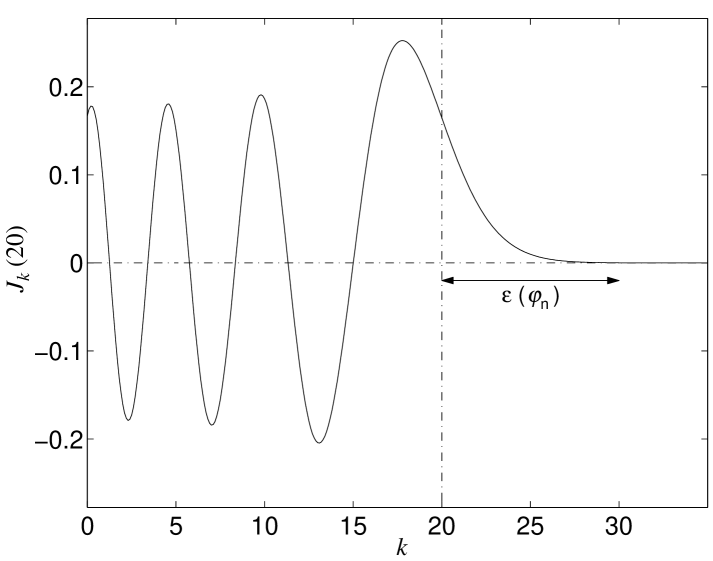
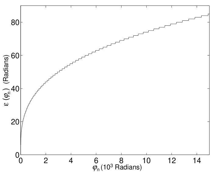
Figure 1: (a) left: $J_{k}(\varphi_{n})$ with $\varphi_{n}=20$. We plot $k\in{\mathbb{R}}$ whereas in reality $k\in{\mathbb{N}}$. The Fourier response slightly extends beyond the amplitude of the phase modulation as $\varepsilon(\varphi_{n})\neq 0$. (b) right: in the general case, we plot $\varepsilon(\varphi_{n})$ as a function of $\varphi_{n}$.

3 Fourier analysis

We denote the Fourier response of any function $\Psi$ by $\tilde{\Psi}$ and define it by $\tilde{\Psi}(\nu)={\cal F}[\Psi(t)](\nu)$ where $\nu$ indicates the frequency and ${\cal F}$ the Fourier Transform operator. As regards notations, Int[ ] shall define the integer part of and Frac[ ] the fractional part of. Henceforth for consistency with future notations, we call T-space what is usually referred to as the time domain.

In an ideal case, the complex amplitude $A_{n}(t)\equiv A_{n}$, and the pulsar signal is a periodic function. However, in most astrophysical cases the periodicity of the signal is violated because

1. The pulsed signal strength might vary during the observation due to eclipses, interstellar scintillation and observational windowing.

2. The pulsed signal could be modulated by stochastic or deterministic processes such as radio pulsar nulling, drifting subpulses or microstructure.

The latter effects are not so important because the average pulse profile of radio pulsars is known to remain stable within the observing window. Nevertheless in practice, $A_{n}(t)$ is a function of time but the modulation itself remains to a large extent a priori unknown to the observer.

3.1 Continuous Fourier response

Let $\xi_{n}(t)=e^{\,j\varphi_{n}\cos\left(2\pi\nu_{\rm orb}t+\mathrm{\phi_{orb}}\right)}$ define the phase rotation factor of Eq. (3) and $W(t)$ a real window function of finite duration. For an observation constrained by a window $W(t)$, Eq. (3) can be rewritten as

$$s_{n}(t)=A_{n}(t)\,\xi_{n}(t)\,W(t)\,e^{\,2\pi jn\nu_{\rm psr}t}\,.$$ (4)

According to Fourier theory and by virtue of the shift theorem,

$$\tilde{s}_{n}(\nu)=\tilde{A}_{n}(\nu)*\left[\tilde{\xi}_{n}(\nu)*\tilde{W}(\nu-n\nu_{\rm psr})\right]$$ (5)

where $*$ denotes the convolution operator. As we aim to study the Fourier response of the pulsating signal, we shall start with the calculation of $\tilde{\xi}_{n}(\nu)$. By definition,

$$\tilde{\xi}_{n}(\nu)=\int_{-\infty}^{\infty}\xi_{n}(t)\,e^{\,-2\pi j\nu t}\,\mathrm{d}t\,.$$ (6)

The integration of Eq. (6) requires the substitution of $\xi_{n}(t)$ by its series expansion given by (see Appendix B)

$$\xi_{n}(t)=\sum_{k=-\infty}^{\infty}J_{k}(\varphi_{n})\,e^{\,jk[\phi_{\rm orb}+\pi/2]}\,e^{\,2\pi jk\nu_{\rm orb}t}$$ (7)

where $J_{k}$ are Bessel Functions of the First Kind of integer order and $k\in{\mathbb{N}}$ (see also Middleditch 1981). Combining Eqs. (6) and (7) yields

$$\tilde{\xi}_{n}(\nu)=\sum_{k=-\infty}^{\infty}\left[J_{k}(\varphi_{n})\,e^{\,jk[\phi_{\rm orb}+\pi/2]}\right]\,\delta(\nu-k\,\nu_{\rm orb})$$ (8)

where $\delta$ denotes Dirac’s delta function. This convolution greatly simplifies Eq. (8) into

$$\tilde{\xi}_{n}(\nu)=\left\{\begin{array}[]{cl}J_{k}(\varphi_{n})\,e^{\,jk[\phi_{\rm orb}+\pi/2]}&\hskip 7.22743pt\nu=k\,\nu_{\rm orb}\\ 0&\hskip 7.22743pt\mathrm{otherwise}\end{array}\right.\,.$$ (9)

In the ideal case of an infinite and continuous observation, $\tilde{\xi}_{n}(\nu)$ represents the Fourier response of the $n^{\rm th}$ harmonic of a signal of constant amplitude emitted by a pulsar whose phase is modulated by circular orbital motion. Following Eq. (5), $\tilde{\xi}_{n}(\nu)$ is defined in Eq. (9) relative to the $n^{\rm th}$ harmonic frequency taken as the origin of the frequency scale. Of particular interest is its power spectrum, defined by $P_{\xi,n}(\nu)=|\tilde{\xi}_{n}(\nu)|^{2}$. A number of important properties of $P_{\xi,n}$ are :

1. Periodicity

   $P_{\xi,n}$ is a periodic sequence with period $\nu_{\rm orb}$ whose amplitude is modulated by $J_{k}^{2}(\varphi_{n})$.

2. Compactness

   Since $k$ is an integer, $J_{-k}(\varphi_{n})=(-1)^{k}\,J_{k}(\varphi_{n})$ hence $P_{\xi,n}$ is symmetric with respect to $k=0$. Furthermore, $\exists\,\varepsilon(\varphi_{n})\;,\;\forall\,k>[\varphi_{n}+\varepsilon(\varphi_{n})]\;:$

   $$|J_{k}(\varphi_{n})|<\left|\frac{{\rm Max}[J_{k}(\varphi_{n})]_{k}}{1000}\right|$$

   (see Abramowitz & Stegun 1974 and Fig. 1(a)). As shown in Fig. 1(b), $\varepsilon(\varphi_{n})\ll\varphi_{n}$ so $J_{k}(\varphi_{n})$ only slightly extends beyond its argument. Therefore, $P_{\xi,n}$ is compact on the interval $I(\varphi_{n},\nu_{\rm orb})=[-{\rm E}(\varphi_{n})\,\nu_{\rm orb}\,{\rm;}\,{\rm E}(\varphi_{n})\,\nu_{\rm orb}]$ where ${\rm E}(\varphi_{n})\leavevmode\nobreak\ =\leavevmode\nobreak\ \varphi_{n}\leavevmode\nobreak\ +\leavevmode\nobreak\ \varepsilon(\varphi_{n})$ radians. Note that

   $$\varphi_{n}\,\nu_{\rm orb}=\frac{v_{\rm max}}{\rm c}\,n\,\nu_{\rm psr}$$ (10)

   where $v_{\rm max}$ denotes the maximum radial velocity of the pulsar. Thus, $\varphi_{n}\,\nu_{\rm orb}$ represents the amplitude of the Doppler shift experienced by the $n^{\rm th}$ harmonic of the pulsar. $P_{\xi,n}$ is a comb of $\sim 2\,\varphi_{n}$ sidebands with a spacing of $\nu_{\rm orb}$.

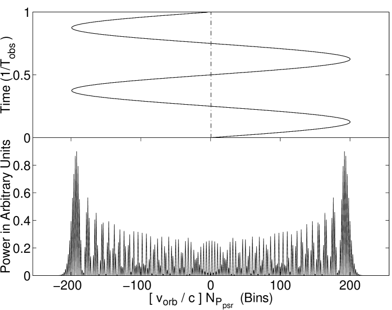
Figure 2: Top : pulsar radial velocity in units of Fourier frequency bins (v_orb denotes the radial velocity of the pulsar). Bottom : power spectrum of the 1^st harmonic shifted back to the origin of the frequency scale ($P_{\zeta,1}$) in arbitrary units. Here, $\varphi_{1}=100$, $N_{P_{\rm orb}}=2.0$ and $\phi_{orb}=0$. The response is symmetric because the pulsar signal is periodic in the observing window and $N_{P_{\rm orb}}$ is an integer.

3.2 Discrete Fourier response

By necessity, any observed signal is of finite extent. The extent may be adjustable and selectable, but must be finite. Processing a finite-duration observation by estimating its complex spectrum directly from the Fourier Transform encounters many difficulties which make a binary pulsar’s Fourier response more complicated.

3.2.1 Frequency sampling

In practice, we define

$$\nu\equiv\nu_{\ell}\hskip 7.22743pt{\rm and}\hskip 7.22743pt\nu_{\ell}=\frac{\ell}{T_{\rm obs}}\,,\hskip 7.22743pt\ell\in{\mathbb{N}}_{\,[0,N/2-1]}$$

where $T_{\rm obs}$ is the observing time, $N$ the number of equally spaced sampling points in the data set and $\ell$ the bin number in the Fourier spectrum. Following Sec. 3.1, we define $\tilde{\zeta}_{n}(\ell)$ as the discrete Fourier response of the $n^{\rm th}$ harmonic of a signal of constant amplitude emitted by a pulsar whose phase is modulated by circular orbital motion. We also define its power spectrum $P_{\zeta,n}(\ell)=|\tilde{\zeta}_{n}(\ell)|^{2}$. Henceforth for convenience, various quantities such as orbital frequency $\nu_{\rm orb}$ will be expressed in units of Fourier bins instead of frequencies. Thus, $\nu_{\rm orb}$ can also be referred to as $N_{P_{\rm orb}}=\nu_{\rm orb}\,T_{\rm obs}$ in the context of a particular observation of length $T_{\rm obs}$. The previous results then imply that

1. $P_{\zeta,n}$ is a spiky $N_{P_{\rm orb}}$-periodic sequence with a modulated amplitude. The periodicity is now expressed in units of Fourier bins. Also note that

   $$\varphi_{n}\,N_{P_{\rm orb}}=\frac{v_{\rm max}}{\rm c}\,n\,N_{P_{\rm psr}}$$ (11)

   where $N_{P_{\rm psr}}=\nu_{\rm psr}\,T_{\rm obs}$ is the number of pulse periods in the observation.

2. The Fourier response $\tilde{\zeta}_{n}$ is compact on the interval $I(\varphi_{n},N_{P_{\rm orb}})$ about the $n^{\rm th}$ harmonic. It corresponds to the Doppler shift interval of the $n^{\rm th}$ harmonic of the pulsar signal expressed in units of Fourier bins and can be approximated by $2\,N_{P_{\rm orb}}\,\varphi_{n}$ (see Fig. 2).

A $N$-point Fourier Transform is elegant when the processing scheme is cast as a spectral decomposition in an $N$-dimensional orthogonal vector space. However, such remarkable efficiency is compromised in practice because the number of orbital periods and pulse periods contained in an observation are not integers.

3.2.2 Spectral leakage

From the continuum of possible frequencies $\nu$, only those which coincide with the basis of discrete frequencies $\nu_{\ell}$ will project onto a single complex vector in the Fourier spectrum. All other frequencies will exhibit non zero projections on the entire basis set. This is often referred to as spectral leakage and results from processing finite-duration signals whose frequencies are not periodic in the observation window $W$. This leakage can strongly degrade a signal’s Fourier response.

Multiplicative weighting windows can be used to minimize such an effect (Harris 1978). Such windows proved very useful for multiple-tone signal detection. However, they convey other intrinsic properties that make the detection of noisy signals difficult:

• The Equivalent Noise Bandwidth increases.

• The independent noise samples become correlated and the estimation of the probability density function of the noise consequently increases in complexity.

• If the windows are applied to overlapping partitions of the data sequence, the noise samples become even more correlated. The work load also increases.

Hence we compute the Fourier response given by the straight FFT of the data set. We can now rewrite Eq. (5) for the case of a discrete Fourier Transform as $\tilde{s}_{n}(\ell)=\tilde{A}_{n}(\ell)*[\tilde{\zeta}_{n}(\ell)*\delta(\ell-n\,N_{P_{\rm psr}})]$ where

$$\tilde{\zeta}_{n}(\ell)=\sum_{k=-{\rm Int}[E(\varphi)]}^{{\rm Int}[E(\varphi)]} \left[\rule{0.0pt}{14.22636pt}J_{k}(\varphi_{n})\,e^{\,jk[\phi_{orb}+\pi/2]}\,\times\right.$$ (12)

$$\left.\tilde{W}(\ell-k\,N_{P_{\rm orb}})\rule{0.0pt}{14.22636pt}\right]\,.$$

$\tilde{\zeta}_{n}$ can be calculated for virtually any window $W$ provided its Fourier response is known. In that sense, Eq. (12) represents the analytical solution to the problem of Fourier analysis of noiseless binary pulsar signals in the solar system barycentric frame. In practice, $W$ is defined by a Boxcar function whose Fourier response is given by

$$\tilde{W}_{B}(\ell)=T_{\rm obs}\,e^{\,-j\pi\ell}\,{\rm sinc}\,(\ell)\hskip 7.22743pt,\hskip 7.22743pt{\rm sinc}\,(\ell)=\frac{\sin\,(\pi\ell)}{\pi\ell}\,.$$ (13)

3.2.3 Computational cost

Obviously, $\tilde{\zeta}_{n}$ can be computed using Eq. (12). The sine, cosine and Bessel functions can be pre-computed and stored in static lookup tables. The computational cost of estimating $\tilde{\zeta}_{n}$ over its compact interval for the simple case of the Boxcar function amounts to $\sim$ $50\;N_{P_{\rm orb}}E(\varphi_{n})^{2}$ operations.

Alternatively, $\tilde{\zeta}_{n}$ can be evaluated numerically by computing a Fast Fourier Transform (FFT) of a simulated data set of length $K=4$^${\,{\rm Int}\left[\,\log_{2}I(\varphi_{n},N_{P_{\rm orb}})\,\right]}$ defined by

$$\zeta_{n}(k) = \exp\left[2\pi jn\left(\frac{K}{2}+\eta\right)\frac{k}{K}+\right.$$ (14)

$$\left.j\varphi_{n}\cos\left(2\pi N_{P_{\rm orb}}\frac{k}{K}+\phi_{\rm orb}\right)\right]$$

where $k\in[0\,{\rm;}\,K-1]$. The spectral leakage factor is defined by $\eta={\rm Min}[{\rm Frac}[\nu_{\rm psr}T_{\rm obs}],1-{\rm Frac}[\nu_{\rm psr}T_{\rm obs}]]$ such that $\eta\in[-0.5\,{\rm;}\,0.5]$. The number of operations required in that case to estimate $\tilde{\zeta}_{n}$ reduces to $\sim 2\,K(5+\log_{2}K)$. We clearly favor the latter solution as the computational cost is much smaller.

3.2.4 Additive noise contribution

Let us now consider the effect of including additive white noise with the pulsar signal. The variance of the noise is assumed equal at all frequencies. Since the noise is additive and the Fourier Transform operator is linear, the noisy power spectrum is given by

$${\cal P}_{n}(\ell)=P_{\zeta,n}(\ell)+|\tilde{x}(\ell)|^{2}+\Lambda(\ell)$$ (15)

where $\tilde{x}(\ell)$ represents the Fourier decomposition of the noise samples at the frequency corresponding to bin $\ell$. $\Lambda(\ell)$ denotes the cross-terms between the signal and noise complex amplitudes :

$$\Lambda=2\,\left[\Re(\tilde{s}_{n})\times\Re(\tilde{x})+\Im(\tilde{s}_{n})\times\Im(\tilde{x})\right]\,.$$ (16)

For a wide range of probability distributions, real ($\Re$) and imaginary ($\Im$) parts of the Fourier decomposition of the noise samples are gaussian distributed (Jenkins & Watts 1968), hence $|\tilde{x}(\ell)|^{2}$ will, with proper normalization, be chi-squared distributed with 2 degrees of freedom. The proper normalization factor $\beta$ for a Discrete Fourier Transform (DFT) of length $K$ defined by

$$\tilde{\Psi}(\ell)\equiv\frac{1}{\beta}\sum_{k=0}^{K-1}\;\Psi(k)\,e^{\;-2\pi j\ell k/K}$$ (17)

depends on the initial noise probability density function. This function is gaussian in radio observations and poissonian in X-ray observations hence we find $\beta\leavevmode\nobreak\ =\leavevmode\nobreak\ \sqrt{K/2}$. When the noise is chi-squared distributed, we find $\beta\leavevmode\nobreak\ =\leavevmode\nobreak\ \sqrt{2K}$.

Because of the orthogonality of the Fourier decomposition, $\Re$ and $\Im$ are independent. Therefore, $\Lambda(\ell)$ is gaussian distributed with mean $\mu(\ell)=0$ and $\sigma(\ell)=\sqrt{2\;P_{\zeta,n}(\ell)}$. The statistical expectation of $\Lambda$ consequently reduces to zero.

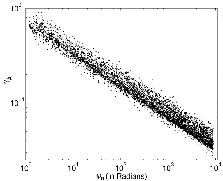
Figure 3: Efficiency factor $\gamma_{\rm A}$ obtained from numerical simulations. The plot shows 5000 binary pulsar systems with random parameters. The distributions are uniform in the ranges given by $N_{P_{\rm orb}}\in[2.0;20.0]$, $\varphi_{n}\in[1.2;9000]$, $\eta\in[-0.5;0.5]$ and $\phi_{orb}\in[-\pi;\pi]$.

3.3 Summary

We have now completed our Fourier analysis of a periodic signal whose phase is modulated by circular orbital motion. For an observation of finite duration, we can summarize our results as follows :

• The basic analytical solution is given by Eq. (12).

• The power spectrum is $N_{P_{\rm orb}}$-periodic over a finite frequency range about each harmonic.

• The phase in Fourier space is unpredictable a priori because $N_{P_{\rm orb}}$ and $\phi_{\rm orb}$ are unknown.

• A numerical simulation including an FFT is more efficient than a direct computation of Eq. (12).

• The statistical properties of white noise do not favor any particular periodicity. The particular signature of a pulsar signal whose phase is modulated by a circular orbital motion consequently provides an opportunity for an incoherent detection of weak pulsar signals in broadband noise.

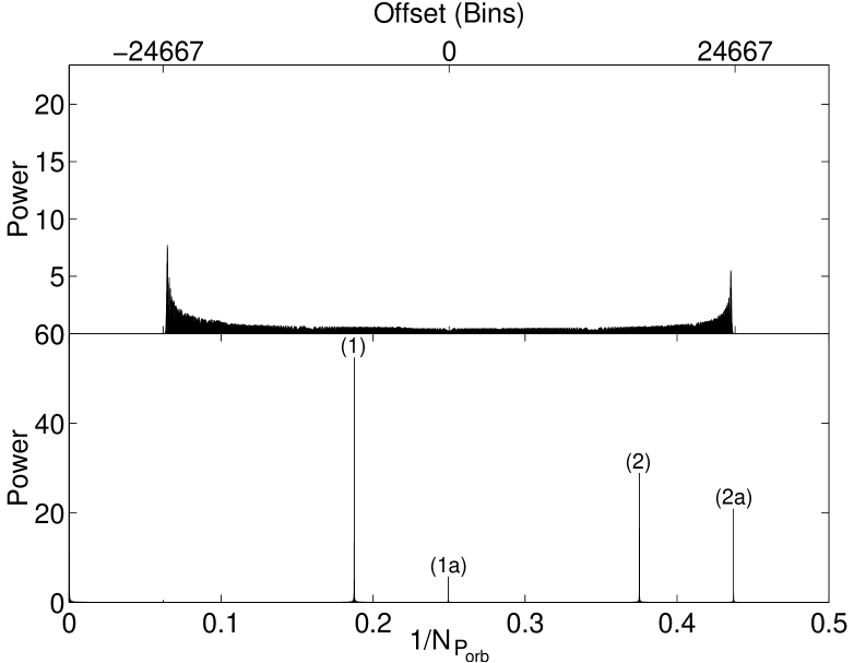
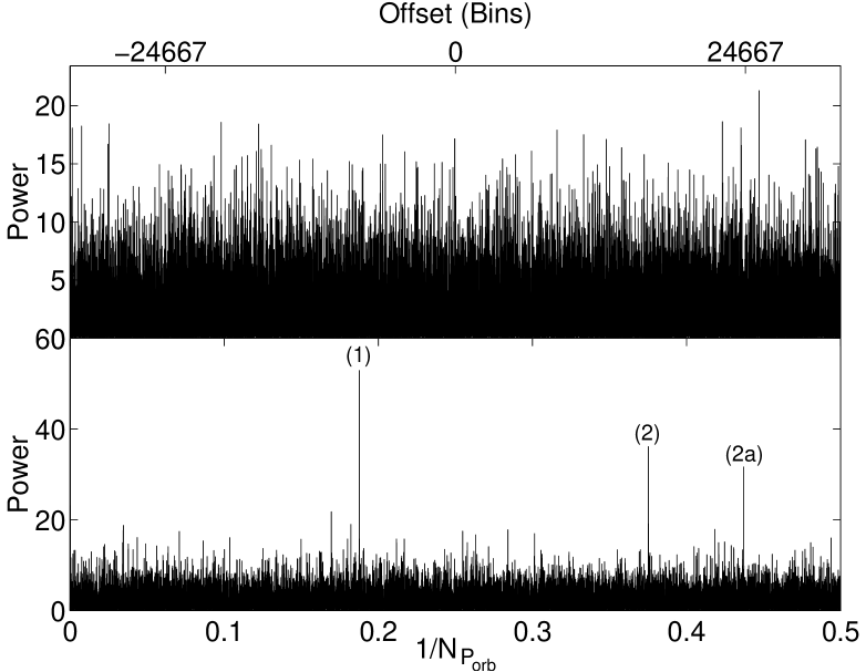
Figure 4: The binary system is described by $\nu_{\rm psr}=1$ KHz, $P_{\rm orb}=1.5$ hours, M₂ = 0.8 M_⊙ and $\phi_{orb}=53^{o}$ so that $\varphi_{1}=4571$ radians, $N_{P_{\rm orb}}=5.34$ and $\eta=0.23$. Upper plots show raw power spectra as obtained from a direct DFT of a noiseless/noisy observation (left/right respectively). Lower plots show ${\cal Q}$. The pulsar is detected at $1/N_{P_{\rm orb}}$ as shown by feature (1). The second harmonic is indicated by feature (2). Features (1a) and (2a) are essentially caused by beating of $N_{P_{\rm orb}}$ with bins in ${\cal P}$-space. The relative position of (1a)/(1) and (2a)/(2) is given by 1+Frac$[N_{P_{\rm orb}}]$. Multiplicative weighting windows could almost remove such features caused by spectral leakage effects (see Sec. 3.2.2).

We have considered pulsars in circular orbits. The case of eccentric orbits is extremely difficult to solve analytically. The envelope of the Fourier response becomes very complicated and can not be described by simple Bessel functions. However, the sideband spacing still remains the same and therefore produces a periodic sequence as in the case of circular orbits.

We have not considered non-uniform sampling as may happen for long observations due to Doppler correction for the observatory, either earthbound or satellite-borne. We assumed that the time series has been resampled with equal intervals for an observation in the solar system barycentric frame.

In Sec. 4, we briefly present three pulsar search techniques widely used in radio/X-ray astronomy and investigate their limiting sensitivity to binary pulsars in close circular orbits. In Sec. 5, we use the results of the present section to develop a very efficient implementation of the Phase Modulation Searching method (Ransom 1999). Eventually, we compare the efficiency of these recovery techniques and discuss the detectability of a range of binary pulsars in ultra-short circular orbits.

4 Searching for pulsars in close binary systems

When a pulsar signal is present in a time series, which in the case of radio observations has already been corrected for the dispersion due to its passage through the interstellar medium, it manifests itself as a set of discrete harmonics in the Fourier spectrum. The number of significant harmonics depends on the duty cycle of the pulsar (fractional on-time of the pulsar signal). Whereas ordinary pulsars have a typical duty cycle of about 4% (indicating about 12 significant harmonics in the spectrum), the millisecond pulsars seem to have a duty cycle of about 10% (about 5 harmonics). In the population of X-ray pulsars, the High Mass X-ray Binary pulsars have complex pulse profiles and thus have a few significant harmonics. However, some Low Mass X-ray Binary pulsars, including the only known millisecond pulsar among them, show nearly sinusoidal pulsations. Naturally, whenever we have more than one harmonic, “harmonic-folding” (Bhattacharya 1998) will improve the probability of detection when compared to looking for statistically significant isolated harmonics in the power spectrum.

In the case of solitary pulsar signals, harmonics are essentially confined to one bin whose power is decreased by ${\rm sinc}^{2}({\rm Min}[|{\rm Frac}[n\eta]|,1-|{\rm Frac}[n\eta]|])$, where $n$ is the harmonic number ; it is important to account for the spectral leakage factor $\eta$ because we will compare different recovery techniques that are not equally affected by such an effect. In a way similar to that of Johnston & Kulkarni (1991), we define the efficiency factor $\gamma$, such that a binary pulsar must, on average, carry $\gamma^{-1}$ more pulsed flux density than its virtual solitary counterpart to be detected with the same significance level. We now present several methods and calculate their $\gamma$ either from theoretical predictions or numerical simulations. We will compare and discuss their performances in fuller details in Sec. 6.

• Method A

  Consider a signal emitted by a pulsar in a binary system with a circular orbit. This signal is corrected to the solar system barycenter if necessary and uniformly resampled. Then, we simply search for statistically significant peaks in the discrete power spectrum – henceforth referred to as ${\cal P}$-space. As seen in Sec. 3.2.1, a given harmonic number $n$ will be spread out over $I(\varphi_{n},N_{P_{\rm orb}})$ bins. The efficiency factor $\gamma_{\rm A}$ is plotted as a function of $\varphi_{n}$ for 5000 systems with random parameters in Fig. 3. The distributions are uniform in the ranges given by $N_{P_{\rm orb}}\in[2.0;20.0]$, $\varphi_{n}\in[1.2;9000]$, $\eta\in[-0.5;0.5]$ and $\phi_{orb}\in[-\pi;\pi]$. Clearly, $\gamma_{\rm A}$ is strongly correlated with $\varphi_{n}$. The dispersion about the least-square-fit line

  $$\gamma_{\rm A}\simeq[0.74\pm 0.1]\,\varphi_{n}^{-0.325}$$ (18)

  is mostly caused by spectral leakage effects. Therefore, $\gamma_{\rm A}$ is maximized when $N_{P_{\rm orb}}$ and $\eta$ are close to integer values.

  As $\varphi_{n}\propto a_{1}$ and $\gamma_{\rm A}$ varies little with orbital period, we can see in Fig. 3 that close binaries are easier to detect than wide binaries. This is because a pulsar with a relatively small $\varphi_{n}$ experiences less acceleration.

  In the worst case, sensitivity limits are decreased by a factor of about 30 when compared to a solitary pulsar.

• Method B

  Numerous authors have developed techniques to correct for the Doppler smearing caused by the orbital motion. However, a complete coherent recovery involves searching in a parameter space defined by a large range of keplerian parameters. This is computationally unfeasible for the present day technology. As a compromise, some authors (Middleditch & Priedhorsky 1986; Anderson et al. 1990; Wood et al. 1991; Camilo et al. 2000; Johnston & Kulkarni 1991) have attempted a constant acceleration correction. Our simulations showed, in good agreement with Camilo et al. (2000), that almost 100% of the pulse strength is on average recoverable for all orbital phases if $N_{P_{\rm orb}}\raisebox{-1.29167pt}{\mbox{$\stackrel{{\scriptstyle<}}{{{}_{\sim}}}\,$}}1/7$. The efficiency of constant acceleration searches can therefore be expressed as

  $$\gamma_{\rm B}\simeq\frac{1}{\sqrt{7\;N_{\rm P_{\rm orb}}}}\,.$$ (19)

  Clearly, constant acceleration searches perform well when the observing time is much less than the orbital period. The efficiency of such a method can be expressed in various ways. We have estimated $\gamma_{\rm B}$ in order to maximize the recovery for the smearing due to the time-dependent Doppler effect experienced by the binary pulsar. This method basically allows for searching the whole time series with negative and positive acceleration values, including zero acceleration. Therefore in practice, it includes Method A which may itself prove more sensitive when $N_{\rm P_{\rm orb}}$ is large. However, Method B and $\gamma_{\rm B}$ will henceforth refer to Eq. (19) as aiming for a “non zero” constant acceleration correction.

• Method C

  Another method widely used in X-ray astronomy consists of dividing a long time series into $N_{\rm s}$ sub-segments in order to reduce the frequency resolution so that the Doppler shifted pulsar signal remains essentially confined to one bin in ${\cal P}$-space (van der Klis 1989). The $N_{\rm s}$ short power spectra are then incoherently summed. The stacked power spectrum is subsequently searched for statistically significant peaks.

  Using confidence levels instead of signal-to-noise ratio (SNR) is of great importance here because the noise distribution itself is modified in this process. The efficiency factor $\gamma_{\rm C}$ can therefore be measured as follows : let us define $\chi_{\alpha}^{D_{f}}$ as the inverse cumulative density function for a chi-squared distribution with $D_{f}$ degrees of freedom at the confidence value $\alpha$ ($D_{f}=2\,N_{\rm s}$). By analogy with Sec. 3.2.4, we can define $X=\sum_{k=1}^{N_{\rm s}}|\tilde{x}_{k}|^{2}$ so that Prob$(X>\chi_{\alpha}^{D_{f}})=\alpha$. The average expectation of $X$ is given by $\chi_{1/2}^{D_{f}}$. When $D_{f}$ is large, the noise distribution approaches a gaussian and $\chi_{1/2}^{D_{f}}$ coincides with the average value of $X$. Also, when $D_{f}$ is large, the noise can be considered additive in power instead of in Fourier amplitude (Vaughan et al. 1994; Groth 1975). Hence, $\gamma_{\rm C}$ is given by

  $$\gamma_{\rm C}=\sqrt{\begin{array}[]{lcl}\chi_{\alpha}^{2}&-&\chi_{1/2}^{2}\\[4.26773pt] \hline\cr\\[-7.11317pt] \chi_{\alpha\,N_{\rm s}}^{2\,N_{\rm s}}&-&\chi_{1/2}^{2\,N_{\rm s}}\end{array}}\,.$$ (20)

  $\gamma_{\rm C}$ must be evaluated at discrete values given by $N_{\rm s}=2^{p},p\in{\mathbb{N}}$. In a sense, such an approach is very simple as $\gamma_{\rm C}$ depends only on $I(\varphi_{n},N_{P_{\rm orb}})$, but we can not immediately recover any orbital parameter. However, this method can be very powerful (see Sec. 6 for a fuller discussion).

5 Partial coherence
recovery technique

We now describe our Partial Coherence Recovery Technique. We start with an observation of radio/X-ray pulsations which has been Fourier Transformed as in Method A. Somewhere in ${\cal P}$-space lies a set of $N_{P_{\rm orb}}$-periodic sequences centered on harmonic frequencies of $N_{P_{\rm psr}}$. This periodicity, often buried beneath the noise, can be detected by computing a short DFT of ${\cal P}_{n}$ of length $K\sim I(\varphi_{n},N_{P_{\rm orb}})$ bins. Subsequently, we define ${\cal Q}=|\tilde{{\cal P}}_{n}|^{2}$, hereby defining ${\cal Q}$-space as some sort of ’incomplete’ T-space (T-space is obtained by an inverse DFT of Fourier amplitudes whereas we perform a forward DFT of Fourier powers). Searching for statistically significant peaks in ${\cal Q}$ would reveal the presence of a sufficiently strong pulsar signal at $1/N_{P_{\rm orb}}$ if $N_{P_{\rm orb}}>2$ (see Shannon’s Sampling Theorem - Shannon 1948). Thus, a detection is made as shown in Fig. 4. Both pulsar and orbital phases are lost in ${\cal Q}$-space, hence we call this technique Partial Coherence Recovery Technique (henceforth referred to as PCRT and Method D).

The following sections are devoted to pulsar signal detection and estimation, where detection is the task of determining if a pulsar signal is present in an observation, while estimation is the task of obtaining the values of the parameters describing the signal.

5.1 Detection

Since ${\cal P}_{n}$ is localized in ${\cal P}$-space and its extent unknown a priori, we must compute many DFTs at all possible harmonics of $N_{P}{{}_{\rm psr}}$ with various widths $K$. We subsequently use a set of sliding windows ${\cal W}$ and define ${\cal W}_{K,\ell}$ as the window of size $K$ centered on bin $\ell$. A sufficiently strong pulsar signal will be detected when ${\cal W}_{K,\ell}$ contains ${\cal P}_{n}$, i.e. $\ell\approx N_{P_{\rm psr}}$ and $K\raisebox{-1.29167pt}{\mbox{$\stackrel{{\scriptstyle>}}{{{}_{\sim}}}\,$}}I(\varphi_{n},N_{P_{\rm orb}})$.

Table 1: Fourier spectrum statistics. The kurtosis is measured on real and imaginary Fourier samples obtained from an exponentially distributed noise. A normal distribution has Kurtosis = 3. Higher values indicate leptokurtic distributions.

$K$	16	32	64	128	256	512	1024
Kurtosis	3.83	3.51	3.25	3.10	3.05	3.02	3.01

5.1.1 Sizes of the short DFTs

Since $P_{\zeta,n}$ is compact, $K$ must be $\sim I(\varphi_{n},N_{P_{\rm orb}})$ bins to achieve optimal detectability. Computing DFTs of random sizes is not achieved efficiently with modern algorithms, so we must compromise our sensitivity to minimize the computational effort by computing the DFTs using FFTs of dyadic length $K=2^{p},p\in{\mathbb{N}}$.

We need a well-behaved noise probability density function to compute appropriate detection levels. The noise distribution in ${\cal Q}$-space will approach gaussian statistics when $K$ is large enough (Central Limit Theorem). In Table 1, we show that such a distribution is leptokurtic for small values of $K$. This implies that more probability is distributed in the tail, so a larger number of high noise values must be expected. In other words, a search code would pick up more noise samples than we would expect on the basis of a gaussian distribution. The lower limit to assign to $K$ is however somewhat arbitrary as one has to define a criterion of exclusion where an estimator deviates from gaussian statistics; we chose $K_{\rm min}=2^{8}$.

The upper limit is determined by ${\rm Max}[I(\varphi_{n},N_{P_{\rm orb}})]$. It corresponds to “the” extreme astrophysical case where the number of bins over which the signal power is distributed is maximum. Let us consider a hypothetical 0.5 ms pulsar of 1.4 M_⊙ with a companion star of 1.4 M_⊙ in a binary system with a circular orbit of 3.728 hours; $i=90$ degrees, $N_{P_{\rm orb}}$ = 2 and $n$ = 2. We use the second harmonic as we consider an extreme case and therefore aim to maximize $\varphi_{n}$. The orbital velocity of the pulsar $v_{\rm max}=279$ km/s and the second harmonic power spreads over about $200\times 10^{3}$ ($\raisebox{-1.29167pt}{\mbox{$\stackrel{{\scriptstyle<}}{{{}_{\sim}}}\,$}}2^{18}$) bins. We therefore take an upper limit $K_{\rm max}$ of $2^{18}$.

The number of values possibly taken by $K$ is given by $N_{K}=1+\log_{2}K_{\rm max}-\log_{2}K_{\rm min}$. In the case we considered above, $N_{K}=11$.

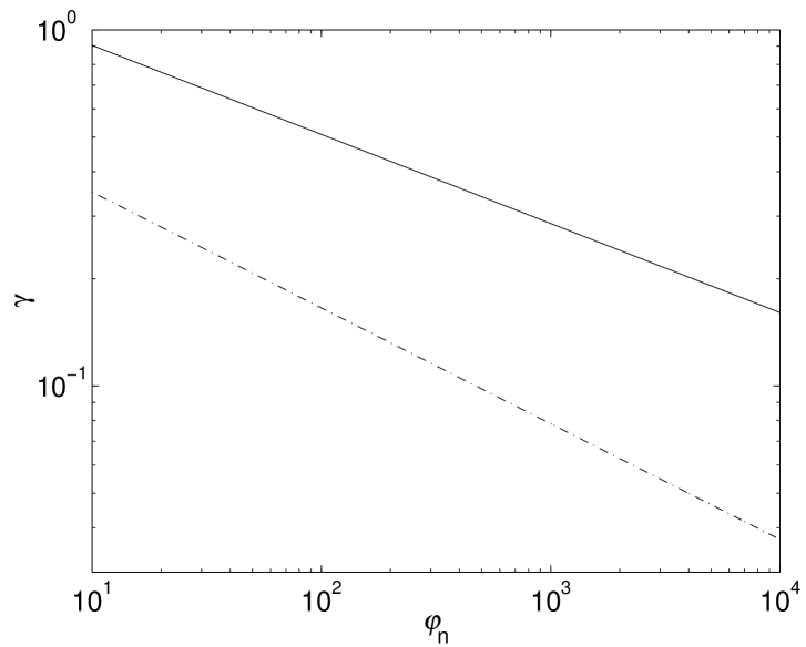
Figure 5: The dot-dashed curve (Method A) is given by Eq. (18). The solid curve represents Method D (PCRT).

5.1.2 Sliding windows

The ideal situation occurs when the power spectrum of ${\cal W}_{K,\ell}$ can be computed at all possible frequency bins $\ell$ where a pulsar signal is possibly expected. Let us denote that number by $L$. If the sampling time is 0.1 ms and minimum pulsar period 0.5 ms, $L\approx N/5$. The number of operations required to compute all FFTs is given by (see Appendix C.1)

$${\cal O}_{\rm FFT}\simeq 2^{N_{K}}LK_{\rm min}\left[\,\log_{2}K_{\rm min}+N_{K}-2\,\right]\,.$$ (21)

In our example where $N_{K}=11$ and $K_{\rm min}=256$, ${\cal O}_{\rm FFT}\approx 9\,L\times 10^{6}$. If $N=2^{28}$, ${\cal O}_{\rm FFT}\approx 4.8\times 10^{14}$ which requires about 5.6 days of computations on a 1 GigaFLOPS machine. This is prohibitive. An alternative is to decrease the fraction of overlap $\varrho$ between consecutive ${\cal W}_{K,\ell}$ where $\varrho=1-\rho/K$, $\rho\in[1:K_{\rm min}-1]$ (note that $\varrho$ is a fraction, whereas $\rho$ denotes a number of bins). The number of operations then reduces to (see Appendix C.2)

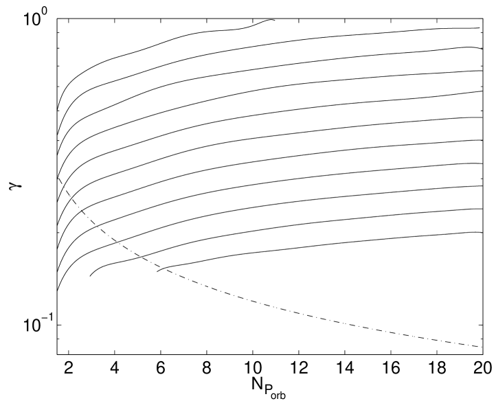
Figure 6: The dot-dashed curve (Method B) is given by Eq. (19). Note that $\gamma_{\rm B}$ scales with $N_{P_{\rm orb}}$. Solid curves (Method D) correspond to $K=2^{8}\ldots 2^{18}$ (upper curve is $K=2^{8}$). Higher $\gamma$ implies better sensitivity. Method D is superior to method B in nearly all cases.

$${\cal O}_{\rm FFT}\simeq\frac{L}{1-\varrho}\left[N_{K}\log_{2}K_{\rm min}+\frac{N_{K}(N_{K}-1)}{2}\right]\,.$$ (22)

If $\varrho=0.87$, ${\cal O}_{FFT}\approx 5.9\times 10^{10}$ which requires about 1 minute of computations on a 1 GigaFLOPS machine.

A sliding window of length $K$ must catch $P_{\zeta,n}$ with $I(\varphi_{n},N_{P_{\rm orb}})\leq\varrho\,K$. For such signals where the probability of being entirely swept up by ${\cal W}_{K,\ell}$ is 1, at least 1-$\varrho$ fraction of the sliding window will convey only noise. In that sense and because ${\cal W}_{K,\ell}$ is evaluated for a small number of sizes $N_{K}$, we can say that our algorithm suffers from our limited computation power.

The number of correlated spectral samples eventually obtained after processing $L$ bins with a single sliding window of length $K$ amounts to $L/2(1-\varrho)$. Overlapping windows cause another intrinsic problem, namely the correlation of random components. If ${\cal W}_{K,\ell}$ is defined with a Boxcar function, successive $\tilde{{\cal W}}_{K,\ell}$ will be $100\leavevmode\nobreak\ \times\leavevmode\nobreak\ \varrho$ % correlated. This implies that the number of uncorrelated spectral samples obtained after processing $L$ bins with a single window of size $K$ drops back to $L/2$.

5.1.3 Detection levels

${\cal W}_{K,\ell}$ contains a chi-squared distributed broadband noise, and may also include a $N_{P_{\rm orb}}$-periodic sequence caused by a signal. As seen in Sec. 3.2, such a sequence is very spiky. This comb of sidebands essentially decomposes into $H={\rm Int}[N_{P_{\rm orb}}/2]$ harmonics in ${\cal Q}$-space if $N_{P_{\rm orb}}>2$ (Shannon 1948). The presence of a sufficiently strong binary pulsar signal would be detected in ${\cal Q}$ at harmonics of its orbital period as shown in Fig. 4.

Table 2: Harmonic folding ambiguity. $L/N_{H}$ is given by Eq. (23) and $N=2^{28}$. $N_{A}$ denotes a number of combinations.

$H$	1	2	3	4	5	6	7	8	9
$L/N_{H}$	4	12	24	40	60	84	112	144	180
$N_{A}$	1	3	5	9	13	17	23	31	37

When $N_{P_{\rm orb}}>4$, it becomes useful to fold successive harmonics in ${\cal Q}$ to improve detection limits. Harmonic folding (Bhattacharya 1998) denotes the process of incoherently gathering harmonically related signal peaks in a power spectrum. For instance in Fig. 4, we clearly see that adding the two harmonics, namely features (1) and (2), will greatly improve the significance level of the detection.

Folding means incoherent addition of $H$ independent chi-squared distributed samples resulting in chi-squared distributed noise with $2H$ degrees of freedom. Since a detection has a statistical significance for a particular noise distribution, the number of uncorrelated spectral samples $N_{H}$ to be searched for a pulsar signal must be dealt with separately as a function of $H$ . In other words, the significance of a power obtained after folding 2 or 3 harmonics is different because the noise distribution itself depends on the harmonic fold number. Therefore, we define $N_{H}$ as the number of samples that can be folded a maximum of $H$ times in ${\cal Q}$-space ($H=1$ means no folding since we consider only harmonic number 1). A simple dichotomy gives

$$N_{H}=\frac{L}{2}\left[\frac{1}{H}-\frac{1}{H+1}\right]=\frac{L}{2\,H\,(H+1)}$$ (23)

where, for a given sliding window of size $K$, $L/2$ represents the total number of uncorrelated powers in ${\cal Q}$-space and the term within square brackets denotes the fractionnal amount of samples that can be folded a maximum of $H$ times.

Another complication arises because each frequency channel has a finite bandwidth. We can incoherently add bin number 10 with bin number 20, but also with bin number 19 or 21 depending whether $\eta<-0.25$, $|\eta|<0.25$ or $\eta>0.25$. This ambiguity becomes extremely complicated when $H$ increases and requires a large amount of book-keeping. We define $N_{A}$ as a measure of such an ambiguity. In other words, $N_{A}$ represents the number of possible combinations in folding $H$ harmonics. As shown in Table 2, $N_{A}$ increases with harmonic number $H$. A comprehensive search must cover all possibilities. Therefore, the significance level of a detection obtained after folding must take into account the number of combinations $N_{A}$ as well as the appropriate noise distribution.

The detection level at harmonic number $H$ is consequently given by $\chi_{\alpha/N_{A}N_{H}H_{\rm max}}^{2H}$, where $H_{\rm max}=9$ in our case. We used a confidence level $\alpha$ of 1% to estimate $\gamma_{\rm D}$.

5.2 Estimation

Once a significant peak is detected and localized both in ${\cal P}$-space and ${\cal Q}$-space, we can perform efficient complex cross-correlations of length $\sim I(\varphi_{n},N_{P_{\rm orb}})$ with a relatively small number of functions $\tilde{\zeta}_{n}$ given by Eq. (14). Such a coherent recovery of a suspected pulsar signal is very computationally efficient and extremely sensitive. As we showed in Sec. 3.2.3, $\zeta_{n}$ is defined by four parameters :

1. $P_{\rm orb}$ is obtained directly from ${\cal Q}$ where a pulsar signal has first been suspected as in Fig. 4. The accuracy to which this parameter is known improves with $\varphi_{n}$ and $T_{\rm obs}$.

2. $\varphi_{n}$ can be approximately estimated given $N_{P_{\rm orb}}$ and the length $K$ of the current sliding window. However, a more accurate estimation can be obtained efficiently by performing sliding FFTs of various lengths about $K$ in order to maximize the SNR at the frequency corresponding to $1/N_{P_{\rm orb}}$. Since we assumed circular orbits $P_{\xi,n}$ is symmetric, so this process also yields an approximate value of $\nu_{\rm psr}$.

3. $\phi_{\rm orb}$ can be obtained by performing complex cross-correlations in T-space. Since we work on a small number of Fourier amplitudes (as $I(\varphi_{n},N_{P_{\rm orb}})\sim 2\,N_{P_{\rm orb}}\,\varphi_{n}$ bins), we can inverse Fourier Transform ${\cal Q}$ and complex cross-correlate with our reference function $\zeta_{n}$ given by Eq. (14) and $\phi_{\rm orb}=0$. The initial orbital phase $\phi_{\rm orb}$ can be easily recovered if $N_{P_{\rm orb}}$ is known. In practice $\nu_{\rm psr}$ is approximated when computing $\zeta_{n}$.

4. $\eta$ gives $\nu_{\rm psr}$ within about half a frequency bin of precision. This parameter can be obtained by complex cross-correlating ${\cal Q}$ with $\tilde{\zeta}_{n}$ using previous estimates of $N_{P_{\rm orb}}$, $\varphi_{n}$ and $\phi_{\rm orb}$.

The pulsar frequency and all measurable binary parameters are therefore known at the end of this procedure. Such a recipe holds for pulsars in circular orbits. If the periodic sequence in ${\cal P}$-space is caused by a pulsar in eccentric orbit, another procedure must be used and further processing is required. We have not investigated such a case as our aim is to give a complete recipe for searching for pulsars with circular orbital motion. The case of eccentric orbits should however receive full attention in the context of the Phase Modulation Searching method.

6 Discussion

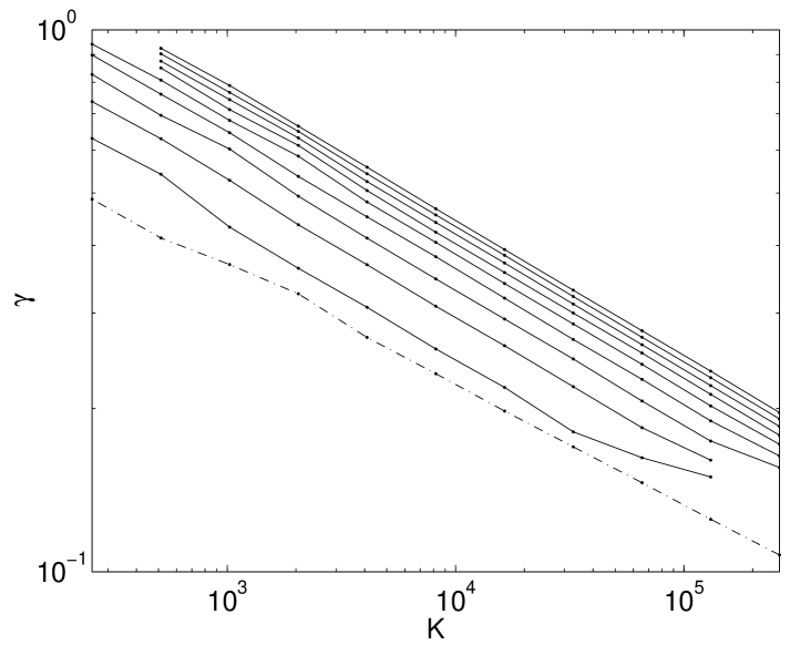
Figure 7: The dot-dashed curve (Method C) is given by Eq. (20). $\gamma_{\rm C}$ depends only on $K\sim 2\,N_{P_{\rm orb}}\,\varphi_{n}$. Solid curves (Method D) correspond to $N_{P_{\rm orb}}\in[2\,H;2\,(H+1)[$ where $H=1\ldots 9$ is the harmonic fold number defined in Sec. 5.1.3. The upper curve corresponds to $H=9$. The $\gamma$ values are estimated at $K=2^{p}$, $p\in{\mathbb{N}}$.

We have considered binary pulsars in circular orbits in Sec. 2. In Sec. 3, we derived the analytical solution to the problem of Fourier analysis of such pulsar signals in the solar system barycentric frame, in the continuous and discrete regimes. We found that each harmonic in the power spectrum of such signals spreads over about $2\,\,N_{P_{\rm orb}}\,\varphi_{n}$ bins, within which it is $N_{P_{\rm orb}}$ periodic. We suggested two ways of modelling the Fourier response of such pulsar signals and estimated the computational cost of these methods. In Sec. 4, we have estimated the detectability of such pulsars (assuming that all parameters were unknown) using three widely used methods (Method A : standard Fourier analysis - Method B : constant acceleration correction - Method C : stack searches) for which we derived efficiency factors $\gamma$. In Sec. 5, we presented a detailed description of our Partial Coherence Recovery Technique (Method D) which takes advantage of the periodicity in the power spectrum of a binary pulsar signal (see Sec. 3) to implement a pulsar search algorithm based on the Phase Modulation Search method (Ransom 1999). In this section, we present and discuss the sensitivity of all four techniques to close binary pulsars of different types with various companion masses and orbital periods.

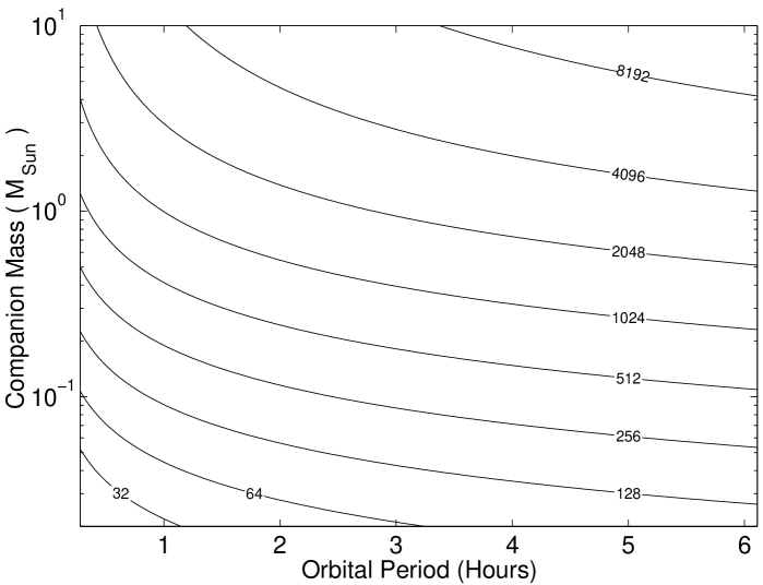
Figure 8: Contour map of $\varphi_{1}$ as a function of orbital period $P_{\rm orb}$ and companion mass M₂. We assumed $i=90^{o}$ and $\nu_{\rm psr}=250$ Hz. We recall that $\varphi_{1}\propto\nu_{\rm psr}\,\sin(i)$.

We have simulated $2^{17}$ random binary systems with

$$\indent\left\{\begin{array}[]{ll}\varphi_{1}&\in[1;10000]\\ N_{P_{\rm orb}}&\in[1.5;20]\\ \phi_{orb}&\in[-\pi;\pi]\\ \eta&\in[-0.5;0.5]\end{array}\right.$$

and calculated $\gamma_{\rm D}$ for each system individually. We compare our results with Method A, B and C on Fig. 5, 6 and 7. We recall that the sensitivity of pulsar search algorithms usually expressed in units of milli-Jansky is inversely proportional to $\gamma$.

As shown in Fig. 5, $\gamma_{\rm D}/\gamma_{\rm A}\raisebox{-1.29167pt}{\mbox{$\stackrel{{\scriptstyle>}}{{{}_{\sim}}}\,$}}3$ for all $\varphi_{n}$ and both methods are strongly correlated with $\varphi_{n}$. However, $\gamma_{\rm D}$ varies relatively little with $N_{P_{\rm orb}}$ as we can see in Fig. 6. Fig. 6 and 7 compare state-of-the-art methods in recovering smeared pulsar signals. Method D is significantly better than Method B when searching for very close binary systems with ultra-short orbital periods for which $N_{P_{\rm orb}}$ is large (e.g. $N_{P_{\rm orb}}=36$ for $P_{\rm orb}=10$ minutes and $T_{\rm obs}=6$ hours) and relatively small $\varphi_{n}$. Furthermore, $\gamma_{\rm B}$ in Fig. 6 represents an ideal case where it is possible to run a constant acceleration code on about one seventh of $P_{\rm orb}$, which is rarely the case as the orbital period is usually unknown. Therefore, we expect $\gamma_{\rm D}/\gamma_{\rm B}$ to be even larger. Another important consideration concerns the processing time. In Method B many long FFTs are taken repeatedly for each positive and negative acceleration trial for various data lengths, whereas in Method D only one long FFT is performed. The gain in processing time is considerable, especially when the range of orbital accelerations is large. Method D (PCRT) does not perform well when $N_{P_{\rm orb}}<2$ because a detection then relies on an aliased frequency component (Shannon 1948).

Fig. 7 demonstrates that Method D is always more sensitive than Method C. The reason is as follows : as seen in Sec. 3, a harmonic manifests itself in ${\cal P}$-space as a comb of sidebands separated by $N_{P_{\rm orb}}-1$ bins. These bins carry mostly noise and are co-added de facto in Method C. Whereas in Method D, we perform a spectral analysis which basically ignores them. However, Method C must be regarded as a useful method when compared to other standard searching techniques. Its good performance resides in the distribution of the noise itself, which becomes gaussian because many values are co-added, while, due to the decrease in frequency resolution, one deals with many fewer points hence improving the significance level of a detection. Such a method is also computationally very efficient. A clear drawback however resides in its lack of information about the binary system and poor frequency resolution.

In order to estimate the detectability of pulsars in ultra-short binary systems, we have plotted $\varphi_{1}$ as a function of $P_{\rm orb}$ and companion mass M₂ for a 4 ms pulsar in Fig. 8. This plot can be used for determining $\varphi_{1}$ for any particular pulsar. For example, let us consider a 8 ms pulsar in a binary system with $P_{\rm orb}=1$ hour and M${}_{2}=0.1$ M_⊙. The value of $\varphi_{1}$ is $128*4/8=64$ radians, where $4$ corresponds to the reference pulsar period in Fig. 8 and $8$ corresponds to the pulsar period we consider in milliseconds. Of course, $\varphi_{1}$ is a maximum value since we assumed an inclination angle of $90$ degrees but we recall that $\varphi_{n}$ scales directly with $\sin(i)$. Let us assume that $T_{\rm obs}=6$ hours, hence $N_{P_{\rm orb}}=6$. Looking up the $\gamma$ values for Method A, B, C and D in Fig. 5, 6 and 7, we see that this particular binary system would be best detected using Method D (PCRT) as $\gamma_{\rm D}>\gamma_{\rm C}>\gamma_{\rm A}>\gamma_{\rm B}$ (see Sec. 4 for an accurate definition of $\gamma_{\rm A}$ and $\gamma_{\rm B}$).

Of particular interest is the detection of pulsars with large companion masses such as Neutron Star - Neutron Star and Neutron Star - Black Hole systems in circular orbits. In such systems, millisecond pulsar signals are smeared over many bins in the Fourier spectrum because $\varphi_{n}$ is large. These systems are characterized by large accelerations which are usually not searched for in constant acceleration searches due to the large increase in the number of acceleration trials, which tremendously increases the processing time. Stack searches could be very useful in such a context. However, the PCRT is, on average, the most efficient and sensitive method available for detecting such extreme systems, with the proviso that the orbital period is short so that $N_{P_{\rm orb}}$ is greater than 2.

By direct and detailed comparison with other methods for correcting for the period variation caused by orbital acceleration, we find the PCRT is a very efficient method for detecting fast rotating radio/X-ray pulsars in binary systems, especially when $N_{P_{\rm orb}}$ is large. However, it requires long observations, and therefore is not well suited for direct application to all-sky pulsar surveys where integration times are usually less than half an hour. On the other hand, the method is ideally suited to long observations of globular and open clusters, steep spectrum point sources and X-ray point sources.

Appendix A

Main symbols defined in the text, with description and section of first use.

Symbol	Description	Section
$\chi^{D_{f}}$	Inverse cumulative density function for a chi-squared
	distribution with $D_{f}$ degrees of freedom.	4
$\gamma$	Efficiency of a binary pulsar search method ($\,0.0<\gamma<1.0\,$).	4
$H$	Harmonic fold number in ${\cal Q}$-space.	5.1.3
$I(\varphi_{n},N_{P_{\rm orb}})$	Width of $\tilde{\zeta}_{n}$ in bins (about $2\,\,N_{P_{\rm orb}}\,\varphi_{n}$ bins).	3.2.1
$K$	Length of a sliding window (${\cal W}_{K}$) in bins.	3.2.3, 5.1
$L$	Number of spectral samples searched for a pulsar signal in ${\cal P}$-space.	5.1.2
$\eta$	Spectral leakage factor : $\eta\in[-0.5;0.5]$ .	3.2.3
$N$	Number of equally spaced sampling points in T-space.	3.2.1
$N_{A}$	Number of possible harmonic fold combinations.	5.1.3
$N_{H}$	Number of samples which can be folded exactly $H$ times.	5.1.3
$N_{K}$	Number of sliding windows ${\cal W}_{K}$ used in the analysis.	5.1.1
$N_{\rm s}$	Number of sub-segments used in Method C.	4
$P_{\zeta,n}$	Power spectrum of $\tilde{\zeta}_{n}$ ($\sim I(\varphi_{n},N_{P_{\rm orb}})$ bins wide).	3.2.1
${\cal P}_{n}$	Noisy $P_{\zeta,n}$.	3.2.4
${\cal Q}$	Power spectrum of ${\cal P}_{n}$.	5
$\varrho$	Percentage of overlap between consecutive ${\cal W}_{K}$.	5.1.2
$\rho$	Number of overlapping bins between consecutive ${\cal W}_{K}$.	5.1.2
$\tilde{\zeta}_{n}$	Discrete Fourier response of the $n^{\rm th}$ harmonic of a noiseless binary pulsar signal
	of constant amplitude, shifted back to the origin of the frequency scale.	3.2.1
$W$	Observing window e.g. Boxcar ($W_{\rm B}$).	3.1
${\cal W_{K}}$	Sliding window of length $K$.	5.1
$\varphi_{n}$	Half the phase rotation experienced by the $n^{\rm th}$ harmonic of the pulsar signal
	during the orbit, in radians : $\varphi_{n}=2\pi n\nu_{\rm psr}\left[a_{1}\sin(i)/{\rm c}\right]$.	2
$\phi_{\rm orb}$	Initial orbital phase in radians, measured from superior conjunction of the pulsar.	2
$\nu_{\rm psr}$ , $N_{P_{psr}}$	Observed pulsar rotation frequency in Hz and Fourier bins, respectively.	2, 3.2.1
$\nu_{\rm orb}$ , $N_{P_{\rm orb}}$	Observed pulsar orbital frequency in Hz and Fourier bins, respectively.	2, 3.2.1

Appendix B

We derive the mathematical proof of Eq. (7). We shall demonstrate that

$$e^{\,jz\cos\theta}=\sum_{k=-\infty}^{\infty}j^{k}\,J_{k}(z)\,e^{\,jk\ theta}\,.$$ (24)

By definition,

$$e^{\,jz\cos\theta}=\cos(z\cos\theta)+j\sin(z\cos\theta)$$ (25)

where, according to Eqs. (9.1.44) and (9.1.45) in Abramowitz & Stegun 1974,

$$\cos(z\cos\theta)=J_{0}(z)+2\,\sum_{p=1}^{\infty}(-1)^{p}\,J_{2p}(z)\,\ cos(2p\,\theta)$$ (26)

$$\sin(z\cos\theta)=2\,\sum_{p=0}^{\infty}(-1)^{p}\,J_{2p+1}(z)\,\cos(\,[2p+1]\,\theta)\,.$$ (27)

Since $j=(-1)^{1/2}$, Eq. (27) can be rewritten as

$$\sin(z\cos\theta)=\frac{2}{j}\,\sum_{q=1/2}^{\infty}(-1)^{q}\,J_{2q}(z)\ ,\cos(2q\,\theta)$$ (28)

where $q=p+\frac{1}{2}$. Combining Eqs. (26) and (28) in (25) yields

$$e^{\,jz\cos\theta}=J_{0}(z)+2\,\sum_{k=1}^{\infty}(-1)^{k/2}\,J_{k}(z)\,\cos(k\,\theta)\,.$$ (29)

Since $\cos(k\,\theta)=\left[e^{\,jk\,\theta}+e^{-jk\,\theta}\right]/2$, we get

$$e^{\,jz\cos\theta}=J_{0}(z)+\sum_{k=1}^{\infty}\left[\,j^{k}\,J_{k}(z)\,e^{\,jk\,\theta}+j^{k}\,J_{k}(z)\,e^{\,-jk\,\theta}\,\right]\,.$$ (30)

According to Eq. (9.1.5) in Abramowitz & Stegun 1974 : $J_{k}(z)=j^{-2k}\,J_{-k}(z)$. Therefore,

$$e^{\,jz\cos\theta}=J_{0}(z)+\sum_{k=1}^{\infty}\left[\,j^{k}\,J_{k}(z)\,e^{\,jk\,\theta}+j^{-k}\,J_{-k}(z)\,e^{\,-jk\,\theta}\,\right]$$ (31)

which simplifies to

$$e^{\,jz\cos\theta}=\sum_{k=-\infty}^{\infty}j^{k}\,J_{k}(z)\,e^{\,jk\,\ theta}\,.$$ (32)

We note that in Eq. (7), $j^{k}$ has been replaced by its equivalent exponential notation $e^{\,jk\pi/2}$.

Appendix C

C.1 Determination of Eq. (21)

Let us consider a given frequency channel and compute $N_{K}$ FFTs of length $K\in[K_{\rm min}\ldots K_{\rm max}]$. The number of operations required for an FFT of length $K$ is given by $K\log_{2}K$. Therefore,

$${\cal O}_{\rm FFT}=K_{\rm min}\log_{2}K_{\rm min}+\ldots+[\,2^{N_{K}-1}K_{\rm min}\,]\,\log_{2}\,[\,2^{N_{K}-1}K_{\rm min}\,]$$ (33)

which can be rewritten as

$${\cal O}_{\rm FFT}=K_{\rm min}\left[\,\log_{2}(K_{\rm min})\sum_{k=0}^{N_{K}-1}2^{k}+\sum_{k=0}^{N_{K}-1}2^{k}k\,\right]\,.$$ (34)

The summations can be explicitly computed so that

$${\cal O}_{\rm FFT}=K_{\rm min}\left[\,\log_{2}(K_{\rm min})\,[\,2^{N_{K}}-1\,]+[\,2^{N_{K}}(N_{K}-2)+2\,]\,\right]\,.$$ (35)

Assuming $2^{N_{K}}\gg 1$, Eq. (35) subsequently reduces to

$${\cal O}_{\rm FFT}\simeq 2^{N_{K}}K_{\rm min}\left[\,\log_{2}(K_{\rm min})+N_{K}-2\,\right]\,.$$ (36)

Naturally, ${\cal O}_{\rm FFT}$ must be multiplied by $L$ hence Eq. (21).

C.2 Determination of Eq. (22)

We now consider $\rho>1$. The number of frequency channels at which a FFT of length $K$ is evaluated reduces to $L/K(1-\varrho)$. Therefore,

$${\cal O}_{\rm FFT}=\frac{L\,\left[\,K_{\rm min}\log_{2}K_{\rm min}\,\right]}{K_{\rm min}(1-\varrho)}+\ldots+\frac{L\,\left[\,2^{N_{K}-1}K_{\rm min}\log_{2}(2^{N_{K}-1}K_{\rm min})\,\right]}{2^{N_{K}-1}K_{\rm min}(1-\varrho)}\,.$$ (37)

This equation can be rewritten in a simple form as

$${\cal O}_{\rm FFT}=\frac{L}{1-\varrho}\,\left[\,N_{K}\log_{2}K_{\rm min}+\sum_{k=0}^{N_{K}-1}k\,\right]\,.$$ (38)

Subsequently, we obtain Eq. (22)

$${\cal O}_{\rm FFT}=\frac{L}{1-\varrho}\,\left[\,N_{K}\log_{2}K_{\rm min}+\frac{N_{K}(N_{K}-1)}{2}\,\right]\,.$$ (39)

References

- (1) Alpar M. A., Cheng A. F., Ruderman M. A., Shaham J. 1982, Nature, 300, 728
- (2) Radhakrishnan V. & Srinivasan G. 1982, Curr. Sci. 51, 1096
- (3) Backer D. C. et al. 1982, Nature, 300, 615
- (4) Pulsar Astronomy - 2000 and Beyond, IAU Colloquium 177, eds. M. Kramer, N. Wex, and N. Wielebinski (Astronomical Society of the Pacific, San Francisco, 2000), conference Proceeding
- (5) Middleditch J. & Priedhorsky W. C. 1986, ApJ, 306, 230
- (6) Anderson S. B. et al. 1990, Nature, 346, 42
- (7) Wood K. et al. 1991, ApJ, 379, 295
- (8) Ransom S. 2000 in Pulsar Astronomy - 2000 and Beyond, IAU Colloquium 177, eds. M. Kramer, N. Wex, and N. Wielebinski (Astronomical Society of the Pacific, San Francisco, 2000), conference Proceeding.
- (9) Camilo F. et al. 2000, ApJ., 535, 975
- (10) D’Amico N. et al. 2001, ApJ, in press (astro-ph/0010272)
- (11) Ransom S. et al. 2001, ApJ, in press (astro-ph/0010243)
- (12) Rasio F.A., Pfahl E. D., & Rappaport S. 2000, ApJ, 532, L47
- (13) Stella L., White N. E. & Priedhorsky W. 1987, ApJ, 312, L17
- (14) Lyne A. G. et al. 1990, IAU Circ. 4974
- (15) Bisnovatyi-Kogan G. 1989, Astrofizika, 31, 567
- (16) Ergma E. V. & Fedorova A. V. 1991, Pis ma Astronomicheskii Zhurnal, 17, 433
- (17) Fruchter A. S. & Goss W. M. 1990, ApJ, 365, L63
- (18) Fruchter A. S. & Goss W. m. 2000, ApJ, 536, 865
- (19) D’Amico N. et al. 1993, MNRAS, 260, L7
- (20) Biggs J. D. et al. 1994, MNRAS, 267, 125
- (21) Grenier I. A. 2001, A&A in prep.
- (22) Benacquista M., Portegies Zwart S., & Rasio F. 2001, Classical Quantum Gravity, in press (gr-qc/0010020)
- (23) Dhurandhar S. & Vecchio A. 2000, submitted to Phy. Rev. D (gr-qc/0011085)
- (24) Middleditch J., Mason K. O., Nelson J. E. & White N. E. 1981, ApJ, 244, 1001
- (25) Abramowitz M. & Stegun I., Handbook of Mathematical Functions with Formulas, Graphs, and Mathematical Tables (Dover Publications Inc., New York, 1974)
- (26) Harris F. J. 1978, Proc. I. E. E. E., 66, 51
- (27) Jenkins G. & Watts D., Spectral Analysis and its Applications (Holden-Day, Oakland, 1968)
- (28) Bhattacharya D. 1998, in The Many Faces of Neutron Stars,(NATO ASI Series), eds. J. van Paradis, A. Alpar, and L. Buccheri (Kluwer, Dordrecht, 1998), p. 103
- (29) Johnston H. M. & Kulkarni S. R. 1991, ApJ, 368, 504
- (30) van der Klis M., in Timing Neutron Stars,(NATO ASI Series), eds. H. Ögelman and E. P. J. van den Heuvel (Kluwer, Dordrecht, 1989), p. 27
- (31) Vaughan B. A. et al. 1994, ApJ, 435, 362
- (32) Groth E. 1975, ApJS, 29, 285
- (33) Shannon C. 1948, The Bell Sys. Tech. J., 27, 379