Measurement of radial velocities and velocity dispersion of stars in circumnuclear regions of galaxies using the 2D spectrosopy technique

Abstract

A procedure is described of construction of velocity fields and velocity dispersion of the stellar component in the central regions of galaxies on the basis of data obtained with the integral field spectrograph MPFS. Cross-correlation and Fourier quotients techniques adapted for 2D spectra reduction are used. A detailed discussion is given of the problems of providing for the instrumental profile in measuring the velocity dispersion. Using the existing version of the spectrograph, one can measure radial velocities and the dispersion of velocities to an accuracy of 5–10 km/s and 10–15 km/s, respectively. As an example the “double-barred” galaxy NGC 2950 is considered.

Key words:   galaxies: fundamental parameters — galaxies: individual: NGC 2950 — galaxies: spiral

1 Introduction

The present paper examines the problem of determination of two basic observational parameters that characterize the collective motion of stars in galaxies — radial velocity $v$ and velocity dispersion $\sigma$. The task has a half-a-century history, beginning with the pioneering observations by Minkowski (1954) to the latest papers concerning the relation between the mass of a central black hole and the velocity dispersion (Gebhardt et al., 2000). The procedure of measuring $v$ and $\sigma$ with the application of the technique of Fourier transform goes back to the classical works of Tonry and Davis (1979, hereafter TD) and Sargent et al. (1977, hereafter SSBS).

The methods of two-dimensional (2D) spectroscopy that have been advanced intensively over the last decade have made it possible to obtain two-dimensional mapping of velocities and velocity dispersions. In the case of disk galaxies this enables one to study non-circular motions in the region of the triaxial potential (bar) or near the active nucleus (see the survey of Arribas and Mediavilla, 2000). The multipupil spectrograph (MPFS) has been in operation at SAO RAS since 1990. It has been used to conduct similar observations (see, for instance, Afanasiev et al., 1996; Sil’chenko, 1998). In these papers, however, field velocities of stars and gas alone have been discussed. At the same time, the distribution of velocity dispersion gives information about the non-axisymmetrical shape of the gravitational potential. This is one of the key parameters in producing numerical dynamical models of galaxies (Khoperskov and Chulanova, 2001). The main methodological problem in measuring velocity dispersions is taking correct account of the variations of the instrumental profile of the spectrograph. A new version of the MPFS (in operation at BTA since 1998) constructs reliably the distributions of velocity dispersions in circumnuclear regions of galaxies, which is shown in the present paper.

The paper is organized as follows. The theory of methods of estimating $v$ and $\sigma$ is considered in Section 2. The problems of provision for the instrumental profile are discussed in Section 3, Section 4 gives a brief description of algorithms of analysis of MPFS spectra and errors that arise, the results of the galaxy NGC 2950 are presented in Section 5, conclusive remarks are collected in Section 6.

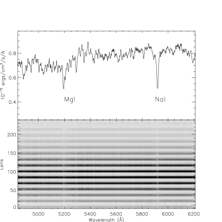
Figure 1: Example of MPFS spectra: the 2D spectrum of the galaxy NGC 2950 (bottom); the spectrum corresponding to the galaxy centre (top).

2 Methods of velocity and velocity dispersion measurement

2.1 General remarks

After a preliminary reduction, the MPFS observational data can be presented as two-dimensional spectra. The spectra from different spatial elements are brought to a common wavelength scale and arranged in the frame sequentially one above another. An example of such spectra is displayed in Fig.1. The spatial elements are constructed as small lenses and grouped into an array of $16\times 15$ pixels (micropupils). This corresponds to a field of view of $16^{\prime\prime}\times 15^{\prime\prime}$ on the sky.

Let us illustrate the idea of the methods of measuring $v$ and $\sigma$ by an individual spectrum of one spatial element. Let $G(\lambda)$ and $T(\lambda)$ are the observed spectra of the galaxy and a template star with the low-frequency component (continuum) subtracted. Typical examples of such spectra are shown in Fig. 2.

Figure 2: Spectra of the template star and of the S0 galaxy nucleus in the region of the doublet Na I obtained with the MPFS. The wavelength displacement of the galaxy spectrum is due to the Doppler shift, the line broadening is caused by the velocity dispersion along the line of sight.

The spectra are discretely sampled in wavelength $\lambda$.

The observed spectra need to be converted to a logarithmic scale in which the number of the spectral bin $n$ is related to the wavelength $\lambda$ by the expression

$$n=a\log(\lambda)+b,$$ (1)

where

$$\begin{array}[]{l}a=\log^{-1}(1+\Delta v/c),\\ b=-a\,\log(\lambda_{0}),\\ \end{array}$$ (2)

here $\Delta v$ is the step in velocity expressed in km/s, $c$ is the speed of light. The Doppler shift leads to uniform shift of the spectrum along the $n$ axis, irrespective of $\lambda$.

The galaxy spectrum may be approximately represented as a redshifted template spectrum convolved with a certain broadening function caused by inner motions of stars in the galaxy along the line of sight:

$$G(n)\approx\alpha T(n)\odot B(n-v),$$ (3)

the broadening function $B(n)$ in a first approximation can be represented by a Gaussian:

$$B(n)=\frac{1}{\sqrt{2\pi}\sigma}\exp\left(-\frac{n^{2}}{2\sigma^{2}}\right),$$ (4)

where $\alpha$ is the numerical coefficient, $v$ and $\sigma$ are the velocity and velocity dispersion along the line of sight.

The methods described below are based on calculations of a discrete Fourier transform defined for the function $F(n)$ as

$$\tilde{F}(k)=\sum_{n=0}^{N-1}F(n)\exp\left(-\frac{2\pi ink}{N}\right),$$ (5)

where $N$ is the number of points in the spectrum.

2.2 Cross-correlation method

The TD method is based on computation of a normalized cross-correlation function determined as

$$\begin{array}[]{l}C(n)=G(n)\otimes T(n)=\\ \qquad{\displaystyle\frac{1}{N\sigma_{g}\sigma_{t}}\sum_{m}G(m)T(m-n)},\\ \end{array}$$ (6)

where

$$\sigma_{g}^{2}=\frac{1}{N}\sum_{n}G(n)^{2},\,\sigma_{t}^{2}=\frac{1}{N}\sum_{n}T(n)^{2}.$$

After Fourier transformation, relationship (6) is written as

$$\tilde{C}(k)=\frac{1}{N\sigma_{g}\sigma_{t}}\tilde{G}(k)\tilde{T}^{*}(k).$$ (7)

where stars marks the complex conjugation.

Applying the procedure of cross-correlation to expression (3), one can readily obtain

$$C(n)=(T(n)\otimes T(n))\odot B(n-v),$$ (8)

i.e. the cross-correlation of the galaxy and star spectra is a convolution of the auto-correlation of the template star spectrum $T(n)$ (which provides information about the instrumental profile of the spectrograph) with the broadening function $B(n)$. The velocity $v$ is thus defined from the location of the cross-correlation function $C(n)$ maximum.

If the central peak of the cross-correlation function may be represented by a Gaussian with a dispersion $\mu$:

$$C(n)=c_{0}\exp\left(-\frac{(n-v)^{2}}{2\mu^{2}}\right),\\$$ (9)

and the peak of the auto-correlation function of the template spectra by a Gaussian with a dispersion $\sqrt{2}\,\tau$:

$$T(n)\otimes T(n)=t_{0}\exp\left(-\frac{n^{2}}{2(2\tau^{2})}\right),$$ (10)

then the square of the velocity dispersion is computed as

$$\sigma^{2}=\mu^{2}-2\tau^{2}.$$ (11)

In Fig. 3 are presented examples of the star and galaxy spectra prepared for cross-correlation, as well as the auto-correlation and cross-correlation peaks. In practice, due to the difference between the shape of the peak and the Gaussian one, to the contribution of the low-frequency component etc., the relation between $\sigma$ and $\mu$ may differ from (11), which introduces systematic errors into the estimate of $\sigma$.

A number of authors have proposed different modifications of the TD method for estimating the velocity dispersion. So, in the paper by Bottema (1988), straightforward use of relation (8) is made — the template auto-correlation function is convolved with Gaussians of different width until the cross-correlation peak shape is best reproduced.

Figure 3: Cross-correlation method. a, b are the spectra of a KİII star and the galaxy NGC 2950, the continuum subtracted; c, d are the spectra on a logarithmic scale with a step of $50\,km/s$, the boundaries of the spectra are multiplied by a sinusoid (see 4.1); e, f are the auto-correlation and the cross-correlation functions, the dotted line shows the approximation by a Gaussian.

We dwelled on the application of the empirical relation between the cross-correlation peak width and the velocity dispersion (see Nelson and Whittle, 1995). For this the template spectrum $T$ is convolved with Gaussians of different width $\sigma_{in}$, a cross-correlation function of broadened spectrum with $T$ is constructed, and using formula (11) the velocity dispersion $\sigma_{out}$ is formally determined. The relationship between $\sigma_{in}$ and $\sigma_{out}$, presented in Fig. 4, is approximated by a second-order polynomial:

$$\sigma_{in}=\sum_{i=0}^{2}\alpha_{i}\sigma_{out}^{i},$$ (12)

and is next used to estimate the dispersion from the cross-correlation peak width:

$$\sigma=\sum_{i=0}^{2}\alpha_{i}(\mu^{2}-2\tau^{2})^{i/2}.$$ (13)

2.3 The Fourier quotient method

This method was put forward in the SSBS paper. By applying Fourier transform (5) to (3) with provision for (4), obtain

$$\frac{\tilde{G}(k)}{\tilde{T}(k)}=\gamma\exp\left[-\frac{1}{2}\left(\frac{2\pi k\sigma}{N}\right)^{2}+\left(\frac{2\pi ikv}{N}\right)\right],$$ (14)

the real part in the exponent is defined by the velocity dispersion, the imaginary part — by the galaxy velocity. From relation (14) both the parameters ($\sigma$ and $v$) are formally determined, however, in practice, the ratio of the Fourier spectra of the object and template is more noisy than the cross-correlation function peak in the TD method. For this reason, it is simpler and more reliable to find $v$ from the shift of the cross-correlation peak; in this case the dispersion is estimated from:

$$\mbox{Re}\frac{\tilde{G}(k)\exp(-\frac{2\pi ikv}{N})}{\tilde{T}(k)}=\gamma\exp\left[-\frac{1}{2}\left(\frac{2\pi k\sigma}{N}\right)^{2}\right].$$ (15)

An example of approximation of the right side of (15) is shown in Fig. 5. It is necessary to choose the boundaries in frequency $k$, within which the fitting $k_{1}<k<k_{2}$ is made, in order to avoid the influence of high- and low-frequency noises. Our experience shows that $k_{1}=5-10$ and $k_{2}=50-120$ are optimum values for the number of points in the spectrum $N=500-1000$, being in good agreement with SSBS.

The advantage of the Fourier quotient method as compared to the cross-correlation one is that to estimate the dispersion in the SSBS-technique, no additional constraints on the shape of the cross-correlation and auto-correlation peaks are required, and only the assumption that broadening function (4) is of Gaussian shape is applied.

3 Instrumental profile problem

Expression (10) shows the fact that if the spectrograph instrumental profile is described by a Gaussian with a dispersion $\tau$, the width of the auto-correlation function of the spectrum produced is then $\sqrt{2}\,\tau$ (provided that the lines in the template spectrum can be considered to be infinitely narrow with respect to $\tau$). The width (and even the shape) of the instrumental profile of the spectrograph changes over the field (along the spectrograph slit and over the multipupil array), which is caused first of all by the spectrograph optics, precision of its adjustment and focusing. Besides, due to temperature fluctuations and flexures of the spectrograph, the quantity $\tau$ at each point is a function of time of observations and zenith distance.

Analysis of spectra taken with the new version of the MPFS shows that the spectrograph instrumental profile is time-stable, i.e. the variations of $\tau$ during the observing night can be neglected. In this case, the profile width is defined only by the coordinates of the spatial element a given spectrum corresponds to: $\tau=\tau(x,y)$.

Fig. 6 presents estimates of the MPFS profile width for different spectra (a He-Ne-Ar lamp comparison spectrum, field-of-view defocused template star spectrum, twilight sky spectrum). The measurements made from the comparison spectrum are systematically larger by 20–30 km/s (about 30% of the mean). This is connected with the fact that the entrance pupil image for the calibration beam is displaced with respect to the pupil position when observing the object. It can be seen from Fig. 6 that the profile width variations are $\pm(10\div 20)\%$ of the mean value ($\tau\approx 70$ km/s).

We performed experiments using different methods of taking account of the systematic variations of the instrumental profile with the aim of reliable mapping of the velocity dispersion distribution $\sigma$ and came to a conclusion that the following procedure is the most correct and simple at the same time. A bright ($5^{m}-6^{m}$) template star is defocused over the whole array of micropupils ($16^{\prime\prime}\times 15^{\prime\prime}$). During moderate exposures (90–200 s) at the MPFS it is possible to take template spectra with high signal-to-noise ratio over the whole field. When analysing the galaxy spectrum by the TD and SSBS at each point of $(x,y)$, an individual template spectrum $T(x,\,y)$ is taken. Such a procedure takes actually full account of the effect of the instrumental profile, provided, of course, that the spectrograph is carefully focused before the observation.

4 Sequence of work with MPFS data

4.1 Preparation of spectra

Using the language IDL, we have written a package of programmes CROSSLIB which implements the methods presented in Sections 2 and 3. The initial data are 2D spectra of a galaxy and a star (Fig. 1) after preliminary reduction (bias correction, flat-fielding, cosmic hits removal, individual spectrum extraction from the CCD images and its conversion to a common linear wavelength scale, night-sky line subtraction, correction, if needed, for the effect of differential atmospheric refraction).

Figure 4: Relationship (12): $\sigma_{in}$ is the width of the smoothing Gaussian, $\sigma_{out}$ is the dispersion estimated from the cross-correlation peak width (dots). The solid line is the approximation by a second-order polynomial, the dotted line corresponds to the relation $\sigma_{out}$ = $\sigma_{in}$.

Figure 5: Approximation of function (15) by a Gaussian in the Fourier quotient method. The boundaries of fitting ($k_{1}$ and $k_{2}$) are marked.

After the preliminary reduction the continuum is subtracted from the spectra. Underestimation of the continuum level leads to appearance of a low-frequency component in the Fourier spectrum and, as a consequence, to greater noises for small $k$ in the SSBS method, and of a wide base in the auto-correlation and cross-correlation peaks in the TD method.

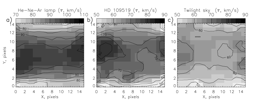
Figure 6: Instrumental profile of the MPFS (dispersion of the Gaussian $\tau$ in $km/s$) evaluated in the spectral range 5100–6100 Å, the spectrograph dispersion is $1.35$ Å/px: a — from the comparison spectrum, b — from the spectrum of the KIII star, c — from the twilight spectrum.

It is not infrequent that high-order polynomials are used to fit a continuum (Larsen et al., 1983). However, our experience of reduction has shown that the best result can be achieved if a spectrum smoothed by a median filter with a window of 150–200 pixels is taken as a continuum. In so doing, even the broadest absorption spectral features are practically undistorted.

The emission lines in the galaxy spectrum reduce the contrast of the cross-correlation peak. Depending on the number and the intensity of lines, different techniques can be employed to remove them. In most cases it suffices to approximate by a Gaussian the brightest line, determine the intensity of the rest of the lines with respect to it and subtract from the spectrum the Gaussians with corresponding weights.

After the continuum subtraction from the emission lines, the spectra are rebinned onto a logarithmic scale according to (1). To diminish the effect of “leakage of energy” in the Fourier transform due to the sharp cutoff of the ends of the spectrum (for more details see Brault and White, 1971; TD, 1979), the spectrum needs to be multiplied by the function of the form:

$$F(n)=\left\{\begin{array}[]{ll}\sin{\frac{\pi n}{2Np}},&n<Np\\ 1,&Np\leq n\leq N(1-p)\\ \sin{\frac{\pi(N-n)}{2Np}},&n>N(1-p),\end{array}\right.$$

here $p=0.05-0.1$ is the relative size of the spectrum boundaries multiplied by a sinusoid; examples of such spectra are displayed in Fig. 3c,d.

4.2 Determination of $v$ and $\sigma$

For each spectrum corresponding to one of the spatial elements $(x,y)$, relation (12) is constructed. For this purpose, the spectrum of the template star $T(x,y)$ is smoothed by Gaussians of different widths and an estimate of the dispersion is made by the TD method. Because the cross-correlation peak shape is not always precisely Gaussian, it is necessary to fix the boundaries of the region of fitting

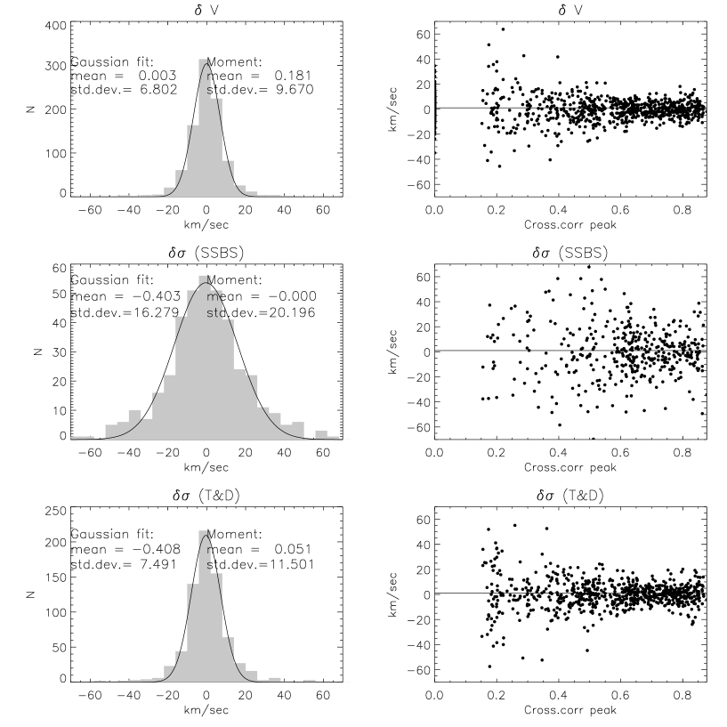
Figure 7: Errors of determination of $v$ (top) and $\sigma$ (in the middle by the SSBS method, at the bottom by the TD method) for the galaxy NGC 2950 over the whole MPFS field of view. The errors were estimated from 4 template stars. The left-hand panels are the histogram of distribution of errors and their Gaussian fit. The right-hand panels show the errors as a function of cross-correlation peak height.

($[n_{o}-\Delta n,n_{o}+\Delta n]$, where $n_{o}$ is the peak location), in which a robust fit with a Gaussian is executed, considering that calibration relation (12) may change for different $\Delta n$.

Obtain a set of coefficients: $\mu(x,y)$, $\alpha_{i}(x,y),\;i=0,1,2$. If the spread of the coefficients from point to point is considerable, it is better to approximate these coefficients along the slit by a second-order polynomial. Construct cross-correlation functions $G(x,y)\otimes T(x,y)$ using relation (9), determine $v$, and from the peak width determine $\sigma$ with the from of (11) and (13) (Fig. 3). One should use here the same value of $\Delta n$ as the one used in construction of calibration relation (12).

To estimate the dispersion by the SSBS method, the right side of expression (15) is approximated with allowance made for the remarks on the choice of the limits $k_{1}$ and $k_{2}$ (see subsection 2.3 and Fig. 5).

By applying the above-described procedure to the spectra of all spatial elements, produce two-dimensional maps of radial velocities $v(x,y)$ and velocity dispersions $\sigma_{TD}(x,y)$, $\sigma_{SSBS}(x,y)$ (the index indicates the method of construction). The heliocentric velocities (reduced to the centre of the Sun) are found from the expression:

$$V_{Hel}=v+V_{*}-V_{\odot,*}+V_{\odot,gal}.$$ (16)

Here $V_{\odot,*}$, $V_{\odot,gal}$ are the heliocentric velocity corrections for the template star and the galaxy computed by the standard method, $V_{*}$ is the radial velocity of a star from the catalogue (reduced to the centre of the Sun).

4.3 Choice of spectral range

The optimum spectral range, in which the analysis described above is made, must contain absorption lines characteristic of the stellar population of galactic nuclei, unblended, when possible. It is desirable that the number of emission lines of ionized gas should be a minimum. Most commonly the regions around the triplets MgI $\lambda\lambda\,5167,5172,5183$ Å  and CaII $\lambda\lambda\,8498,8542,8662$ Å  are used. The latter is more preferable because with one and the same dispersion of the spectrograph the spectral scale (in km/s) in the region of CaII is 1.6 times as large as in the region of MgI. For the advantages of using CaII see the paper by Terlevich et al. (1990).

Unfortunately, the available set of gratings in MPFS made it impossible to work in the region of the infrared triplet CaII without substantial losses of light. Experiments performed in the optical range have demonstrated that the most optimum spectral range to study kinematics of stars at the centres of SO–Sb galaxies is $5100-6100$ Å. It includes strong absorption lines of MgI $\lambda\,5175$ Å, FeI $\lambda\,5229$ Å, FeI+CaI $\lambda\,5270$ Å, NaI $\lambda\,5893$ Å  and others. At the same time, the emission lines are relatively weak and not numerous, noticeable mainly only in Sy galaxies ([NI] $\lambda\,5199$ Å, [FeVII] $\lambda\lambda\,5158,5276,5720,6086$ Å, HeI $\lambda\,5875$ Å). The observations are made with a grating of 1200 gr/mm yielding a reciprocal dispersion of $1.35$ Å/px. The spectral range 4800–6100 Å  contains both the absorption lines described above and the brightest emission lines H_β, [OIII] $\lambda\,4959,5007$, which allows a simultaneous study of ionized gas kinematics.

4.4 Assessment of errors

The assessment of errors in different methods of determination of $\sigma$ and $v$ is considered in some detail in a number of papers (TD, 1979; SSBS, 1977; Larsen et al., 1983). The influence of random and systematic errors is, however, best seen when comparing the results obtained from different template stars during one night. Fig. 7 shows the distribution of errors in the determination of the velocity and velocity dispersion for all 240 individual spectra of NGC 2905 in the MPFS field of view. The mean value for each spatial element was estimated from four stars of spectral classes G7 III–K2 III. The values of the mean errors estimated by the two methods, as the second moment in the distribution of deviations of individual measurements from the mean value over the four stars and as the width of the Gaussian that approximates this distribution, are indicated beside the histograms of the errors. These errors are typical of our observations and make $\delta v=5-10$ km/s for the velocity, $\delta\sigma_{TD}=10-15$ km/s for the velocity dispersion estimated by the cross-correlation technique, and $\delta\sigma_{SSBS}=15-25$ km/s for the Fourier quotient method. For the central regions where the value of the cross-correlation peak is $C_{max}=0.8-1.0$, these errors are about 1.5 times as small as the field average. It can be seen from Fig. 7 that the velocity dispersion errors in the SSBS method increase sharply at $C_{max}<0.7$, that is, one can estimate reliably only the central velocity dispersion. However, since this method requires no additional calibration (subsection 2.3), it is good practice to use the SSBS method estimates for checking the absolute values of the central velocity dispersion.

Figure 8: Comparison of systemic velocities (a) and central velocity dispersions (b) derived from the MPFS observations with the data of the catalogue RC3 and the HYPERCAT database.

We have carried out a number of experiments for testing the precision of the TD and SSBS techniques, using for this purpose the spectra of stars of class G6 III/IV–K3 III obtained with the MPFS. These spectra were artificially smoothed and rendered noisy, then they were employed to estimate the velocity dispersion values. Analysis has shown that if the signal-to-noise ratio in individual spectra is $S/N>20$, it does not affect the accuracy of $\sigma$ determination, which is less than $5-10\%$ of the absolute value of $\sigma$; this is in good agreement with Fig. 7.

The experiments with smoothing have confirmed the well-known fact that it is impossible to reliably determine the velocity dispersion if it is smaller or close to the instrumental profile width. In our case this limit is 70–80 km/s (see Section 3).

The main factor that affects the accuracy of determination of the dispersion for a given S/N and spectral interval are the differences in spectral features of a galaxy and a star which lead to decreasing the contrast of the cross-correlation peak and to differences in the Fourier spectra of the SSBS method. When studying the motions of stars in galaxies of early types, the spectra of red giants G6 III–K3 III are normally used as templates. It is a good idea to take spectra of stars of different spectral classes from this range during one observing night to select a template which is the most close to the galaxy spectrum.

For 8 galaxies observed with the MPFS, we compared our measurements of the systemic velocity (the galaxy centre velocity) with the data of observation of neutral hydrogen velocities in the 21 cm line, which had been taken from the catalogue RC 3 (Fig. 8a). The root-mean-square value of deviations was 17 km/s without a systematic shift. Data on the nuclear velocity dispersion of stars were found in the database HYPERCAT and compared with our estimates (Fig. 8b). No systematic differences are observed; the great scatter of points is most likely due to the fact that only using the 2D technique, one can reliably subtract the spectra from the galaxy dynamical centre.

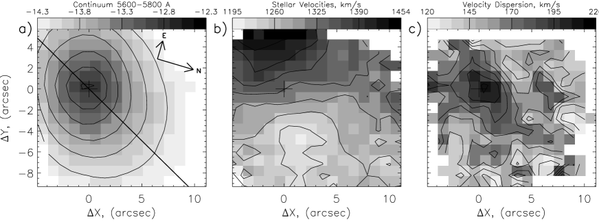
Figure 9: MPFS maps for the galaxy NGC 2950. a — the continuum image (the surface brightness logarithm is in $ergs/cm^{2}/s/\hbox{\hbox to0.0pt{$\sqcap$\hss}$\sqcup$}^{\prime\prime}$), the stright line shows the orientation of the main (outer) bar; b — the velocity field of stars; c — the distribution of the velocity dispersion constructed by the TD method. The origin of coordinates is at the dynamic centre of the galaxy (shown by cross).

5 Example of data reduction: NGC 2950

According to Wozniak et al. (1995) and Friedly et al. (1996) the SB0 galaxy NGC 2950 refers to the so-called double-barred galaxies. In the optical and IR images of the galaxy there is a bar of about $6^{\prime\prime}$ in size inside a $38^{\prime\prime}$ primary bar. The position angles of the bars are $PA=332^{\circ}$ and $272^{\circ}$, respectively. NGC 2950 was observed with the 6 m telescope on March 27/28, 2000 using the spectrograph MPFS, the spectral range was $4820-6200$ Å, the dispersion $1.35$ Å/px, the scale $1^{\prime\prime}$ per lens, the seeing $2^{\prime\prime}$. The total exposure was 3600 s. The field of view of $16^{\prime\prime}\times 15^{\prime\prime}$ covered a region of the inner bar and the central part of the outer bar.

Prior to the continuum subtraction, a smoothing of data was performed in each spectral bin by a Gaussian of $FWHM=1^{\prime\prime}\times 1^{\prime\prime}$ with the aim of optimum filtering of noises. In so doing the spatial resolution decreased slightly and was about 2$.\!\!^{\prime\prime}$3. The further processing was conducted in accordance with Section 4. After the rebinning onto a logarithmic scale, the velocity bin was 50 km/s. Five template stars were taken during the night, 4 of which, yielding a maximum correlation with the galaxy spectrum, were used to construct average velocity fields and velocity dispersion (Fig. 9). When constructing these fields, the points where the error was larger than 20 km/s were masked.

The central velocity dispersion values measured by the TD method ($\sigma=205\pm 5$ km/s) and by the SSBS method ($\sigma=190\pm 10$ km/s) agree with each other and with the data of HYPERCAT ($170\pm 10$ km/s, $182\pm 14$ km/s and $210\pm 14$ km/s from different estimates). The central ellipsoidal structure elongated along $PA\approx 330^{\circ}$, i.e. the one associated with the “outer” bar, is distinguished in the distribution of velocity dispersion (Fig. 9c). At the present time, we continue the work over the study of kinematics of double-barred galaxies; preliminary results are available in the paper by Moiseev and Afanasiev (2001).

6 Conclusions

With the above-described procedure one can construct velocity fields and velocity dispersions of stars in the central parts of early-type galaxies on the basis of data obtained with the spectrograph MPFS. The accuracy of velocity measurement is on the average $\delta v=5-10$ km/s, that of velocity dispersion measurement is $\delta\sigma_{TD}=10-15$ km/s and $\delta\sigma_{SSBS}=15-25$ km/s for TD and SSBS methods, respectively. This technique allows us to take account of the variations of the instrumental profile and produce reliably two-dimensional maps of the velocity dispersion if it is not less than 70–80 km/s. The systemic velocities and the central velocity dispersions that we have measured in 8 S0–Sb galaxies and the HYPERCAT data do not show systematic differences.

We associate the future prospects of studying kinematics of stars in galaxies aided by the spectrograph MPFS with the possibility of observing in the region of the infrared triplet CaII. The accuracy of measurement of velocities and velocity dispersion must in this case be about 1.5–2 times better.

• The author thanks V.L. Afanasiev for formulation of the problem and discussion of results. In the course of work the database HYPERCAT being developed at the Observatoire de Lyon was used.

References

- [1] Afanasiev V.L., Burenkov A.N., Shapovalova A.I., Vlasyuk V.V., 1996, IAU Coll.157, “Barred galaxies”, ASP Conf., 91, Alabama, 218
- [2] Arribas S., Mediavilla E., 2000, “Imaging the Universe in Three Dimensions ”, ASP Conf., 195, 295
- [3] Bottema R., 1988, Astron. Astrophys., 197, 105
- [4] Brault J.W., White O.R., 1971, Astron. Astrophys., 13, 64
- [5] Friedly D., Wozniak H., Rieke M. et al., 1996, Astron. Astrophys. Suppl. Ser., 118, 461
- [6] Gebhardt K., Bender R., Bower G. et al., 2000, Astrophys. J., 539, L13
- [7] Khoperskov A.V., Chulanova E.A, 2001, ”Stellar dynamics: from classic to modern” (Conference, St.Petersburg, 2001), 154
- [8] Larsen N., Norgaard-Nielsen H.U., Kjaergaard P., Dickens R.J., 1983, Astron. Astrophys., 117, 257
- [9] Minkowski R., 1954, Carnegie Yrb., 26
- [10] Moiseev A.V., Afanasiev V.L., 2001, ”Stellar dynamics: from classic to modern” (Conference, St.Petersburg, 2001), 117
- [11] Nelson C.H., Whittle M., 1995, Astrophys. J. Suppl. Ser., 99, 67
- [12] Sargent W.L.W., Schechter P.L., Boksenberg A., Shortridge K., 1977, Astrophys. J., 212, 326 (SSBS)
- [13] Sil’chenko O.K., 1998, Astron. Astrophys., 330, 412
- [14] Terlevich E., Diaz A.I., Terlevich R., 1990, Mon. Not. R. Astron. Soc., 242, 271
- [15] Tonry J., Davis M., 1979, Astron. J., 84, 1511 (TD)
- [16] Wozniak H., Friedli D., Martinet L. et al., 1995, Astron. Astrophys. Suppl. Ser., 111, 115