Searching and studying clusters with the SZ effect

Abstract

I discuss galaxy cluster surveys based on the Sunyaev–Zel’dovich effect and their relevance for cosmological studies. The unique aspects of cluster selection by this method are emphasized and certain issues of surveying are addressed. Finally, I briefly present prospects for upcoming surveys.

Observatoire Midi–Pyrénées, Toulouse, France
New institution: APC – Université Paris 7, Paris, France

1. Introduction

Galaxy cluster catalogs are useful for cosmological studies for a number of reasons: cluster abundance, distribution and evolution reflect the structure formation process, which depends sensitively on certain cosmological parameters, such as the matter density $\Omega_{\rm M}$ (Oukbir & Blanchard 1992, 1997; Bahcall 1998; Bartlett 1997; Borgani et al. 1999 & these proceedings; Eke et al. 1998; Henry 1997; Viana & Liddle 1999); and cluster internal properties provide clues to the nature of dark matter and on certain mechanisms associated with galaxy formation, such as heating and feedback.

The construction of well–defined catalogs appropriate for statistical studies demands good understanding of the cluster selection criteria (see Postman, these proceedings). These criteria in turn depend on the type of observations – optical, X–ray, radio – as well as on the data analysis proceedures. Each type of observation has its own advantages and disadvantages that we may refer to as its intrinsic biases. For example, X–ray cluster selection eliminates the problem of projection effects suffered by optical observations, but on the other hand is significantly influenced by the rather poorly understood physics taking place in the core region.

The question that arises is, what kind of selection is best? The answer clearly depends on the utlimate use of the catalog, and for cosmological studies we may argue that the most ideal selection would be based on cluster mass. This is because cluster mass and redshift are the two primary theoretical cluster descriptors. From this line of argument, understanding cluster selection criteria is reduced to relating the observational selection criteria to cluster mass and redshift. This is a useful viewpoint, for it provides a framework for quantifying the biases associated with each type of observation for the purposes of cosmological studies. We do not argue that one particular observational method is the best; rather, that the important point is to use several methods with different biases.

The Sunyaev–Zel’dovich (SZ) effect (Sunyaev & Zel’dovich 1972) will soon open the way to a new method of surveying for clusters. Several ground–based instruments optimized for SZ surveying are currently under construction, and the Planck satellite will supply an almost full–sky catalog of several $10^{4}$ clusters at the turn of the decade. In anticipation and in the spirit just outlined, we shall now examine in more detail this new kind of survey (the ‘SZ band’), and in particular the nature of its cluster section.

This potential of surveying for clusters with the SZ effect has been appreciated for some time. To my knowledge, the first to give source count predictions were Korolyov, Sunyaev, & Yakubstev (1986), and many authors have since considered the issue. An indicative, useful, though by no means exhaustive, list of references focused on SZ surveying (i.e, counts and redshift distributions of SZ detected clusters) would include: Bond & Meyers (1991), Bartlett & Silk (1994), Markevitch et al. (1994), Barbosa et al. (1996), Eke, Cole, & Frenk (1996), Aghanim et al. (1997), Colafrancesco et al. (1997), da Silva et al. (2000), Holder et al. (2000), Lo et al. (2000), Benson, Reichardt, & Kamionkowski (2001), Fan & Chuieh (2001), Kay, Liddle, & Thomas (2001), Kneissl et al. (2001), Springel, White, & Hernquist (2001), Xue & Wu (2001).

2. SZ Cluster Selection

In the non–relativistic limit (which applies in practice to all but the hottest clusters), the SZ effect may be written as

$$\delta i_{\nu}(\hat{n}) = y(\hat{n})j_{\nu}$$

$$y = \int_{los}\frac{kT}{mc^{2}}n\sigma_{T}dl$$

where $\delta i_{\nu}$ is the brightness change induced in the cosmic microwave background (CMB) by compton scattering off electrons (mass $m$) in the hot intracluster medium (ICM) at temperature $T$ and electron density $n$. The Compton $y$–parameter measures the amplitude of the energy transfer to the photons ($\sigma_{T}$ is the Thompson cross section); and the function $j_{\nu}$ describes the spectral form of the distortion. It is convenient to consider the effect integrated over the entire cluster face:

$$Y=\int d\Omega\;y(\hat{n})\propto f_{\rm gas}\frac{M\langle T\rangle}{D_{\rm ang}^{2}}$$ (1)

where now $M$ is the cluster (virial) mass, $f_{\rm gas}$ is the ICM gas mass fraction, $\langle T\rangle$ is the (true) mean electron temperature (i.e., particle weighted), and $D_{\rm ang}(z)$ is the angular–size distance. Notice that $Y$ is measured in, for instance, square arcmins.

It is from these equations that we begin to understand the nature of SZ cluster selection (or detection). Let us emphasize four aspects:

1. The spectral signature $j_{\nu}$ is unique – negative at low frequency, positive at high frequency, with a fixed zero point at $\lambda\sim 1.4$ mm – and the same for all clusters ($j_{\nu}$ depends only on the observation frequency). There is therefore no k–correction;

2. The integrated effect $\propto D_{\rm ang}^{-2}$, which is the statement that the surface brightness is independent of redshift $z$. This is in contrast to other emission mechanisms, that vary as the luminosity distance $D_{\rm lum}=(1+z)^{2}D_{\rm ang}$, and which suffer from ‘cosmic dimming’ (the redshift);

3. The integrated signal is directly proportional to the total ICM thermal energy $f_{\rm gas}M\langle T\rangle$ (this is essentially the definition of the mean temperature $\langle T\rangle$). We may therefore expect a tight correlation between the measurable, $Y$ and the cluster mass, e.g., $Y\propto f_{\rm gas}M^{5/3}$, especially in the more massive systems where non–graviational effects appear less important.

4. Cluster detection and subsequent modeling may be based on the same measurable quantity $Y$.

A particularily useful quantity for characterizing the selection properties of a survey is the minimum detectable mass as a function of redshift, $M_{\rm det}(z)$. For example, it determines the source counts as

$$\frac{dN}{d\Omega}=\int_{0}^{\infty}dz\;\frac{dV}{dzd\Omega}\;\int_{M_{\rm det}(z)}^{\infty}dM\;\frac{dn}{dM}(M,z)$$ (2)

where $dn/dM$ is the mass function. A comparison of $M_{\rm det}$ from all–sky X–ray and SZ (the Planck curve) surveys is made in Figure 1. The X–ray survey flux limit corresponds to that of the RASS. An interferometer–like similar to those proposed (see below) and capable of surveying several square degrees from the ground is also shown. To make the figure, a non–evolving $L_{x}-T$ relation of the form given by Arnaud & Evrard (1999) and a $T-M$ relation from Evrard, Metzler, & Navarro (1996) have been adopted. The cosmological model is an open, low–density model, and Eq. (1) was used with a constant gas mass fraction $f_{\rm gas}=0.06h^{-1.5}$ (Evrard 1997)

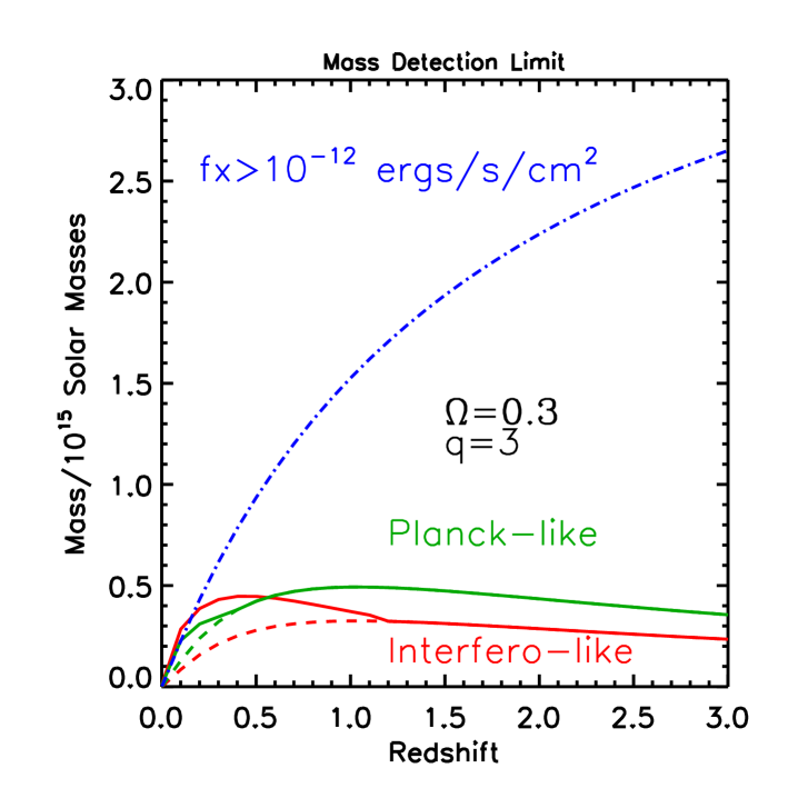
Figure 1.: Minimal detectable mass as a function of redshift for a Planck–like all–sky survey, an interferometer–like (limited sky, ground–based) survey and for a flux–limited X–ray survey similar to the RASS. For the SZ curves, the dashed lines account for cluster extension, while the solid lines assume that clusters are point sources. The Planck–like survey is based on the Planck 2.1 mm channel performance only: $Y=10^{-4}$ arcmin²/beam and an angular resolution of $\theta_{\rm fwhm}=5$ arcmins (this is most surely an optimistic estimate as the Planck SZ maps will be weighted by channels with differing resolution and sensitivity, and foreground removal will further degrade the sensitivity). The interferometer–like curve assumes $\theta_{\rm fwhm}\sim 2$ arcmin and a sensitivity of $Y=5\times 10^{-5}$ arcmin².

The figure is illustrative, especially because we have no idea of the evolution of the $L_{x}-T$ relation to such redshifts. It is nevertheless instructive to note the different behavior of the X–ray and SZ curves, and in particular the almost flat asymptote of the SZ curves; in fact, they demonstrate a slow decrease towards high redshift (this is independent, of course, of the $L_{x}-T$ relation). In other words, SZ selection corresponds essentially to a mass selection. The conclusion depends in detail on the constancy of $f_{\rm gas}$ with redshift, but the potential consequences are interesting: for example, this implies that there is no $V_{\rm max}$ for a SZ detected cluster. Even more significant is that SZ selection therefore finds the same kinds of objects (mass–wise) over a large range of redshifts. For evolutionary studies of clusters, this is an important advantage over other selection techniques that force one to compare ever more massive objects detected at high redshift to less massive local samples.

3. Aspects of Surveying

The discussion so far as assumed that clusters are unresolved – that the integrated SZ flux of Eq. (1) is directly measured. This situation applies in practice to the Planck survey, with angular resolution of at best 5 armins. Ground–based instruments, on the other hand, will operate at higher resolution and clusters will appear extended, complicating the selection criteria: some clusters may be resolved out, relative to a hypothetical point–source approximation. Detection depends now not only on $Y$, but also on the detailed SZ cluster profile; and photometry becomes an issue, as with any extended source.

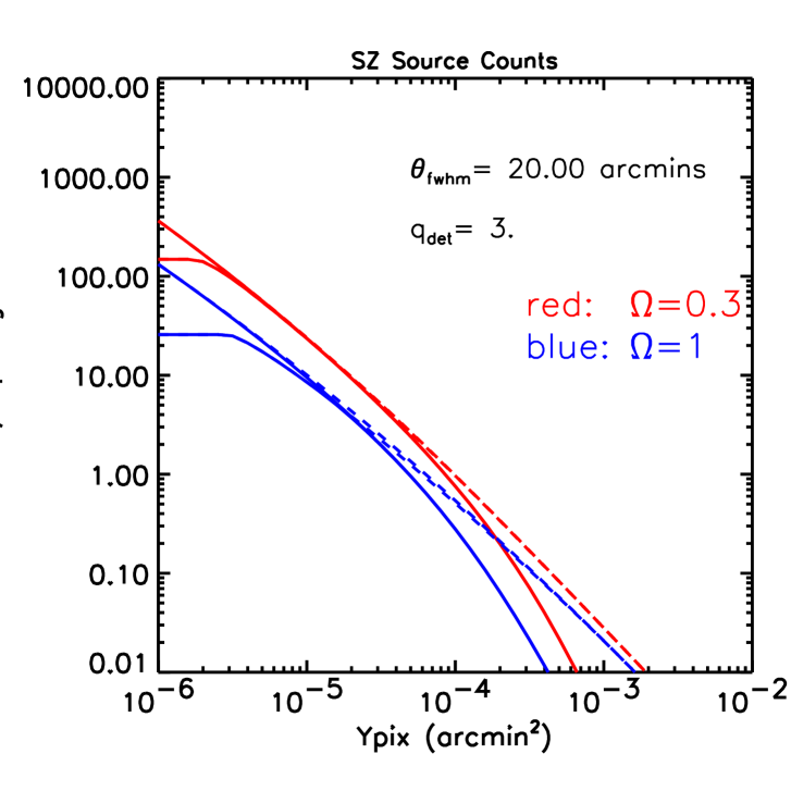
Figure 2.: Integrated SZ counts as a function of pixel noise expressed in terms of $Y$ (arcmin²). Two cosmological models are used to illustrate the effects of source extension. The upper (red) curves are for an open model and the lower (blue) curves are for a critical model. The solid curves take into account finite source extension with a simple analytical model (Bartlett 2000), while the dashed lines give the results of the point–source approximation. In all cases, two different low–mass cutoffs – $10^{13}$ & $10^{14}$ solar masses – are applied in order to highlight the contribution of low–mass objects. The effect of the latter cutoff is clearly seen as the point where the counts flatten off at low $Y$.

Many ground–based instruments will operate, at least at first, at a single frequency. In this case, primary CMB fluctuations (in the background) become an important source of noise, and one must extract extended sources over a fluctuating background. Another potentially important effect is confusion by point sources, either randomly distributed on the sky, or preferentially in cluster cores. Without spectral information, their removal requires higher resolution imaging; for this reason, some ground–based interferometer projects plan to control this confusion with additional telescopes placed on long baselines.

There are certainly other issues, for example other foregrounds, that we could list as problematic. However, I would instead like to address a specific question that often arises when preparing a survey: In a given amount of observing time, should one go (integrate) ‘deep’, or instead ‘wide’, covering more sky to less depth? Actually, the real approach is to try to do several surveys, i.e., in some sense to do both. All the same, it is useful to try to answer the question in terms of maximizing the number of detected objects. This depends on the slope of the source counts as a function of survey sensititivity.

3.1. Deep or Wide?

We calculate the counts using Eq. (2). For unresolved sources, the detection mass is only a function of sensitivity, $Y_{\rm noise}$, and redshift – $M_{\rm det}(Y_{\rm noise},z)$. Additional factors are important in the case of resolved source detection, such as angular resolution ($\Omega_{\rm pix}$, the solid angle of a ‘pixel’) and source profile: $M_{\rm det}(Y_{\rm noise},z,\Omega_{\rm pix},profile)$. A simple analytic model of extended source detection in a map may be employed to examine cluster selection (Bartlett 2000). It supposes that one can identify and then integrate over all the pixels covering a cluster (out to the virial radius) to access the total cluster signal $Y$ for detection; it is therefore the best one can hope to do.

Using this approach, the effects of resolution on $M_{\rm det}$ are presented in Figure 1, where the dashed lines (for the SZ curves) give $M_{\rm det}(z)$ once cluster extension has been taken into account. Clearly, clusters at low/intermediate redshifts are resolved out relative to the point–source calculation, because they are covered by several noisy pixels; this is most evident for the higher resolution interferometer–like curve. The difference for a low resolution survey, such as the Planck survey, is relatively minor, as can been seen.

This point is important when it comes to predicting the number of objects to be expected. Clearly the predicted number will be lower when correctly accounting for resolution effects. Even more relevant to the question at hand (deep or wide), is the fact that, as seen in Figure 2 (and in Figure 4 below), the actual counts as a function of sensitivity are steeper than the point–source calculation would suggest. In fact, at the bright end they are steeper than $Y_{\rm noise}^{-2}$, the critical slope for answering our question. Counts steeper than $-2$ imply that more objects will be found by integrating deep on a small patch of sky (as long as $Y_{\rm noise}\sim t^{-1/2}$, which usually applies). At the faint end, the counts flatten out and rejoin the point–source calculation, which is always flatter than $Y_{\rm noise}^{-2}$. Two important conclusions follow:

1. the point–source calculation gives the wrong answer in suggesting that one should go wide;

2. the correct answer is found by accounting for resolution effects and indicates that, for each experimental set–up, there is an optimal sensitivity corresponding to the point where the counts reach a slope of $-2$.

4. Expectations

A number of dedicated instruments optimized for SZ surveying have recently been proposed. At the time of writing, many of these projects are funded and under construction, including:

• Interferometer arrays

  • Arcminute MicroKelvin Imager (AMI)
    (http://www.mrao.cam.ac.uk/telescopes/ami/index.html)

  • Array for Microwave Background Anisotropy (AMiBA)
    (http://www.asiaa.sinica.edu.tw/amiba/)

  • SZ Effect Imaging Array
    (http://www.astro.uiuc.edu/ jmohr/SZE/index.html)

• Bolometer cameras

  • ACBAR
    (http://cfpa.berkeley.edu/ swlh/research/acbar.html)

  • BOLOCAM
    (http://www.astro.caltech.edu/ lgg/bolocam/bolocam.html)

• Planck satellite
  (http://astro.estec.esa.nl/Planck/)

Several authors have recently made predictions for these various instruments (Aghanim et al. 1997; Holder et al. 2000; Lo et al. 2000; Benson et al. 2001; Kay et al. 2001; Kneissl et al. 2001). In Figures 3 & 4 I show some expectations for the Planck Survey and for the AMI interferometer, both for two extreme cosmologies: a critical model and a purely open model with $\Omega_{\rm M}=0.3$. A flat low–density model with non–zero cosmological constant will fall between these two cases, although somewhat closer to the purely open model.

In the following, it should be kept in mind that the predicted total number of detected clusters is subject to large modeling uncertainties and can vary by as much as a factor of $\sim 5$. A particularly important source of uncertainty comes from the uncertainty in the amplitude of the density perturbations $\sigma_{8}$. To be conservative, the predictions are given for ‘low $\sigma_{8}$’: $(\sigma_{8}=0.8,\Omega_{\rm M}=0.3)$ and $(\sigma_{8}=0.5,\Omega_{\rm M}=1)$ (e.g., Eke et al. 1998). Use of higher values quoted in the literature (e.g., Blanchard et al. 2000; Pierpaoli, Scott, & White 2001) would substantially increase the predicted total number of clusters. Another source of uncertainty lies in the potential evolution of the cluster gas mass fraction $f_{\rm gas}$. The lack of evidence for strong evolution of $f_{\rm gas}$ with redshift or for an important dependence on cluster mass may simply reflect a lack of sufficient data. In this light, it is important to note that the SZ signal for unresolved clusters (e.g., Planck detections) depends only on the global quantity $f_{\rm gas}$, and not on the details of the gas distribution; X–ray observations, as a contrast, are heavily influenced by the physics of the core, which is very poorly understood and difficult to model.

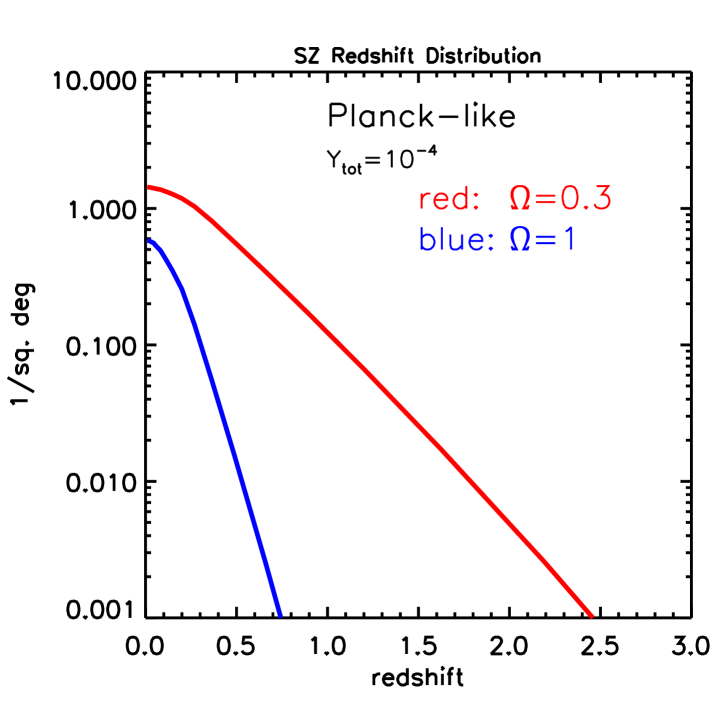
Figure 3.: Planck–like cumulative redshift distributions for two extreme cosmologies. The $y$–axis gives the counts at $Y>10^{-4}$ arcmin² for objects at redshifts $>z$, plotted as a function of $z$ ($x$–axis). The upper (red) curve corresponds to the open model, while the lower (blue) curve is for the critical model. In addition to the various modeling uncertainties mentioned in the text, the predicted number of clusters depends on the final sensitivity of the survey, which for the fixed observing time of the mission will depend on various factors, including the weighting given to each of the bands, the effects of foreground removal, etc… This is an area of current study.

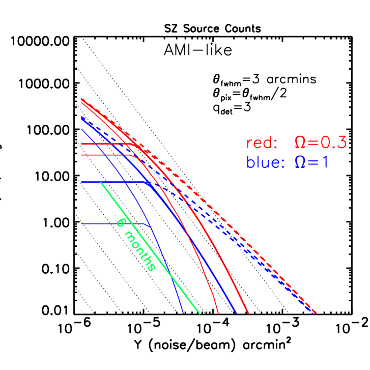
Figure 4.: Integrated counts for an AMI–like instrument as a function of survey sensitivity in terms of noise rms/beam. The color code is the same as above. The thick solid lines show the total counts, while the thin solid lines show only unresolved sources. Each model is plotted for two different low–mass cutoffs ($10^{13}$ and $10^{14}$ solar masses); the higher mass cutoff in each case can be seen to flatten off at the low–noise end. The dashed lines show the results of the (invalid) point–source approximation, for both mass cutoffs and for the open model (above) and the critical model (below). Finally, the dotted lines in the background indicate the critical slope of $-2$, steeper than which deep surveys yield more objects than wide, shallow ones.

The Planck predictions are given in terms of redshift distributions: shown as a function of redshift $z$ are the total number of clusters with $Y>10^{-4}$ armin² at redshifts larger than $z$. The numbers at $z=0$ therefore give the total number of detectable clusters, and we see that on the order of 1 cluster/sq.deg. is expected for the survey, depending on the cosmology. At $z\sim 1$ the two models differ wildly. There are essentially no clusters expected in the critical model. On the other hand, about 10% of clusters are expected to lie at $z>1$ in the open scenario. These conclusions assume that $f_{\rm gas}$ remains relatively constant with redshift and mass. The presence of an important population of clusters at high redshift would be a strong indication of a low–density universe; but the lack of such a population could be accommodated in the open model by decreasing $f_{\rm gas}$ with $z$. The result in any case would be an important piece of cosmological information.

The predictions for an AMI–like instrument (resolution of a few arcminutes or better) are given in terms of integrated source counts as a function beam sensitivity. Both cosmological models are once again shown, each one for two different low–mass cutoffs ($10^{13}$ and $10^{14}$ solar masses) in order to separate the contribution of low and high mass objects. The dashed curves show the equivalent counts in a point–source approximation, and we observe that the latter fails rather badly because most clusters are resolved at this resolution. The dotted lines in the background follow the critical slope of $Y^{-2}$. This kind of instrument reaches its optimal sensitivity at $\sim few\times 10^{-5}$ arcmin²/beam, where the predicted counts attain a slope of $-2$. At this sensitivity, one may expect, as a conservative round number and within the modeling uncertainties mentioned, on the order of several clusters/sq.deg.

5. Conclusion

It will shortly be possible to perform purely SZ–based surveys, opening up what may be refered to as the ‘SZ band’ for cluster studies. A number of ground–based instruments will realize such surveys within a few years over patches of sky covering several square degrees; and by the end of the decade, the Planck mission will produce a catalog of several $10^{4}$ SZ clusters over the majority of the sky. Although predictions for the number of clusters expected for these surveys suffer from modeling uncertainties, various studies indicate roughly on the order of $\sim 1$ cluster/sq.deg. for Planck and $\sim few$ clusters/sq.deg. for the deeper ground–based efforts under way.

These surveys represent a new method for studying clusters that will find its place alongside X–ray and optical methods. As a population, clusters provide a unique statistical sample for probing cosmology and the large–scale structure formation process. Each observational approach to surveying for clusters has its proper advantages and disadvantages (collectively, its biases). In light of cosmological studies, it is most instructive to quantify observational biases in terms of cluster mass and redshift, the two primary theoretical cluster descriptors. The specific advantages inherent to SZ surveying are listed above under Section 2 and include the fact that the integrated SZ signal is proportional to a physical quantity – the ICM thermal energy.

For a more complete understanding of the cluster population in view of its application as a cosmological probe it is essential to combine a variety of surveying (catalog selection) methods with different biases. SZ surveying will soon add an important new, independent and complementary approach in this endeavor.

I would like to thank the organizers for their invitation to a most interesting and enjoyable meeting.

References

Aghanim, N., de Luca, A., Bouchet, F.R., Gispert, R., & Puget, J. L. 1997, A&A, 325, 9

Arnaud, M., & Evrard, A.E. 1999, MNRAS, 305, 631

Bahcall, N., & Fan, X. 1998, ApJ, 504, 1 &

Barbosa, D., Bartlett, J.G., Blanchard, A., & Oukbir, J. 1996, A&A, 314, 13

Bartlett, J.G. 1997, in ASP Conf. Ser. Vol. 126, From Quantum Fluctuations to Cosmological Structures, ed. D. Valls–Gabaud et al. (San Francisco: ASP) 365

Bartlett, J.G. 2000, astro–ph/0001267

Bartlett, J.G., & Silk, J. 1994, ApJ, 423, 12

Benson, A.J., Reichardt, C., & Kamionkowski, M. 2001, astro–ph/0110299

Blanchard, A., Sadat, R., Bartlett, J.G., & Le Dour, M. 2000, A&A, 362, 809

Bond, J.R. & Meyers, S.T. 1991, in Trends in Astroparticle Physics, ed. D. Cline (Singapore: World Scientific)

Borgani, S., Rosati, P., Tozzi, P., & Colin, N. 1999, ApJ, 517, 40

Colafrancesco, S., Mazzotta, P., Rephaeli, Y., & Vittorio, N. 1997, ApJ, 433, 454

da Silva, A.C., Barbosa, D., Liddle, A.R., & Thomas, P.A. 2000, MNRAS, 317, 37

Eke, V.R., Cole, S., & Frenk, C.S. 1996, MNRAS, 282, 263

Eke, V.R., Cole, S., Frenk, C.S., & Henry, P.J. 1998, MNRAS298, 1145

Evrard, A.E. 1997, MNRAS, 292, 289

Evrard, A.E., Metzler, C.A., & Navarro, J.F. 1996, ApJ, 469, 494

Fan, Z. & Chiueh, T. 2001, ApJ, 550, 547

Henry, J.P. 1997, ApJ, 489, L1

Holder, G.P., Mohr, J.J., Carlstrom, J.E., Evrard, A.E., & Leitch, E.M. 2000, ApJ, 544, 629

Kay, S.T., Liddle, A.R., & Thomas, P.A. 2001, MNRAS, 325, 835

Kneissl, R., Jones, M.E., Saunders, R., Eke, V.R., Lasenby, A.N., Grainge, K., & Cotter, G. 2001, astro–ph/0103042

Korolyov, V.A., Sunyaev, R.A., & Yakubtsev, L.A. 1986, Sov. Astron. Lett., 12, L141

Lo, K.Y., Chiueh, T.H., Martin, R.N., Kin–Wang Ng, Liang, H., Ue-li Pen, & Chung-Pei Ma 2000, astro–ph/0012282

Markevitch, M., Blumenthal, G.R., Forman, W., Jones, C., & Sunyaev, R.A. 1994, ApJ, 426, 1

Oukbir, J., & Blanchard, A. 1992, A&A, 262, L21

Oukbir, J., & Blanchard, A. 1997, A&A, 317, 1

Pierpaoli, E., Scott, D., & White M. 2001, MNRAS,325, 77

Springel, V., White, M., & Hernquist, L. 2001, ApJ, 549, 681

Sunyaev, R.A. & Zel’dovich, Ya.B. 1972, Comm. Astrophys. Space Phys., 4, 173

Viana, P.T.P., & Liddle, A.R. 1999, MNRAS, 303, 535

Xue, Y.–J., & Wu, X.–P. 2001, ApJ, 552, 452