CMB and Inflation: the report from Snowmass 2001

Abstract

Astrophysical observations provide the best evidence of physics beyond the particle physicists’ standard model. Over the past decade, the case has solidified for inflation, dark energy, dark matter and massive neutrinos. In this report we focus on inflation and dark energy as constrained by the CMB—first the evidence from current observations and then what we can expect to learn in the future. High energy physicists can contribute to the succesful realization of this future, both observationally and theoretically.

I Introduction

Accelerator–based efforts spanning decades have revealed no direct evidence of physics beyond the Standard Model. Although this is likely to change with the Large Hadron Collider (LHC) or possibly even with the current (higher–luminosity) run at the Tevatron, we point out that astrophysical evidence for physics beyond the standard model has already grown to be conclusive. Observations indicate the need for

• inflation,

• dark energy,

• dark matter, and

• massive neutrinos.

In short, cosmology is delivering on its promise of probing fundamental physics.

These results are creating intellectual excitement in the high energy physics community. They also signal an opportunity. The prospects are bright for further progress in our understanding of fundamental physics, via cosmology, and researchers trained in particle physics should not only be interested, but are well–equipped to contribute. Indeed, a number of particle physicists have become actively engaged in astrophysical observations.

In this report we review the current status of observations of the temperature of the cosmic microwave background (CMB), and explain how they provide evidence of an inflationary era of expansion in the early Universe and the existence of “dark energy”. One of our intentions in providing this review is to demonstrate that cosmology has a track record which suggests that we have some understanding of the system we are studying. This track record bolsters the case that we will be able to get meaningful answers to the more detailed questions that are motivating planned observations. These future observations, which we discuss, include more detailed measurement of temperature maps, detection and measurement of polarization (including the modes generated by gravitational waves) and Sunyaev–Zeldovich surveys. Of course, observational cosmology is much broader than the topics we are covering, and the interested reader is encouraged to consult the other P4 and E6 subtopic reports.

II Overview of CMB and Fundamental Physics

Observations of the CMB are powerful probes of physical processes in the early Universe. This is due to the richness of the observables and the relative ease with which they can be calculated from first principles. The CMB may be unique in astrophysics in that its properties, over a wide range of angular scales, can be accurately predicted for a given model in linear perturbation theory.

The CMB is most importantly a probe of structure formation in the Universe. The past decade has confirmed that structure in the Universe grew from highly–uniform initial conditions (density fluctuations of order 1 part in $10^{5}$) via gravitational instability. The evolution of these initial perturbations is sensitive to a number of cosmological parameters, including the mean curvature, density of baryons, density of cold dark matter, density of hot dark matter, density of dark energy, and the epoch of reionization of the IGM. Observations of CMB anisotropy are thus sensitive to these parameters and, in addition, the statistical properties of the initial conditions.

We do not expect these “initial conditions” to be genuinely initial but rather the result of some dynamical process. The CMB is already providing us strong evidence that this generation occurred during an inflationary stage in the expansion of the Universe. The fundamental physics responsible for inflation is far from being understood, although there is no dearth of toy models. The possible energy scale of this phenomenon ranges from $10^{3}$ GeV up to $10^{16}$ GeV.

The applicability of linear perturbation theory is due to the fact that the microwave background photons last interacted with matter at a redshift of $z\simeq 1100$ when the perturbations were still well in the linear regime. We can probe structure at this epoch by making maps of the intensity of the CMB (or, equivalently its temperature) and also of the polarization. We have already learned much from temperature maps (to be summarized below) and expect the first detections of polarization within the next one to two years. We expect high sensitivity, high angular resolution maps of temperature and polarization to provide strong constraints on models of inflation, and high–precision constraints on cosmological parameters.

High–sensitivity polarization maps may actually allow us to determine the energy scale of inflation. Although both scalar (density) perturbations and tensor (gravitational wave) perturbations to the metric tensor result in curl–free polarization patterns, only the tensor perturbations result in non–zero curl. Detection of curl in the polarization pattern (sometimes referred to as the “B mode”) would be evidence for gravitational waves and their amplitude is directly proportional to the energy–scale of inflation. Detecting the B–mode is a very challenging task, probably requiring large–scale dedicated detector arrays (either ground or space–based). We consider succesful detection of this signal to be very exciting but a long shot. Further observations will shed light on our chances of success.

Observations of the last–scattering surface do not provide strong constraints on the nature of the dark energy (such as its density today, and equation of state). Fortunately, not all CMB photons arrive at us today undisturbed by matter along the line–of–sight. Some pass through rich clusters of galaxies whose hot electrons scatter them to higher energies, creating a spectral distortion called the Sunyaev–Zeldovich (SZ) effect. Since the number density of clusters is sensitive to the dark energy density and equation of state, SZ surveys can tell us about these quantities. Gravitational lensing of the CMB and the “Rees–Sciama” effect also create anisotropies at late times with statistical properties that are sensitive to the nature of the dark energy.

To summarize this overview, there are three observable properties of the CMB which all provide unique constraints on particle physics models. These are the spectrum (observed to be that of a black body, except in the direction of clusters of galaxies), temperature anisotropy, and polarization. In Sections III and IV we review the physics probed by the CMB, and in Section V we report on the current status of temperature and polarization measurements. In section VI we discuss the future of CMB temperature and polarization measurements, in section VII we discuss the challenges of analyzing the large data sets expected from future experiments, and in section VIII we review the ways in which SZ surveys probe cosmological parameters, including dark energy.

III Inflation and Perturbation Generation

There is a large literature on inflation. We give a very brief treatment here and point the reader to some recent reviews linde00 ; guth00 .

For spatially flat models, the expansion rate and its rate of change are given by

$$H\equiv{\dot{a}\over a}=\sqrt{8\pi G\rho\over 3}\ \ ;\ \ {\ddot{a}\over a}=-{4\pi G\over 3}\left(\rho+3P\right).$$ (1)

Thus acceleration of the scale factor, the essence of inflation, requires $P<-\rho/3$.

Inflation is often modeled as being driven by the vacuum energy of a spatially homogeneous scalar field, $\phi$. The dynamics of this scalar field are usually calculated classically, by use of an effective potential to account for the quantum–mechanical radiative corrections, $V(\phi)$. The equation of motion for this scalar field in an expanding Universe is then

$$\ddot{\phi}+3H\dot{\phi}+V^{\prime}(\phi)=0$$ (2)

and the energy density and pressure are:

$$\rho = V(\phi)+\dot{\phi}^{2}/2$$

$$P = -V(\phi)+\dot{\phi}^{2}/2$$ (3)

Inflation occurs when $\dot{\phi}^{2}/2<<V(\phi)$ so that $P\simeq-\rho$.

Perturbations are generated quantum–mechanically. In de Sitter space, all massless scalar fields have fluctuations with rms amplitude $\delta\phi=H/(2\pi)$ on the horizon scale. The resulting density perturbations are the initial seeds of structure. There is a short and simple treatment of the generation and evolution of these density perturbations in linde00 . For a more in depth treatment see mukhanov92 .

The perturbations in the scalar field result in scalar metric perturbations (i.e., they transform like scalars under spatial rotations). Inflation also produces tensor perturbations to the metric, which are gravitational waves. Unlike the scalar perturbations (which are also sensitive to $\partial V(\phi)/\partial\phi$) the tensor perturbation amplitude depends only on the expansion rate during inflation, and thus almost solely on $V(\phi)$. Detection of these tensor perturbations is necessary for a determination of the energy scale of inflation.

Inflation faces some conceptual challenges. For one, the vacuum energy of the scalar field plays a central role, even though we do not understand the cosmological constant problem. Secondly, we have used an effective potential description which is derived assuming the scalar field is in a stationary, equilibrium state to describe dynamics of the scalar field. Although there has been no progress with the first problem, there has been some with the second. Quantum corrections to the classical treatment of the evolution of the mean value of the scalar field, implicit in use of the effective potential, are only important for potentials with negative curvature, $\partial^{2}V(\phi)/\partial\phi^{2}<0$. Even for these models though, the evolution can be treated in the same classical manner, but with the tree-level potential replaced by an effective one with two scalar fields. cormier99

Inflation can arise from very simple potentials, including $V(\phi)\propto\phi^{n}$ for $n>1$. In Figure 1, reproduced from dodelson97 , we show predictions from a variety of potentials in the plane of power spectrum parameters, $n$ and $r$ where $n$ is the power–law spectral index for the primordial scalar power spectrum, $P(k)=Ak^{n}$ and $r\equiv T/S$ where $T$ is the tensor contribution to the quadrupole anisotropy variance $C_{2}$ and $S$ is the scalar contribution. Also shown are forecasted error ellipses from expected MAP and Planck data. Thus it is clear that precisions measurements of the CMB can lead to great power in distinguishing among inflationary models.

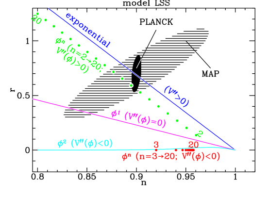
Figure 1: Predictions for a range of models in the $n$ and $r$ plane and forecasted error ellipses from expected MAP and Planck data (from dodelson97 ).

IV Physics of Acoustic Oscillations

After an epoch of inflation, the evolution of the particle species present in the Universe and of perturbations to densities of those species is well understood. Here we present a very brief review of this evolution and the imprint left on the photons that will become the CMB we observe today. It recaps material presented at greater length and detail in textbooks (e.g., KolbTurner ; Peebles ) and review articles (e.g., HuScoSil94 ).

After Big-Bang Nucleosynthesis, the Universe is composed of relativistic species (photons and neutrinos, with density $\Omega_{r}$), baryons in the form of light nuclei ($\Omega_{B}$), and dark matter ($\Omega_{c}$). At temperatures higher than about one eV, the nuclei remain ionized, and the photons and baryons are tightly coupled in a plasma. As the Universe cools, the electrons and baryons very rapidly combine to form (mostly hydrogen) atoms, and the photon mean-free-path grows to be larger than the scale of the Universe (the Hubble length) at this time, known as “Last Scattering,” “Matter-Radiation Decoupling,” and “recombination” (although technically these terms refer to slightly different events, they all occur at roughly the same epoch, at a temperature of $\sim 1$eV or a redshift of $z\simeq 1,100$ or an age of about 300,000 years. [This is considerably below the naive expectation of 13.6eV due to the overwhelming number of photons compared to baryons—a factor of $\sim 10^{10}$—keeping the latter ionized longer.] Free-streaming through the Universe since this time, these same photons redshift to become the 2.728K CMB observed today.

The early Universe was highly homogeneous with small density perturbations, $\delta\equiv\delta\rho/\rho$ in the various components with density $\rho$. As discussed above, Inflation is at the moment the best—and perhaps the only—way of creating these fluctuations. The accelerated expansion makes the Hubble length grow much more slowly than the past horizon, allowing for the causal creation of fluctuations with wavelengths much larger than the Hubble length.

The simplest inflationary models create perturbations where the fractional perturbations are the same in all species. Since the per-particle entropy is therefore spatially constant, such perturbations are refererred to as “adiabatic”. More complicated models can also produce isocurvature perturbations, in which density fluctuations in some species are initially exactly compensated by density fluctuations in other species. The data are consistent with pure adiabatic and inconsistent with (at least the simplest) pure isocurvature models. Inflation also generically leads to Gaussian, statistically isotropic perturbations whose statistical properties are completely described only by a correlation function or, in three-dimensional Fourier space, a power spectrum, $P(k)$. Typically what is assumed in comparing CMB data with models is that there is an initially adiabatic set of perturbations with power spectrum parameterized by an amplitude and power–law spectral index, $n$.

When the scale of a density perturbation is greater than that of the Hubble length, the nature of the separate components (dark matter, photons, baryons) is irrelevant. However, because of their different equations-of-state and different inter–species interactions, the small-scale dynamics of perturbation evolution is different for the various components. When the Universe has aged sufficiently that a wave of some given size is of a scale comparable to the Hubble length (we casually say that the scale has “entered the horizon”), pressure and gravitational potential gradients become important. These gradients drive sound waves in the multi-component plasma. An important length scale for this dynamical process is the sound horizon, the distance a sound wave could have travelled since the Big Bang. Because the Universe has been dominated by radiation (with sound speed $c/\sqrt{3}$) for most of its history, the sound horizon is about ($1/\sqrt{3}$) of the (classical Big Bang) particle horizon.

First, consider waves entering the (sound) horizon around the time of last scattering: these are the largest waves that could have formed a coherent structure at this time. Indeed, by determining the characteristic angular scales of the CMB fluctuation pattern, and matching this to the physical scale of the sound horizon at last scattering we can determine the angular diameter distance to the last scattering suface, which is mostly dependent on the geometry of the Universe: in a flat universe, angular and physical scales obey the usual Euclidian formulae; in a closed (positively curved) universe, geodesics converge and a given physical scale corresponds to a larger angular scale (and hence smaller multipole $\ell$); conversely, in a negatively curved Universe the same physical scale corresponds to a smaller angular scale and largel $\ell$.

Consider now a wave that enters the horizon some time considerably before Last Scattering, when the density of the Universe is still dominated by radiation, and the Baryons are tightly-coupled to the photons. Although the dark matter is pressureless, the dominant radiation has pressure $p=\simeq\rho/3$, or somewhat less due to the baryons. Although the dark matter can continue to collapse, the radiation rebounds when the pressure and density become sufficiently high. Eventually, gravity may take over again and cause the perturbation to collapse yet again, one or more times. Larger and larger scales, entering the horizon at later and later times, will thus experience fewer and fewer collapse and rebound cycles. Moreover, because of the effect of the baryons on the pressure, the strength of the rebound is decreased as we increase the baryon density. It is this cycle of collapse and rebound that we see as peaks in the CMB power spectrum, often called acoustic peaks after the acoustic waves responsible for them. We thus use their heights to measure the relative contributions of baryon and photons to the pressure, and their angular scale to determine the geometry, as well as the history of the sound speed in the baryon-photon plasma. (And of course other cosmological parameters also affect the spectrum in yet other ways)

There are yet other physical effects that affect the power spectrum. Although the photons and baryons are tightly bound to one another via scattering, the coupling is not perfect. Hence, there is a scale (known as the Silk damping scale) below which the photons can stream freely and wash out perturbations. This free-streaming damps perturbations on small scales.

All of these effects are included in codes cmbfast ; camb which solve the combined Boltzmann and linearized Einstein equations in an expanding Universe. These codes allow one to calculate the CMB temperature power spectrum for a given model. A sample of spectra for various input cosmological parameters is shown in Figure 2.

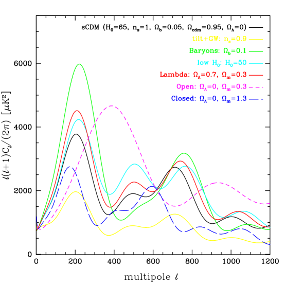
Figure 2: A sample of theoretical power spectra for various cosmological parameters, as marked.

The evolution of a single wavelength of perturbation is determined by a second order differential equation and thus has two independent solutions. When the Hubble length is smaller than the perturbation wavelength (which is the case at very early times, from soon after the perturbations creation in the inflationary epoch) only one of these independent solutions does not decay with time. Thus all perturbations are “squeezed” into the same state. A result is that all acoustic oscillations of a given wavelength all have the same temporal phase. This coherence is important to achieving the multiple peak structures seen in Figure 2.

The matter transport caused by the pressure and gravitational potential gradients means there are velocity perturbations as well. Hence, the photons can scatter off of moving electrons, which generates a net linear polarization of the photons polprimer . For the sound waves we are considering, the velocities are greatest when the density contrast is smallest, and vice versa: the velocity is out of phase with the density–and hence the polarization signal is out of phase with the temperature. Unfortunately, due to the relative inefficiency of scattering off of the moving electrons, the polarization fraction is only about 10%, and the polarization spectra are correspondingly suppressed.

We discuss polarization induced by gravitational waves in subsection VI.2.

V Current Status of CMB Measurements

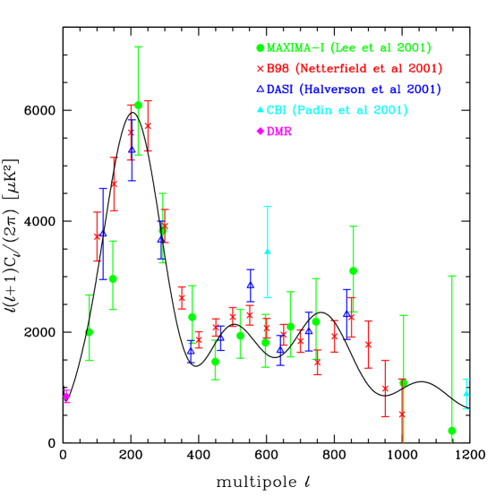
Figure 3: Recent measurements of the CMB power spectrum, from the experiments as listed and cited in the text. The smooth curve is a model chosen to fit an older subset of the data maxiboom01 , but remains a good fit to the current data.

In a real experimental setup, we measure the temperature (or intensity) of radiation, and its polarization in various directions. Traditionally, we measure components called $Q$ and $U$ giving two components $45^{\circ}$ apart (there is also another polarization component, $V$ which is zero in cosmological situations). Thus, we start with noisy measurements of $T$, $Q$ and $U$ on the sky, smeared by the instrumental beam. If we can extract the underlying signal, we can then relate these measurements to the power spectra predicted by theory. First, consider the temperature signal. We start with the temperature pattern on the sky, $\Delta T({\bf\hat{x}})/T=[T({\bf\hat{x}})-{\bar{T}}]/{\bar{T}}$, where ${\bar{T}}$ is the average temperature and ${\bf\hat{x}}$ is a unit vector, and expand this in spherical harmonic multipoles:

$$\frac{\Delta T}{T}({\bf\hat{x}})=\sum_{\ell m}a^{T}_{\ell m}Y_{\ell m}({\bf\hat{x}})$$ (4)

Under the assumptions of Gaussianity and an isotropic distribution on the sky, we can treat the components $a^{T}_{\ell m}$ as if they were drawn from a multivariate (but uncorrelated) Gaussian distribution with variance

$$\langle a^{T}_{\ell m}a^{T}_{\ell^{\prime}m^{\prime}}\rangle=C_{\ell}\delta_{\ell,\ell^{\prime}}\delta_{m,-m^{\prime}}\;.$$ (5)

Then, our task will be to determine $C_{\ell}$ from an actual noisy realization of some part of the sky. In the class of inflationary theories, these $C_{\ell}$ completely determine the statistics of the temperature pattern, and are completely determined by the cosmological parameters.

For polarization measurements, things are somewhat more complicated: we must first relate the $Q$ and $U$ measurements to the “gradient” and “curl” fields on the sky ($a_{\ell m}^{G}$ and $a_{\ell m}^{C}$, using so-called “tensor spherical harmonics” in place of the scalar $Y_{\ell m}$ of Eq. 5) (which can only be done statistically in the realistic case of noise, finite sky, and finite beam resolution), and in turn relate these to the various power spectra:

$$C_{\ell}^{XX^{\prime}}=\langle a_{\ell m}^{X}a_{\ell m}^{X^{\prime}}\rangle,$$ (6)

where $X,X^{\prime}=T,G,C$. From parity considerations it can be shown that only $C_{\ell}\equiv C_{\ell}^{TT}$, $C_{\ell}^{TG}$, $C_{\ell}^{GG}$ and $C_{\ell}^{CC}$ are nonzero (except in the presence of parity-violating physics). (All of this is a review of material first presented in  KamKosSte ; ZalSel97 )

V.1 Temperature and Polarization Power Spectrum Constraints

In Figure 3, we show a selection of recent measurements of the CMB temperature power spectrum, $C_{\ell}\equiv C_{\ell}^{TT}$. At the lowest $\ell$ (corresponding to the largest angular scales) we show a single point representing the measurement from the DMR instrument on the COBE satellite cobe . Over $50<\ell<1300$ we show points from four recent experiments with angular resolution of better than 20 arcmin. MAXIMA Lee01 and BOOMERANG netterfield01 are balloon-borne experiments using bolometers to measure the intensity of radiation; CBI CBI and DASI halverson00 ; pryke01 are ground-based interferometers. The recently-launched MAP satellite MAP promises to surpass these measurements over most of this regime. MAP will span the frequency range 30-90 GHz with an angular resolution of about $10^{\prime}$ at 90 GHz. The Planck Surveyor satellite Planck is due to be launched in 2007 and will give sample-variance-limited measurements of the temperature power spectrum out to $\ell\sim 1500$ where the information content becomes negligible due to damping effects. Planck covers a frequency regime of 30-850 GHz, with an angular resolution of $5^{\prime}$ at the highest frequencies.

In contrast, we are only now reaching the requisite sensitivity to detect polarization; upper limits on the polarization power spectrum are shown in Figure 4; they are now within an order of magnitude of the predicted RMS polarization.

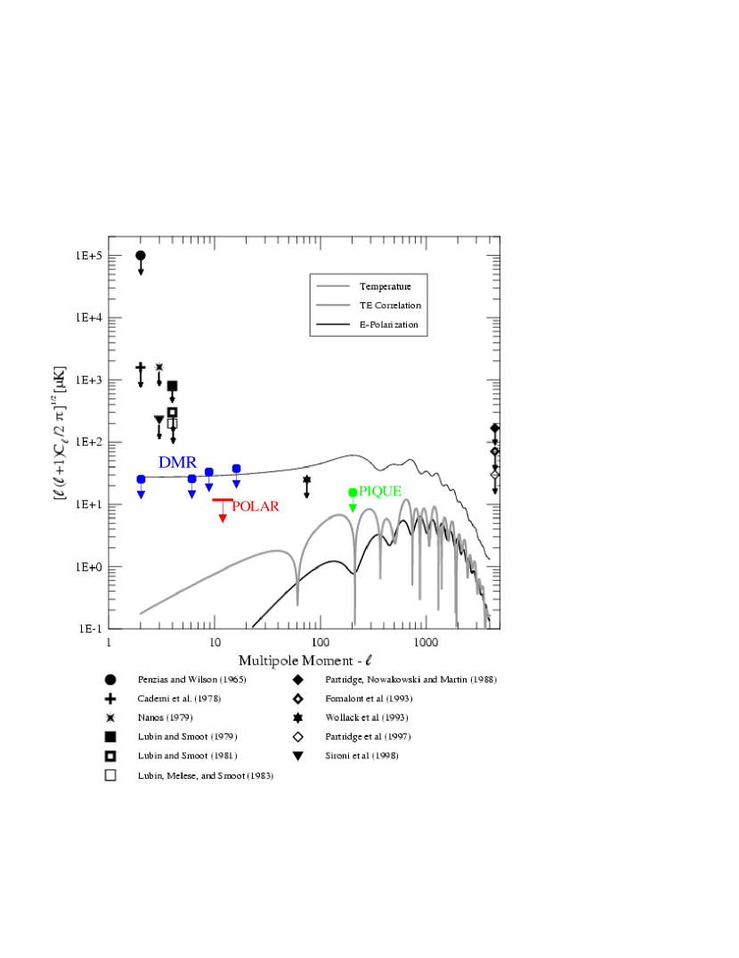
Figure 4: Current limits on the polarization of the CMB. From Ref. StaggsGundrvw , except for more recent points from POLAR POLAR01 , PIQUE PIQUE01 and unpublished limits from DMR DMRpol .

Although measurements of the CMB are providing remarkable quantitative constraints on cosmological parameters, we begin by emphasizing the following qualitative interpretations of the data:

• the initial perturbations were adiabatic with a nearly scale–invariant power spectrum,

• the mean spatial curvature is near zero,

• the acoustic oscillations are highly coherent.

These are all predictions of inflation. Whether they are unique to inflation is a matter of debate. Scale–invariant perturbations can be created without inflation and flat Universes are perhaps preferred by quantum–tunneling events. The theoretical prejudice for these two items actually precedes the first papers on inflation. It is the third item, the coherence of the acoustic oscillations, which makes the strongest case we have for an alteration of the causal structure of the space–time in some early epoch, as discussed in coherence1 .

In brief, the coherence can result from a ”non–dynamical” stage of perturbation evolution—when the wavelength of a given perturbation is larger than the Hubble radius. Thus the challenge is to create perturbations which are, for some period of time, larger than the Hubble radius. One cannot do this causally in a classical big–bang model without a period of inflation. This statement is almost definitional, since inflation is an acceleration of the scale factor and acceleration of the scale factor is what is required for the Hubble radius to grow more slowly than the scale factor. Causal analyses become more complicated in a brane–world picture, and there are scenarios in which super–Hubble radius perturbations are created without any acceleration of the scale factor ekpyrotic .

Quantitative cosmological constraints from current CMB measurements are also of great interest. As mentioned earlier what these constraints assume from inflation is an initially power–law power spectrum of adiabatic fluctuations. One of the best–measured parameters from CMB experiments is $\Omega_{\rm tot}$, which is equal to unity when the mean spatial curvature is zero. The results from the experiments are quite clear. From DASI, Boomerang and Maxima, $\Omega_{\rm tot}=1.01\pm.08,0.97\pm.10,1.0\pm.14$ respectively. Combining all these experiments and others wang01 results in $\Omega_{\rm tot}=1.0^{+.06}_{-.05}$. These results are significant for inflation since a non–zero curvature would make inflation a much less attractive early Universe scenario.

The power–law spectral index for the initial power spectrum of scalar perturbations, $n_{s}$, is also well–determined from the data. Once again from DASI, Boomerang and Maxima we have $n_{s}=1.04\pm.06,1.02\pm.06,1.08\pm.10$ respectively. The value $n_{s}=1$ is scale–invariant since for that value the contribution to the density variance from each decade of wavenumber is constant. Inflationary models produce values of $n_{s}$ in the range 0.8-1.2. Refined determinations of $n_{s}$ will thus not by themselves test inflation, but will rule out particular classes of inflationary models.

The stronger one’s model assumptions, the stronger the conclusions one can draw from CMB data. An interesting assumption, motivated by simplicity and the success of inflationary models, is the assumption that $\Omega_{\rm tot}=1$. With the mean curvature thus fixed, one can then use the peak locations (combined with assumptions about the Hubble constant) to determine $\Omega_{\Lambda}$ kamionkowski00 ; knox00 (or more generally some combination of the dark energy density and equation-of-state parameter, $w$). For example, if $h>0.55$ knox01 report $\Omega_{\Lambda}>0.4$ at 95% confidence. This gives an argument for the existence of dark energy which is independent of supernovae and constraints on the dark matter density.

Of course, the weaker one’s model assumptions the less one can say, and this model–dependence is important to keep in mind. The model space can be expanded in several ways. Allowing for tensor perturbations opens up $n_{s}$ to be in the“$2\sigma$” range 0.89-1.49 according to efstathiou01 and similar result in wang01 . As a more extreme example, allowing for arbitrary admixtures of various isocurvature modes together with the adiabatic mode makes most parameter constraints from the CMB large enough to be useless trotta01 .

The model–dependence of the CMB parameter constraints underscores the importance of other cosmological measurements such as galaxy redshift surveys, quasar spectrum studies of the Lyman-$\alpha$ forest and supernovae observations. These observations can either serve to support the modeling assumptions or further tighten parameter uncertainties. For example, adding in galaxy redshift survey information and BBN constraints on the baryon density shrinks the $n_{s}$ range cited above efstathiou01 by a factor of 3.

For probing inflation, we want the best information we can get on the primordial power spectrum, $P(k)$. In particular, it would be very helpful to see some departure from an exact power–law. To see any break we want to have as long a lever arm as possible and thus we want to complement CMB measurements with determinations of $P(k)$ on small scales. The best way to do this, at the moment, is with Lyman–$\alpha$ forest observations.  croft00 For the first attempts see Refs. hannestad01 ; zaldarriaga01 .

VI Motivation for Further Measurements

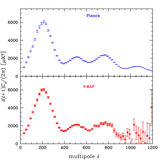
Figure 5: Projected error bars for the power spectrum from Map (bottom) and Planck (Top). We have binned the spectra with a width $\delta\ell=20$.

Two satellite missions that will greatly improve upon current measurements of the CMB are MAP and the Planck Surveyor. Simulated power–spectrum determinations for these missions are shown in Figure 5. As has been detailed elsewhere, these measurements will enable us to determine cosmological parameters to unprecedented precision forecast , to reconstruct the primordial density perturbation spectrum, $P(k)$ wang99 , and discriminate among inflationary models (see Figure 1).

Here we provide motivation for measurements with even higher sensitivity than those to be made by MAP and Planck. This higher sensitivity is necessary for measuring the polarization of the CMB and determining higher–order temperature correlations. For a review of future experiments designed to measure the temperature and polarization of the CMB, see the proceedings of working group E6.1 in this volume scgkt01 .

VI.1 Temperature

The Planck Surveyor, if it performs to specifications, will be practically the final word on the study of primary CMB temperature anisotropy. For $l\mathrel{\mathchoice{\lower 3.6pt\vbox{\halign{$\mathsurround=0pt\displaystyle\hfil#\hfil$\cr<\crcr\sim\crcr}}}{\lower 3.6pt\vbox{\halign{$\mathsurround=0pt\textstyle\hfil#\hfil$\cr<\crcr\sim\crcr}}}{\lower 3.6pt\vbox{\halign{$\mathsurround=0pt\scriptstyle\hfil#\hfil$\cr<\crcr\sim\crcr}}}{\lower 3.6pt\vbox{\halign{$\mathsurround=0pt\scriptscriptstyle\hfil#\hfil$\cr<\crcr\sim\crcr}}}}1500$, all the $C_{l}$’s will be determined to nearly the sampling variance limit; i.e., further reduction in the measurement noise will not reduce the $C_{l}$ uncertainty.

Further refinement of our knowledge of CMB temperature anisotropies is nevertheless well–motivated. With higher angular resolution and higher sensitivity maps one can study secondary effects in the CMB anisotropy, created much more recently than last–scattering. These secondary effects are created both gravitationally (via lensing and the “Integrated Sachs–Wolfe” (ISW) effect) and by Thomson scattering off of electrons in the post–reionization inter–galactic medium. Of particular interest for this report are the lensing and ISW effects because these can be used to break the degeneracy between $\Omega_{\Lambda}$ and $w$ which exists in constraints from the primary CMB data alone.

Hu hu01 considers complementing Planck with a CMB survey (called the “D” survey) covering one tenth of the sky with 1’ resolution (fwhm) and 10 $\mu$K per pixel errors. Such a map would be a probe of gravitational lensing and ISW effects in the CMB. The correlations between these two effects contribute to the three–point correlation function and depend on the amount of dark energy and its equation–of–state. Forecasted constraints on $\Omega_{\Lambda}$ and $w$ from MAP and Planck, complemented by the D survey, are shown in the top left panel of Fig. 6. Unfortunately, the constraints on $w$ are not very strong.

Since the lensing and ISW are late–time effects, associated with the more–local Universe, there is great value to be had from cross–correlating with other observables. Of particular value are galaxy lensinging surveys with source galaxies broken up into coarse redshift bands (Z). Indeed, the impact of such a survey in the $\Omega_{\Lambda}$–$w$ plane is much greater than for the D survey, as one can see in the lower panels of Fig. 6. Combining Planck with a 1000 sq. deg. Z survey leads to an error on $w$ of .05. Adding the D survey to Planck and Z reduces the error to 0.03. See hu01 for details. Also see verde01b .

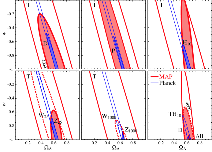
Figure 6: Improvement on the MAP (thick) and Planck (thin) temperature ($T$) determination of the dark energy equation of state and density. Clockwise from the top left: addition of CMB deflection angles ($D$); polarization ($P$); 10% Hubble constant measurements ($H$); 25 deg² cosmic shear survey with ($Z$ solid) and without ($W$ dashed) tomography; same but for 1000 deg²; Hubble constant ($TH$), plus deflections ($D$), plus a 1000 deg² lensing survey (All) (from hu01 ).

Astrophysical foregrounds have proven to be fairly benign for measurement of the CMB temperature $C_{l}$ over the important range of $l$ for primary CMB anisotropy. Whether this happy situation will extend to higher angular scales and to the higher sensitivity required for studying non–Gaussian properties of secondary anisotropies is not yet clear. Studying the non–Gaussian properties of available foreground maps would be a good first step towards incorporating these concerns into error forecasting.

VI.2 Polarization

In section  IV we considered polarization due to electrons moving with the fluid as it responds to the pressure and gravitational potential gradients. The polarization pattern that results is “curl-free”; that is, it can be represented as the 2-d divergence (gradient) of some scalar on the sky. This is easy to understand if we heuristically identify the polarization pattern with the flow of the plasma. In linear perturbation theory this flow is a potential flow; any vorticity is damped by expansion and not driven to grow by gravity.

Gravitational waves at last–scattering can produce a “curl” pattern, since gravity waves can produce non–potential flows in the plasma. For full-sky maps with high sensitivity and resolution, the “gradient” and “curl” components (also known as “Electric” and “Magnetic” or $E$ and $B$ from the obvious analogy to electromagnetic fields) can be separated completely; in more realistic situations statistical techniques are necessary.

Unfortunately, gravitational waves from inflation are not the only way to create polarization patterns with non–zero curl. Astrophysical foregrounds, such as emission from dust in our own galaxy and extragalactic point sources, will also produce some curl. These can be subtracted to some degree with the aid of multi–frequency measurements since they are spectrally distinct. Since their spectra aren’t perfectly known, however, there will always be some residual uncertainty in the subtraction. More insidious is the production of a curl pattern by non–linear evolution. Specifically, the deflection of light rays through latter-day large-scale structures will generate a curl patternhu01 ; ZalSel98 ; LewChaTur01b . This contribution can also be distinguished from the gravitational wave contribution via the shape of its power spectrum. However, the uncertainty in this subtraction will put a fundamental limit on the sensitivity of any polarization measurement to gravitational waves. This limit has not yet been calculated exactly but it’s approximately $r=10^{-3}$ LewChaTur01b where $r$ is the ratio of gravitational wave to density perturbation contributions to the temperature quadrupole variance, $C_{2}$. Translated into an energy scale of inflation, if this energy scale is below about $V^{1/4}=5\times 10^{15}$ GeV then $r<10^{-3}$ and we will never detect the influence of the gravity waves.

Detection of a curl pattern with the right photon spectrum and power spectrum would be very interesting. The amplitude of this pattern is proportional to the energy–scale of inflation. There is no other way of getting this information. And it would be more evidence of inflation as the generator of perturbations. Possibly this evidence would constitute a “smoking gun” but there is no proof of inflation’s uniqueness in this regard. Interestingly, one possible alternative for the generator of density perturbations, the ‘ekpyrotic Universe’, produces a gravity-wave background with a very small amplitude and bluer spectrum ekpyrotic . Other mechanisms for producing gravity waves (such as first order phase transitions) result in redder power spectra.

Whereas the Planck Surveyor will recover the entire primary temperature anisotropy, neither Planck nor any other currently planned and funded missions will achieve the same for polarization. Only a small fraction of the “E-mode” multipole moments from 2 to 2000 will be measured with signal–to–noise ratios greater than one. For the “B-mode,” if it comes from inflationary gravity waves, the situation is even less certain, since the overall amplitude of the signal depends on the energy scale of Inflation.

As our knowledge of CMB polarization increases — which it should do very rapidly over the next very few years, as we first detect it (expected in 2001-2002) and then measure the polarization spectra with some precision, we will begin to get a handle on the orders of magnitude of the instrumental and astrophysical problems. With this knowledge, we will be able to consider a more community-wide effort to measure polarization with the sensitivity necessary for an exploration of the B-mode signal (if present, of course). The time is ripe today to continue development of appropriate high-sensitivity technologies. What is needed is either radically new technologies for individual detectors or increasing the number of detectors from the $\sim 100$ aboard Planck by more than an order of magnitude. Whether such an instruments needs to be in space is still unclear and will depend in part on the magnitude of the foreground problem, and thus on the range of frequencies we will be required to cover in order to cleanly extract the cosmological signal. For more details on the hardware aspects of this problem, see the companion report of section E6.

VII Analysis Challenges

As the amount of CMB data has increased over the last decade, our understanding of the optimal analysis techniques has progressed alongside (for a fuller description, see, e.g., BCJK99 ). The analysis pipeline can be seen as several subsequent steps of data compressionBJK00 : from the raw data taken by the instrument, to a cleaned and calibrated timestream of data; from the timestream to a map on the sky (or, in the case of interferometers, to a set of visibilities); from the map (or visibilities) to the CMB power spectrum; and finally from the power spectrum to the cosmological parameters.

In the standard analyis techniques used today, we perform each of this steps using a Bayesian or maximum-likelihood formalism, usually under the assumption that the distributions of both the instrumental noise and the underlying cosmological signal can be treated as multivariate Gaussians, with covariance matrices given, respectively, by the instrumental noise characteristics (which must themselves be determined from the dataFerJafMNRAS00 ; Dore01 ), and the CMB power spectrum. This in turn means that the likelihood calculations require the manipulation of these matrices. Unfortunately, the manipulations required, at least for the brute-force solution to the likelihood equations, scale as the cube of the number of pixels. For data sets of even moderate size ($\sim 10,000$ pixels) this becomes prohibitive on an individual workstation (circa 2001); BorrillMADCAP has written the MADCAP package to perform the mapmaking and spectrum-estimation steps using standard libraries available on parallel supercomputers.

We note that the vast majority of analysis time is still spent understanding the systematic problems of any individual experiment (and even different incarnations of the same experiment); for examples of the work required, seestompor01Maps ; netterfield01 .

These quantitatively and qualitatively new data will bring with them new problems in their analysis. The first and most obvious is simply the amount of data. As stated above, the brute-force solution to the likelihood problem scales as the cube of the number of pixels. For the megapixel datasets of MAP and Planck, this will likely be impossible even with expected increases in processing power over the required timespan. Several new methods and ideas have already been explored. Here, we will discuss recent work in the most computationally-intensive phase of the analysis, the determination of the power spectrum.

The first possibility takes note of the fact that one reason for the $N^{3}$ scaling is that the instrumental noise and the CMB fluctuations have very different natural bases: the CMB fluctuations are expressed most naturally as spherical harmonics, whereas the instrumental noise is expressed in the timestream, or, after the mapmaking manipulations, in the pixel basis. In OSH99 , the authors show, for the special case of the expected performance of the MAP satellite, the instrumental noise can also approximately be expressed in the spherical-harmonic bases, and this approximation used as the basis for iterative schemes for the required matrix manipulations.

Another possibility uses the folk wisdom that high-$\ell$ information can be gathered separately from different parts of the sky, without performing the full analysis, whereas low-$\ell$ information only requires a smoothed version of the full data. In DoreKnox01 , the authors use this as the basis of a hierarchical decomposition of the dataset, iterating toward an approximation to the likelihood by combining the results for maps at different resolution levels and areas of the sky.

Yet another possible solution abandons the Bayesian approach entirely and tries to find frequentist statistics as estimators for the power spectrumHivon01 . That is, we first select some “natural” estimator for the power spectrum, such as the square of the windowed Fourier components of the noisy map, which is then modified by appropriate multiplicative and additive filters, determined so that the estimator is suitably unbiased with appropriately small variance. Finally, there has been some work (used in netterfield01 ) using these frequentist statistics within the likelihood formalism, as approximations to the shape of the likelihood in the “Bayesian” sense (as functions of the $C_{l}$ for fixed data).

All of the discussion so far has been directed toward the analysis of temperature data; polarization data presents its own set of problems. The most obvious is simply size, yet again: instead of just the temperature at each pixel, we now have two additional numbers describing the polarization: to analyze a map of the same size by brute-force techniques will take $\sim 3^{3}=27$ times as long. Moreover, the very low signal-to-noise of the polarized data will require far greater attention to systematic problems (and foregrounds) than is currently required by temperature data; only with real data in hand will we be able to explore these problems in any detail.

VIII SZ Surveys

As discussed in Section V accurate measurements on the CMB will set tight constraints on the relative densities of baryonic matter, dark matter and dark energy at the surface of last scattering. In addition, one particular combination of these densities, the curvature, and the dark energy equation of state parameter, $w$, will be well–determined—that combination which fixes the ratio of angular–diameter distance to last-scattering surface to the sound horizon at last scattering.

However, as shown in Fig. 6, CMB measurements cannot, by themselves, separately determine the dark energy density and $w$. In particular, they are highly unlikely to distinguish a cosmological constant ($w=-1$) from any of the currently viable alternatives. For example, the dark energy may be the result of a slowly evolving scalar field, with $w>-1$ and time–varying ws98 ; wco99 .

Measurements of large scale structure offer good prospects for probing $w$. Dark energy manifests itself as a smooth component that will inhibit the gravitational collapse of structure once the dark energy density begins to exceed the density of gravitating matter. The value of $w$ also affects the comoving volume in solid angle $d\Omega$ from redshift $z$ to redshift $z+dz$, and therefore how comoving densities are translated into observables.

Galaxy clusters are the largest virialized objects in the universe and are believed to have formed relatively late (at $z=1$–3). Clusters are important cosmological probes for several reasons. First they represent the accumulation of matter from quite large regions of the universe and so one may assume that their contents are representative of the universe as a whole. Most of the baryonic matter in clusters is contained in hot gas trapped in the cluster potential well which can be detected via the Sunyaev-Zel’dovich effect (see below) or from X-ray measurements of bremsstrahlung emission. The total mass of the cluster can be deduced from weak gravitational lensing if such data are available, or from the spatial distribution of the gas, with an assumption that the gas is in hydrostatic equilibrium. In this way clusters can be used to constrain $\Omega_{b}/\Omega_{m}$ 2001ApJ…552….2G where $\Omega_{b}$ and $\Omega_{m}$ are the density parameters of baryonic matter and all matter, respectively. Second, the details of cluster formation can be modeled in a straightforward way since they depend primarily on the details of the gravitational collapse of structure, and not on more “messy” processes such as gas dynamics and energy injection from star formation (although see Section VIII.4.1). As a result, the masses of clusters and their distribution in redshift is primarily sensitive to purely cosmological factors such as:

• The initial power spectrum of matter fluctuations, characterized by $\sigma_{8}$, the rms fluctuation in mass in a region with radius 8$h^{-1}$ Mpc, and $n$, the spectral index of density fluctuations on the scale of clusters.

• The rate of growth of structure via gravitational collapse.

• The geometry of the universe, since this determines the size of a volume element at a given redshift.

As discussed below, the Sunyaev-Zel’dovich effect offers excellent prospects for using galaxy clusters in this way.

VIII.1 The Sunyaev-Zel’dovich Effect

The Sunyaev Zel’dovich (SZ) effect sz72 is the result of the interaction of the CMB with ionized gas along a line-of-sight to the surface of last-scattering. Compton-scattering of CMB photons by the much hotter electrons in the gas causes a distortion, $\Delta I_{\rm th}$ to the intensity, $I_{\rm CMB}$, which in the non-relativistic limit is given by:

$$\frac{\Delta I_{\rm th}}{I_{\rm CMB}}=\frac{xe^{x}}{(e^{x}-1)}\left[x\coth\frac{x}{2}-4\right]\times y_{\rm th}\mbox{\hskip 14.22636pt where \hskip 14.22636pt }y_{\rm th}=\sigma_{T}\int n_{e}\frac{kT_{\rm e}}{m_{\rm e}c^{2}}{\rm d}l$$ (7)

with $x=h\nu/kT_{\rm CMB}$. The quantity $y_{\rm th}$ is proportional to the pressure of the gas integrated along the line-of-sight to the last scattering surface and depends on $T_{\rm e}$, the temperature of the gas, $\sigma_{T}$, the Thompson cross-section, and $n_{e}$, the electron density. The hottest gas is located in cluster potential wells and can be as hot as 15 keV, and consequently clusters will dominate the SZ signal. However, the CMB acts as a uniform back-light to all of the hot gas in the universe, including the cooler, less-dense gas with temperature 8–800 eV which is predicted from simulations of large scale structure formation to exist as a filamentary structure between clusters. cen99

The distortion characterized by $y_{\rm th}$ is known as the thermal SZ effect because the amplitude is related to the thermal motions of the electrons in the clusters. The thermal SZ effect has a unique spectral shape (see Fig. 7) causing a rich cluster to appear as a “hole” in the CMB at low frequencies, but as an increase in the CMB intensity at frequencies above $\sim 217$ GHz. Eq. 7 is valid only in the non-relativistic limit, so for most rich clusters, corrections to the spectrum at the level of a few percent are necessary nsi00 ; reph95 . This causes the frequency of the null of the thermal effect, and the overall shape of the spectrum, to be weakly dependent on the gas temperature.

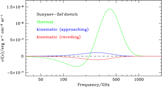
Figure 7: Brightness of the SZ effect as a function of frequency. The solid line is the thermal component (in the non-relativistic limit), the two dotted lines show the kinetic component. The sign of the kinetic component depends on the direction of the cluster peculiar velocity relative to the observer. The assumed parameters are $\tau=1$%, $T_{e}=5$ keV, and $v_{\rm pec}$=1000 km/s.

In addition to the thermal effect, there is a second component – the kinematic SZ effect – which is the result of the bulk motion of the plasma in the rest frame of the CMB. In the non-relativistic limit, the change in brightness is given by:

$$\frac{\Delta I_{\rm kin}}{I_{\rm CMB}}=\frac{xe^{x}}{(e^{x}-1)}\times y_{\rm kin}\mbox{\hskip 14.22636pt where \hskip 14.22636pt}y_{\rm kin}=\sigma_{T}\int n_{e}\frac{{\bf v}_{\rm pec}\cdot{\rm d}{\bf l}}{c}=\tau\frac{v_{\rm pec}}{c}$$ (8)

Here $v_{\rm pec}$ is the mean radial component of the peculiar velocity of the cluster plasma, ${\bf v}_{\rm pec}$. The optical depth, $\tau$, of a rich cluster is typically 1%. The spectral profile of the kinematic SZ effect is also shown in Figure 7. The kinematic effect has yet to be detected, but since cluster peculiar velocities are expected to be no more than a few hundred km/s 1994ApJ…430L..13B ; 1996MNRAS.282..384M the kinematic effect is likely to be at least an order of magnitude fainter than the thermal effect.

The expressions in Eqs. 7 and 8 allow the determination of the SZ effect along a given line of sight through a cluster, This quantity has no explicit redshift dependence because the effect is a scattering process and both $\Delta I$ and $I_{\rm CMB}$ scale in the same way with redshift. Consequently, the amplitude and spectral shape of the SZ effect are independent of the distance to the cluster. Of course, the redshift does affect the total SZ flux from a cluster. Assuming that a cluster is approximately isothermal, the integrated flux from a cluster at redshift $z$ is:

$$S=\frac{i_{0}0(\nu)}{d_{A}^{2}(z)}\times\frac{kT_{e}}{m_{e}c^{2}}\frac{\sigma_{T}f_{\rm ICM}}{\mu_{e}m_{p}}\times M_{v}$$ (9)

where:

$$i_{0}(\nu)=2kT_{\rm CMB}\left(\frac{kT_{\rm CMB}}{hc}\right)^{2}\frac{x^{4}e^{x}}{(e^{x}-1)^{2}}\left[x\coth\frac{x}{2}-4\right]$$ (10)

The quantity $d_{A}(z)$ is the angular diameter distance to the cluster, $M_{v}$ is the mass of the cluster contained in the virial radius, $\mu_{e}=1.15$ is the mean molecular weight per electron, $f_{\rm ICM}$ is the fraction of the mass contained in the intracluster medium (ICM) and $m_{p}$ is the proton mass. Various forms of Eq. 9 can be found in Refs. bbbo96 ; hc01 ; vhs01 .

From Eq. 9, it can be seen that although there is a dependence of total flux on redshift, it is much weaker than for other sources of emission such as X-ray flux which decreases by an extra factor of $1/(1+z)^{4}$ as the redshift increases. This makes the SZ effect a prime technique for detecting clusters of galaxies out to the epoch of cluster formation.

VIII.2 Prospects for SZ Measurements

For a comprehensive review of the current status and future prospects of SZ measurements, the reader is referred to the proceedings of E6.1 in this volume scgkt01 , and also to carl00 . The first detections of the SZ effect required many years of pioneering work 1990cmwb.book…77B but in the past 5 years, detections of the thermal SZ effect in rich clusters identified from X-ray surveys have become routine. SZ measurements have been used to obtain estimates of the Hubble constant, of the gas mass fraction in clusters and of the peculiar velocities of galaxy clusters. Fig. 8 shows the type of data that can now be routinely obtained with existing instruments.

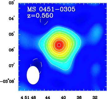
Figure 8: Left: Map of the SZ decrement towards the high redshift cluster MS0451 made using the BIMA array (from rmc00 , courtesy J. Carlstrom.). Right: Measurement of the spectrum of MS0451 using the flux measured with the BIMA array (cross) and the SuZIE experiment (stars) bc01 .

Figure 9: Current limits on the SZ power spectrum. CBI ; cb01 ; daw01 ; sub00 The solid line is the best-fit CMB power spectrum to the CBI point (generated with CMBFAST sel96 ). The two dashed lines are two models for the power spectrum of the thermal SZ effect that reflect different assumptions regarding the evolution of the cluster gas 1999mifo.conf..199H ; 2001ApJ…549..681S (see Section VIII.4.1).

Blind searches with existing SZ instruments for clusters not previously identified in optical or X-ray surveys have either been unsuccessful or have produced ambiguous results which have not been verified elsewhere. This is because existing instruments, although excellent for investigation of known clusters, lack the sensitivity and sky coverage required and the observations shown in Fig. 8 typically take many hours. Fig. 9, which shows current limits on the SZ power spectrum give an indication of the gap between the current and the ideal experiment. A new set of experiments has been proposed with emphasis on large areas of sky and multi-frequency observations to separate SZ from intrinsic CMB. These experiments are reviewed in detail in the E6.1 proceedings in this volume scgkt01 and can be divided into the following catagories:

• Deep surveys of about 10 sq deg. with radio interferometers should achieve a limiting mass of $10^{14}$ M_⊙ carl98 ; kjs01 and will obtain high resolution maps of individual clusters.

• Medium-deep surveys of about 100-4000 sq deg. using bolometer arrays on 6-m class telescopes expect to achieve a limiting mass of $2$–$4\times 10^{14}$ M_⊙ hhm01 ; vhs01 .

• Shallow Surveys The all-sky survey from the Planck Surveyor will achieve a mass limit of $8\times 10^{14}$ M_⊙ bbbo96

VIII.3 Science from the SZ Effect

Fig. 10, from hhm01 , simulates the limits that such SZ surveys will set on a variety of cosmological parameters (see also ws98 ; hmh01 ).

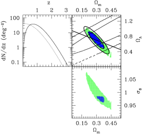
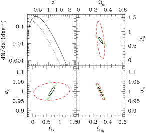
Figure 10: The ability of cluster surveys to probe cosmological parameters (figure from hhm01 , courtesy of G. Holder). The upper left panel of each figure shows the expected differential counts of clusters (the dashed line shows the cumulative numbers). The ellipses in the remaining panels show 68% and 95% confidence limits. The surveys are, from left to right, deep, medium deep and shallow, as defined in Section VIII.2.

VIII.3.1 Using the SZ effect to Probe Dark Energy

Because the number density of clusters is sensitive to the epoch at which cluster formation ends, this statistic constrains the allowable value of $w$. Fig. 11 shows the dependence of the number density of clusters with $M>10^{14}$ M_⊙ on $z$ for different values of $w$. The variation is caused by the dependence of the size of a volume element on $w$. The ability of cluster counts on the sky to constrain $w$ is explored more fully in hmh01 who show that the constraints are orthogonal to those provided by SNIa measurements. The number density depends on the integrated growth of structure, effectively integrating expansion from time zero to the present day. In contrast, SN 1a observations measure the angular diameter distance which is a function of integral of expansion from present day back to the cluster.

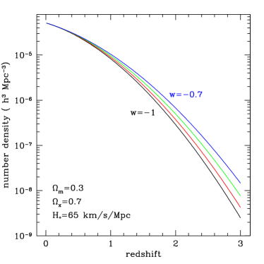
Figure 11: Number of clusters with $M>10^{14}$ M_⊙ as a function of redshift for different values of $w$ (figure courtesy of G. Holder)

The SZ effect can also be used in conjunction with X-ray measurements of a cluster to probe the dependence of angular diameter distance, $d_{A}$, on redshift. The X-ray surface brightness of a cluster is given by:

$$S_{x}=\frac{1}{4\pi(1+z)^{4}}\int n_{e}n_{H}\Lambda_{eH}{\rm d}l$$ (11)

where $n_{H}$ is the number density of hydrogen atoms in the ICM and $\Lambda_{eH}$ is the X-ray cooling function integrated over the observing band appropriate for the X-ray observation. By combining a measurement of $y_{\rm th}$, which depends on the integral of $n_{e}$ along a line of sight through the cluster, with measurements of the X-ray surface brightness, which depends on the integral of $n_{e}^{2}$ along the same line of sight, the linear depth of the cluster gas can be deduced. If the cluster is assumed to be spherically symmetric, then by comparing the measured depth with the angular extent of the cluster gas on the sky, the angular diameter distance to the cluster and thus $H_{0}$ can be determined. The accuracy from a single cluster is very low because of asphericity – clusters are not spherical as is assumed in the $d_{A}$ calculation. This can be corrected for by observing many clusters at the same redshift. Observations of 20-30 clusters, yields an estimate of $H_{0}=63\pm 3$ km s^-1 Mpc^-1 (assuming statistical errors only)  carl00 . A second source of uncertainty is clumping of the hot gas. If the clumping factor $C=<n_{e}^{2}>^{1/2}/<n_{e}>$, then the Hubble constant is overestimated by a factor $C^{2}$ carl00 . Consequently, a better understanding of the gas will be necessary to reliably determine angular diameter distances.

Assuming that clumping issues can be understood, a sample of at least 60 clusters kjs01 at a range of redshifts will determine $d_{A}(z)$ to a precision similar to that which has been obtained from SN1a measurements. Such samples are within reach of existing experiments and will be easily obtained by planned cluster surveys, with the caveat that X-ray and optical follow-up measurements must also be obtained (see Section VIII.4).

VIII.3.2 Other Cosmological Parameters from SZ Surveys

Using the SZ Effect to Probe Baryonic Matter Observations of the SZ effect complement other tracers of clusters physics such as weak gravitational lensing, and X-ray measurements. Like X-ray measurements, SZ measurements are sensitive to the amount of hot gas in the cluster. However, because the X-ray surface brightness is proportional to $\int n_{e}^{2}{\rm d}l$, the SZ effect is better able to trace cooler, low-density gas in the outskirts of a cluster, or between clusters. Consequently, the SZ effect is a important tracer of the distribution of baryonic matter in the universe.

Using the SZ Effect to Probe Dark Matter Separation of the two components of the SZ effect allows a direct measurement of $v_{\rm pec}$. For an isothermal plasma, the peculiar velocity can be derived from the SZ effect as follows:

$$\frac{v_{\rm pec}}{c}=\frac{y_{\rm kin}}{y_{\rm th}}\frac{kT_{\rm e}}{m_{\rm e}c^{2}}.$$

In principle, the gravitational potential that reflects the distribution of all matter, including non-baryonic dark matter, can be reconstructed from the peculiar velocity field, which comprises the residual motions of matter over and above the Hubble flow. Both the evolution of bulk flows with redshift and the amplitude distribution of peculiar velocities are also important observables that can be used to test cosmological models (see cd01 for a review). For distances greater than $\sim 150h^{-1}$ Mpc, uncertainties in distance measurements become too large to allow peculiar velocities to be determined accurately using traditional techiques which rely on distance determinations. The SZ effect provides us with a way to measure the peculiar velocity of clusters relative to the CMB with a precision that is redshift independent.

As is clear from Figure 7 however, the thermal and kinetic components can be separated only by measurements at mm wavelengths, close to the null of the thermal effect. In addition, the relatively small amplitude of the kinetic effect requires high sensitivity in order to measure the effect with precision. The ultimate limit to the peculiar velocity determination of a single cluster comes from intrinsic CMB anisotropies which have a spectrum that is indistinguishable from the kinematic SZ effect. The limits are expected to be about $200\times(0.01/\tau)$ km s^-1 for an experiment with a beam size of 1-2^′ 1996MNRAS.279..545H . However, this limit is independent of redshift, unlike empirical determinations of peculiar velocity. The Planck Surveyor, which will survey the whole sky at 22–850 GHz, will provide a peculiar velocity survey that can used to set limits of $50$–$200$ km s^-1 to the bulk flows of 100$h^{-1}$ Mpc volumes of space 1997A&A…325….9A ; 2001A&A…374….1A . Follow-up measurements using ground-based instruments with higher angular resolution will be able to set similar limits to smaller regions of space, although the experiment is likely to be very time consuming. Again, redshift information from optical follow-up is needed to fully exploit peculiar velocity measurements.

VIII.4 Outstanding Issues

VIII.4.1 Limits of modeling

The use of cluster number counts to constrain cosmological parameters assumes that the physics of cluster formation is understood. As discussed above, the simplest model of cluster formation assumes that clusters are virialized objects whose collapse is described by gravitational collapse alone, and the predictions of results from SZ surveys discussed here are based on that assumption. In practice other mechanisms such as feedback from galaxy formation, or mergers can modify the results, especially for low-mass clusters vhs01 ; hc01 . Simulations are becoming quite sophisticated but there is still substantial disagreement between different results, as shown in Fig. 10 which shows a range of predictions for the SZ power spectrum. As the sophistication of numerical modeling improves, with the added constraint of multi-frequency investigations of known clusters, these uncertainties should reduce.

Figure 12: Simulations of the power spectrum of SZ thermal fluctuations by several authors, from 2001ApJ…549..681S (courtesy of M. White).

VIII.4.2 Follow-up of Large Cluster Samples

Future SZ surveys will provide a large cluster sample for which the SZ flux, $y_{\rm th}$, and possibly $y_{\rm kin}$, will be determined. In order to fully exploit the science from this sample, a well-planned program of follow-up observations will be needed. The most critical component will be optical follow-up to determine cluster redshifts. This will be a time-consuming task requiring large amounts of time on large telescopes. In addition, X-ray measurements will be needed for programs to determine $d_{A}(z)$ and peculiar velocities.

- (1) A. Linde, Physics Reports333, 575 (2000).
- (2) A. H. Guth, Physics Reports333, 555 (2000).
- (3) V. Mukhanov, H. Feldman, and R. Brandenberger, Physics Reports215, 203 (1992).
- (4) D. Cormier and R. Holman, Phys. Rev. D60, 1301+ (1999).
- (5) S. Dodelson, W. H. Kinney, and E. W. Kolb, Phys. Rev. D56, 3207 (1997).
- (6) E. W. Kolb and M. S. Turner, The Early Universe (Frontiers in Physics, Addison-Wesley, Reading, MA, 1990).
- (7) P. J. E. Peebles, Principles of physical cosmology (Princeton Series in Physics, Princeton University Press, Princeton, NJ, 1993).
- (8) W. Hu, D. Scott, and J. Silk, Phys. Rev. D49, 648 (1994).
- (9) U. Seljak and M. Zaldarriaga, ApJ469, 437 (1996).
- (10) A. Lewis, A. Challinor, and A. Lasenby, ApJ538, 473 (2000).
- (11) W. Hu and M. White, New Astronomy 2, 323 (1997).
- (12) A. H. Jaffe et al., Physical Review Letters 86, 3475 (2001).
- (13) M. Kamionkowski, A. Kosowsky, and A. Stebbins, Phys. Rev. D55, 7368 (1997).
- (14) M. Zaldarriaga and U. Seljak, Phys. Rev. D55, 1830 (1997).
- (15) http://space.gsfc.nasa.gov/astro/cobe/.
- (16) A. T. Lee et al., (2001), astro-ph/0104459.
- (17) C. B. Netterfield et al., (2001), astro-ph/0104460.
- (18) S. Padin et al., Astrophys. J. Lett.549, L1 (2001).
- (19) N. W. Halverson et al., (2001), astro-ph/0104489.
- (20) C. Pryke et al., (2001), astro-ph/0104490.
- (21) http://map.gsfc.nasa.gov/.
- (22) http://astro.estec.esa.nl/SA-general/Projects/Planck/.
- (23) S. Staggs, J. Gundersen, and S. Chruch, in Microwave Foregrounds, edited by A. de Oliveira-Costa and M. Tegmark (ASP, ADDRESS, 1999).
- (24) B. G. Keating et al., Astrophys. J. Lett.560, L1 (2001).
- (25) M. M. Hedman et al., Astrophys. J. Lett.548, L111 (2001).
- (26) G. Smoot (unpublished).
- (27) J. Magueijo, A. Albrecht, P. Ferreira, and D. Coulson, Phys. Rev. D54, 3727 (1996).
- (28) J. Khoury, B. A. Ovrut, P. J. Steinhardt, and N. Turok, (2001), hep-th/0103239.
- (29) X. Wang, M. Tegmark, and M. Zaldarriaga, (2001), astro-ph/0105091.
- (30) M. Kamionkowski and A. Buchalter, (2000), astro-ph/0001045.
- (31) L. Knox, in Particles, Strings and Cosmology (World Scientific, Singapore, 2000), p. 326.
- (32) L. Knox, N. Christensen, and C. Skordis, (2001), astro-ph/0109232.
- (33) G. Efstathiou et al., (2001), astro-ph/0109152.
- (34) R. Trotta, A. Riazuelo, and R. Durrer, (2001), astro-ph/0104017.
- (35) R. Croft et al., ApJ, submitted (2000), astro-ph/0012324.
- (36) S. Hannestad, S. Hansen, F. Villande, and A. Hamilton, (2001), astro-ph/0103047.
- (37) M. Zaldarriaga, L. Hui, and M. Tegmark, ApJ557, 519 (2001).
- (38) D. J. Eisenstein, W. Hu, and M. Tegmark, ApJ518, 2 (1999).
- (39) Y. Wang, D. N. Spergel, and M. A. Strauss, ApJ510, 20 (1999).
- (40) S. Staggs et al., to appear in report from Snowmass 2001: The Future of Particle Physics (2001).
- (41) W. Hu, (2001), astro-ph/0108090.
- (42) L. Verde and D. N. Spergel, (2001), astro-ph/0108179.
- (43) M. Zaldarriaga and U. . Seljak, Phys. Rev. D58, 3003 (1998).
- (44) A. Lewis, A. Challinor, and N. Turok, (2001), astro-ph/0108251.
- (45) J. R. Bond, R. G. Crittenden, A. H. Jaffe, and L. E. Knox, Computers in Science and Engineering 1, 21 (1999).
- (46) J. R. Bond, A. H. Jaffe, and L. Knox, ApJ533, 19 (2000).
- (47) P. G. Ferreira and A. H. Jaffe, Mon.Not.Roy.As.Soc.312, 89 (2000).
- (48) O. Doré et al., A&A374, 358 (2001).
- (49) http://www.nersc.gov/~borrill/cmb/madcap.html.
- (50) R. Stompor et al., (2001), astro-ph/0106451.
- (51) S. P. Oh, D. N. Spergel, and G. Hinshaw, ApJ510, 551 (1999).
- (52) O. Dore, L. Knox, and A. Peel, Phys. Rev. D64, 083001 (2001).
- (53) E. Hivon et al., (2001), astro-ph/0105302.
- (54) L. Wang and P. J. Steinhardt, ApJ508, 483 (1998).
- (55) L. Wang, R. R. Caldwell, J. P. Ostriker, and P. J. Steinhardt, ApJ530, 17 (2000).
- (56) L. Grego et al., ApJ552, 2 (2001).
- (57) R. Sunyaev and Y. B. Zel’dovich, Comments Ap. Space Phys. 4, 173 (1972).
- (58) R. Cen and J. Ostriker, ApJ514, 1 (1999).
- (59) S. Nozawa, N. Itoh, Y. Kawana, and Y. Kohyama, ApJ536, 31 (2000).
- (60) Y. Rephaeli, ApJ371, L1 (1995).
- (61) N. A. Bahcall, R. Cen, and M. Gramann, Astrophys. J. Lett.430, L13 (1994).
- (62) L. Moscardini et al., Mon.Not.Roy.As.Soc.282, 384 (1996).
- (63) D. Barbosa, J. G. Bartlett, A. Blanchard, and J. Oukbir, A&A 314, 13 (1996).
- (64) G. P. Holder and J. E. Carlstrom, ApJ558, 515 (2001).
- (65) L. Verde, Z. Haiman, and D. N. Spergel, ApJsubmitted (2001), astroph/0106315.
- (66) J. E. Carlstrom et al., in Constructing the Universe with Clusters of Galaxies, edited by F. Durret and D. Gerbal (IAP 2000 meeting, Paris, France, 2000).
- (67) M. Birkinshaw, in ASSL Vol. 164: The Cosmic Microwave Backround: 25 Years Later (Kluwer Academic Publishers, Dordrecht, Netherlands, 1990), pp. 77–94.
- (68) E. D. Reese et al., ApJ533, 38 (2000).
- (69) B. Benson et al. (unpublished).
- (70) S. Church et al. (unpublished).
- (71) K. S. Dawson et al., Astrophys. J. Lett.553, L1 (2001).
- (72) R. Subrahmanyan et al., Mon.Not.Roy.As.Soc.315, 808 (2000).
- (73) U. Seljak and M. Zaldarriaga, ApJ469, 437 (1996).
- (74) G. P. Holder and J. E. Carlstrom, in ASP Conf. Ser. 181: Microwave Foregrounds (ASP, San Francisco, 1999), pp. 199+.
- (75) V. Springel, M. White, and L. Hernquist, ApJ549, 681 (2001).
- (76) J. Carlstrom et al., Physica Scripta, volume T 85, 148 (2000).
- (77) R. Kneissl et al., Mon.Not.Roy.As.Soc.(2001), astro-ph/0103042.
- (78) G. Holder, Z. Haiman, and J. J. Mohr, ApJ560, L111 (2001).
- (79) Z. Haiman, J. J. Mohr, and G. P. Holder, Ap. J. 553, 545 (2001).
- (80) S. Courteau and A. Dekel, in Astrophysical Ages and Time Scales (ASP Conference Series, San Francisco, 2001), p. in press.
- (81) M. G. Haehnelt and M. Tegmark, Mon.Not.Roy.As.Soc.279, 545 (1996).
- (82) N. Aghanim et al., A&A325, 9 (1997).
- (83) N. Aghanim, K. M. Górski, and J.-L. Puget, A&A374, 1 (2001).