THE GRAVITATIONAL LENS B1608+656:
I. V, I, AND H-BAND HST IMAGING
Abstract
We present a multi-wavelength analysis of high-resolution observations of the quadruple lens B1608+656 from the HST archive, acquired with WFPC2 through filters F606W (V-band) and F814W (I-band), and with NIC1 in filter F160W (H-band).
In the three bands, the observations show extended emission from the four images of the source in a ring-like configuration that surrounds the two, resolved, lensing galaxies. B1608+656 was discovered as a double-lobed radio source, and later identified as a post-starburst galaxy in the optical. Based on photometry and optical spectroscopy we estimate that the stellar population of the source has an age of 500 Myr. This provides a model for the spectrum of the source that extends over spectral regions where no observations are available, and is used to generate Tiny Tim PSFs for the filters. Deconvolutions performed with the Lucy-Richardson method are presented, and the limitations of these restorations is discussed. VI and IH color maps show evidence of extinction by dust associated with one of the lensing galaxies, a late type galaxy presumably disrupted after its close encounter with the other lens, an elliptical galaxy. The extinction affects the two lens galaxies and two of the four multiple images. The diagnostic of wavelength-dependent effects in the images shows that corrections for contamination with light from the lenses, extinction, and PSF convolution need to be applied before using the extended structure in the images as a constraint on lens models. We will present the restoration of the images in a subsequent paper.
1 INTRODUCTION
The discovery of the first gravitational lens was announced by Walsh, Carswell & Weymann (1979), long after a number of theoretical papers on lensing had appeared in the 1930s and 1960s. Since then several consequences of the lensing effect, including strong lensing, weak lensing, and microlensing, have been observed. In a strong lensing situation, a gravitational deflector lying close to the line of sight to a background source creates multiple images of the source. Strong lenses provide a powerful tool to study the distribution of matter, including the dark matter, in the lensing galaxies, and to measure the Hubble constant from the time delay between the multiple images (Refsdal, 1964). One of the most promising candidates for this analysis is the quadruple lens B1608+656, due to the quality of the observations.
The lens B1608+656 was discovered using the Very Large Array during a directed search for radio lenses by the Cosmic Lens All-Sky Survey (CLASS) (Myers et al., 1995); two months later it was rediscovered in another independent survey aimed at studying faint peaked radio sources (Snellen et al., 1995). The source was found to consist of four flat-spectrum components arranged in a typical “quad” configuration, with a maximum separation of 2.1” between components. Follow-up optical and infrared observations showed a similar morphology and revealed the lensing galaxy, confirming the lens hypothesis (Myers et al., 1995; Fassnacht et al., 1996). Optical spectroscopy with the Palomar 5 m telescope measured a redshift of zl=0.6304 for the lensing galaxy (Myers et al., 1995), and gave a redshift of zs=1.394 for the source, which was also identified as a post-starburst or E+A galaxy (Fassnacht et al., 1996). Monitoring of the radio variability of the source allowed the measurement of the three independent time delays between the components (Fassnacht et al., 1999).
Several models reproducing the image positions, relative fluxes and relative time delays in B1608+656 have already been constructed (Myers et al., 1995; Blandford & Kundić, 1996; Koopmans & Fassnacht, 1999; Surpi & Blandford, 2001). One conclusion obtained from these attempts is that modeling of the point source properties is under-constrained and several solutions are possible (Surpi & Blandford, 2001). Additional constraints, from the extended emission of the source, need to be incorporated to break this degeneracy and allow for an accurate lens model and determination of the Hubble constant from the measured time delays.
High resolution optical and near infrared imaging of B1608+656 with the Hubble Space Telescope (HST) has been acquired through four different filters. In this paper we present an analysis of the V, I, and H-band archive exposures of B1608+656 from HST proposals 6555 and 7422. This set offers a good multi-wavelength image sample of B1608+656 in terms of signal-to-noise. The high resolution obtained in the three bands reveals the extended structure of B1608+656. We compare the images and present a diagnostic of wavelength-dependent distortions in the surface brightness of the source, that are superposed on the distortions generated by the gravitational lens deflections. Once identified, the chromatic effects need to be corrected before using the extended emission of the source as a constraint on lens model. The reconstruction of the images is the subject of a coming paper (G. Surpi & R. Blandford, in preparation, hereafter Paper 2).
The organization of this paper is as follows. In §2 we discuss the B1608+656 observations, starting with a summary of the results from radio monitoring in §2.1, followed in §2.2 by a report of the optical and infrared exposures already taken with HST. §3 describes the process applied to combine the F606W, F814W and F160W exposures, and compares the V, I, and H band images obtained. In §4, we estimate the age of the post-starburst population in the source and adopt a model for its spectrum. In §5, we deconvolve the images using Tiny Tim generated point-spread-functions (PSF) and the Lucy-Richardson method for deconvolution. §6 describes VI and IH color maps and the evidence of extinction in the system. In §7, we discuss the properties of the optical and infrared images of B1608+656 and their potential use in the modeling of the lens mass distribution. Appendix A contains details on the processing of the V and I images, and Appendix B on the processing of H image.
2 OBSERVATIONS OF B1608+656
2.1 Radio Properties
The gravitational lens B1608+656 was discovered with the VLA at 8.4 and 15 GHz by two independent radio surveys in 1994 (Myers et al., 1995; Snellen et al., 1995). The radio images show the system consists of four well-separated components A, B, C, and D, all of them having flat radio spectra. The radio positions and flux densities of the components, as determined by recent VLA 8.4 GHz observations of the system (Fassnacht et al., 1999), are listed in Tab. 1. When a core of 51 mJy is subtracted at 1.4 GHz, the source is a radio galaxy with double-lobed structure having an overall size of 50” and an integrated flux density of 12 mJy (Snellen et al., 1995). The spectrum of the core is flat, while the double-lobe contribution can be modeled with a spectral index of (). One of the lobes is highly polarized, while the other one is unpolarized. The core exhibited variability by up to 15% at a frequency of 8.4 GHz, allowing for the possibility to determine the time delays in the system.
| Component | Position (”)aaPosition offsets with respect to component A in Cartesian coordinates, positive -axis points west (Fassnacht et al., 1999). | Flux Density (mJy)bbResults from the first season of VLA monitoring (Fassnacht et al., 1999). | Relative FluxbbResults from the first season of VLA monitoring (Fassnacht et al., 1999). | Time Delay (days)bbResults from the first season of VLA monitoring (Fassnacht et al., 1999). |
|---|---|---|---|---|
| A | (0.0000, 0.0000) | 34.29 | 2.042 | 31 7 |
| B | (-0.7380, -1.9612) | 16.79 | 1.000 | 0 |
| C | (-0.7446, -0.4537) | 17.41 | 1.037 | 36 7 |
| D | (1.1284, -1.2565) | 5.88 | 0.351 | 76 |
A VLA 8.4 GHz monitoring program to determine the time delays of B1608+656 started in 1996. During the first season, extending from 1996 October to 1997 May, 64 observations were taken at 8.4 GHz (Fassnacht et al., 1999). The light curve of the components showed flux-density variations at the 5% level with common features in all four light curves, including a rise of 5% in the flux density, followed by a 20-day plateau and a drop of 4%. Even though the variations were small compared to those seen in other lens systems, they allowed for a determination of the three independent time delays at 95% confidence level (Fassnacht et al., 1999), as listed in Tab. 1. During the second season of VLA monitoring at 8GHz between February and October 1998 the components experienced a nearly monotonic decrease in flux, on the order of 40% (Fassnacht et al., 2001). The third season of monitoring has also now been completed. The analysis of these new data should reduce the uncertainties on the time delays obtained in the first season.
2.2 Summary of Optical and Infrared Imaging
B1608+656 has been observed in the optical and infrared with the Hubble Space Telescope in three bands: V-band (filters F555W and F606W), I-band (filter F814W) and H-band (filter F160W) as summarized in Tab. 2. In this section we compare the sets of observations at each band, and identify the best set of exposures in terms of signal-to-noise and resolution to perform a multi-wavelength analysis of the lens.
The first set of frames in V and I bands was taken by Jackson in 1996 April, with the Wide Field Planetary Camera 2 instrument (WFPC2), through the filters F555W and F814W (HST proposal 5908). These images are presented in Jackson et al. (1997). A second set of exposures in V and I bands was obtained by Schechter in 1997 November using the WFPC2, through filters F606W and F814W (HST proposal 6555). Images in both sets suffer from contamination with cosmic rays and, when the cosmic rays are removed, display noise in the lens region which is dominated by the Poisson fluctuations in the number of counts. In this regime, after combining n frames, the signal-to-noise of the resulting image approximately grows as , where t is the exposure time of the frames (see Appendix A). Due to their longer exposure time and the larger number of frames, we find the V and I-band images in HST proposal 6555 have S/N higher than those in HST proposal 5908 by factors of 3.5 and 2.5 respectively.
B1608+656 has also been observed in the infrared H-band with the Near Infrared Camera and Multi-Object Spectrometer (NICMOS) instrument of the HST through the filter F160W. The first observations were taken with NICMOS camera 2 in 1997 September by Falco, for the Cfa-Arizona-(H)ST-LEns-Survey (HST proposal 7495), see CASTLES (2001)111CASTLES Gravitational Lens Data Base is available at: http://cfa-www.hardvard.edu/glensdata/B1608.html. A second set of observations was conducted by Fassnacht in 1998 February, as part of HST proposal 7422 (Readhead PI) using NICMOS camera 1. Comparing both sets, due to the different pixel size in cameras 1 and 2, the NIC1 frames have resolution higher by a factor 1.7. On the other hand, NIC2 frames were acquired with dithering that can recover spatial resolution, but sometimes at the expenses of creating spatially correlated noise. NIC1 frames have higher background noise compared to NIC2 frames due to contamination of the lens with the high noise region of that camera. However, the total exposure time in NIC1 frames is longer by a factor 8, and this increases the signal-to-noise of the combined NIC1 image.
We select the exposures from proposals 6555 and 7422 to perform our multi-wavelength analysis in V, I, and H bands, for the following reasons: (i) In V band, the two sets of exposures in filters F555W and F606W are too close in wavelength to provide independent information about extinction, so we take the one with larger S/N. (ii) In I band the combination of the two sets of exposures through filter F814W is not convenient. Due to the relative rotation between the sets, it would be hard to create a combined PSF to deconvolve the combined image. In addition, the information provided by the frames in proposal 5908 would not compensate the error introduced to register them. (iii) In H band, NIC1 and NIC2 sets can probably give images of comparable resolution and signal-to-noise. Their combination is again not convenient for future deconvolution, and we use the frames in NIC1 here. In summary, the observations that we do not use in this study are entirely consistent with those that we do use but do not improve the signal-to-noise.
| Proposal PI | Proposal ID | Date | Instrument | Filter | Exposures | ExpTime(sec) |
|---|---|---|---|---|---|---|
| N. Jackson | 5908 | 1996 Apr 7 | WFPC2 | F555W | 1 | 2 |
| 3 | 500 | |||||
| F814W | 3 | 800 | ||||
| E. Falco | 7495 | 1997 Sep 29 | NIC2 | F160W | 4 | 704 |
| P. Schechter | 6555 | 1997 Nov 1 | WFPC2 | F606W | 4 | 2900 |
| F814W | 1 | 2800 | ||||
| 3 | 2900 | |||||
| A. Readhead | 7422 | 1998 Feb 7 | NIC1 | F160W | 5 | 3840 |
| 1 | 2048 | |||||
| 1 | 896 |
3 PRELIMINARY ANALYSIS OF V, I, AND H-BAND IMAGES
This section presents the results from archival HST data of B1608+656 from proposals 6555 and 7422. Exposures include four frames obtained with the WFPC2 through filter F606W (V band), four frames obtained with the WFPC2 through filter F814W (I band), and seven frames obtained with NIC1 through filter F160W (H band). The exposure times are listed in Tab. 2.
Our goal is to identify qualitative differences between the images and understand their origin. Differences which are not intrinsic to the source but due to external wavelength dependent processes, such as extinction or PSF convolution, have to be corrected before incorporating the extended structure of the source and lens galaxies as constraints on the modeling of the system. We want to compare the emission in V, I, and H bands on a pixel by pixel basis. Since we are interested in pixel photometry, and not just aperture photometry, we keep the resolution of the images as high as possible. Below we enumerate the steps followed to process and combine the frames at each band with this premise. We refer the reader to the Appendices A and B for more technical details.
We first estimate the mean sky level at each frame and subtract it. In H frames a sky gradient, created by the propagation of the high noise region of NIC1 in the lens area, is also subtracted. We then proceed to register the frames. Only one geometrical transformation is performed in each frame. The V and I band frames are registered by means of shifts. The H frames have smaller pixel size and are rotated with respect to V and I frames, so a general geometrical transformation is applied to them. We point out that only the centroids of components A and B are used to register the frames in different bands because, as we will see in §6, the centroids of C, D, G1 and G2 can be apparently displaced due to extinction. Finally we use averages to combine the frames at each band after masking bad pixels and cosmic rays.
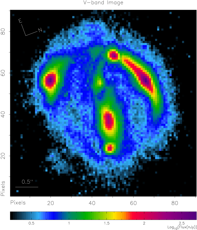
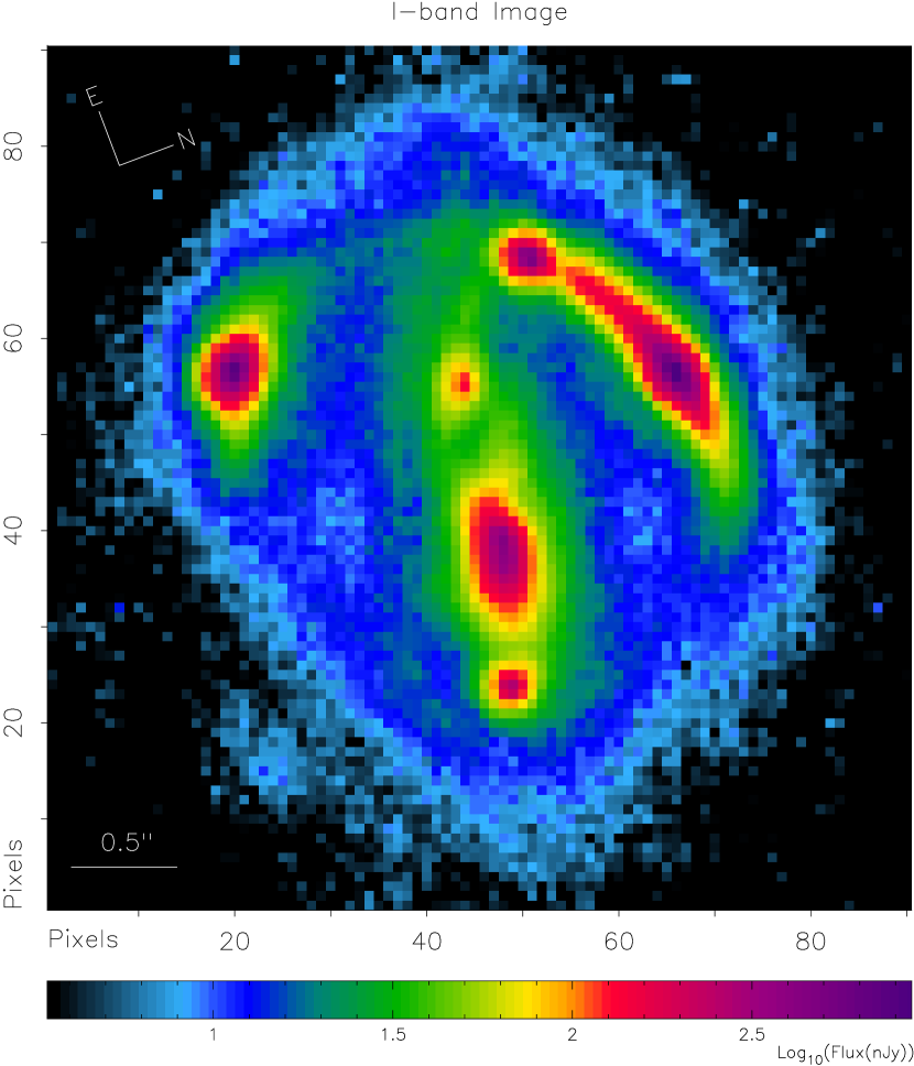
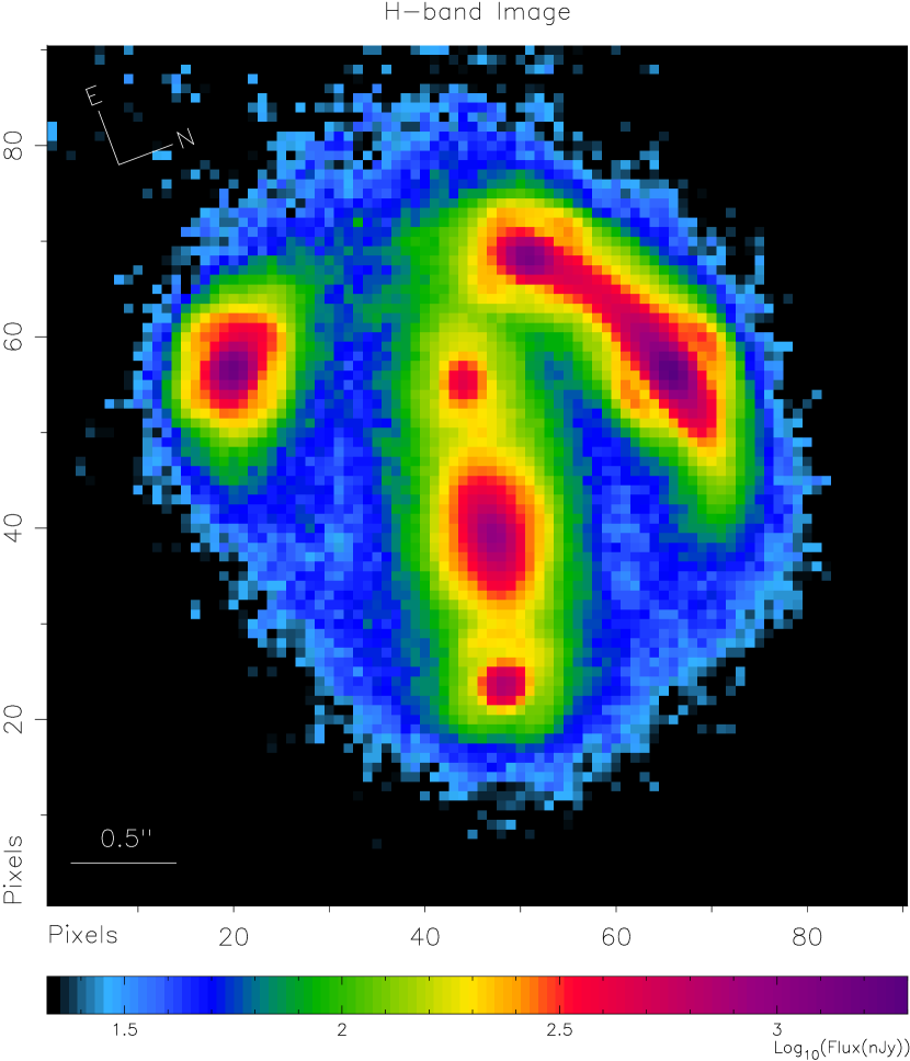
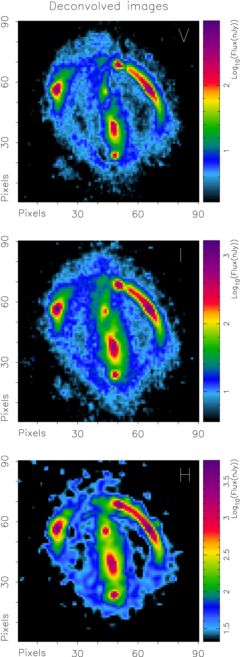
The final V, I, and H band images are shown in Figures 1, 2 and 3. The orientation of the images is the original orientation of the V and I frames (notice that north is not up). The intensity is in logarithmic units of nJy per pixel, and only fluxes above 3 are displayed, where and 6 nJy are the mean standard deviation of the sky noise in V, I, and H bands respectively. The H band image is the most affected by PSF convolution, as shown by the clearly defined diffraction rings surrounding A, C, and D components in Fig. 3. With a source redshift , the filters F606W (V band), F814W (I band) and F160W (H band) correspond to source emission at mean rest-frame wavelengths of 2506Å, 3340Å and 6713Å, respectively. Similarly, for the lens galaxies located at , we are observing the emission from 3882Å, 4905Å and 9860Å in their rest frame. The centroids of the four components of the source A, B, C, and D, and the lensing galaxies G1 and G2 in each band are listed in Tab. 3.
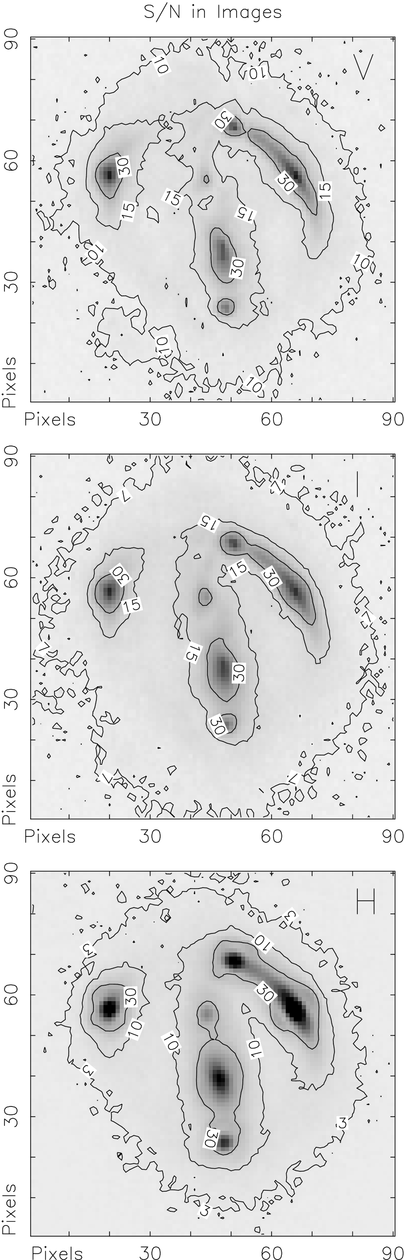
We evaluate the signal-to-noise in the images on a pixel-by-pixel basis. In the V and I images the noise is estimated from contributions of Poisson, readout and background noise. In H band the background noise changes from frame to frame, and also across each frame, so we determine the noise using the dispersion of the data at each pixel. Contours of constant signal-to-noise for the images are plotted in Fig. 4. In general V and I band have approximately the same level of S/N. Compared to H, the S/N in V and I is higher in low emission regions. For example, low emission at 3 level has S/N10, 7 and 3 in V, I, and H images respectively. Isophotes enclosing 50% of the source flux have approximately S/N 30 in the three bands, and isophotes enclosing 10% of the source flux have S/N 70, 70, 150 in the V, I, and H band respectively.
All bands reveals the extended structure of B1608+656, showing the four multiple images of the background source embedded in a ring-like emission surrounding the two lens galaxies. There are qualitative differences between the extended emission of the images, however. First the saddle point that indicates the boundary between C and A images is closer to image C in V and I-band than in H-band. Since the separation between A and C is determined by the critical curve associated with the lens potential, it should not depend on the wavelength. The shift of 0.16” in the observed saddle point can be a consequence of extinction, PSF convolution, or a combination of both. If the shift is mainly due to high extinction near C, then the actual saddle point would lie closer to H location. On the other hand, if the shift is due to the prominent PSF Airy ring in H band around image C, then the actual saddle point would lie closer to its location in V and I band. When the extended structure of the source is incorporated into the modeling of the system (Blandford, Surpi & Kundić, 2001), the saddle points between multiple images (or flux minima in the Einstein ring) can place strong constraints on the lens potential. However, until the images are corrected for extinction and PSF distortions, the uncertainty in the location of the saddle point mentioned above can possibly lead to wrong conclusions if used to constrain or confront lens models as attempted by Kochanek, Keeton & McLeod (2001).
The second qualitative difference between the images is that the centroid of the lens galaxy G1 appears to shift at decreasing wavelength in, approximately, the west direction. The G1 centroid is displaced by 0.085” in V band, and by 0.073” in I band, with respect to its H band location (see Tab. 3). There are two possible explanations. One is that the east part of the galaxy is being reddened, in which case the G1 centroid would lie closer to its H band position. The other explanation, proposed by Koopmans & Fassnacht (1999), is that the shift is a consequence of a change in the intrinsic color of G1. These authors propose that dynamical interaction of G1 and G2 could create a bluer region of star formation close to the centroid of G1 in V band, and that this centroid would then represent the center of mass of the lensing galaxy. This interpretation supports their best fitting lens model, which was obtained using the centroid of G1 in V band as a constraint. However, until we understand the origin of the shift of the G1 center as a function of the wavelength, its use to constrain lens models can lead to erroneous conclusions. We should notice at this point that the centroid of G1 is not alone in changing from one band to another; the centroids of G2, D, and C also shift as can be seen from Tab. 3.
The main conclusion is that a correct interpretation of the features observed in the extended structure of the background source and lens galaxies at V, I, and H bands requires further study of the PSF convolution, intrinsic color variation and extinction in the system. We discuss these effects in the next sections.
| V-band | I-band | H-band | |
|---|---|---|---|
| A | 65.740.05 56.620.06 | 65.840.04 56.550.05 | 65.640.03 56.510.03 |
| B | 19.880.05 56.570.06 | 19.940.04 56.600.05 | 19.920.03 56.620.03 |
| C | 50.570.07 68.500.07 | 50.670.05 68.400.05 | 50.920.04 68.310.03 |
| D | 48.720.10 23.810.10 | 48.790.07 23.830.07 | 48.320.04 23.630.04 |
| G1 | 48.020.06 37.550.13 | 47.980.04 37.830.09 | 47.180.04 39.220.05 |
| G2 | 43.500.19 55.470.27 | 43.620.10 55.330.14 | 44.130.06 55.260.07 |
4 SOURCE POST-STARBURST POPULATION
An optical spectrum of the background source in B1608+656 was obtained with the double spectrograph on the Palomar 5 m telescope by Fassnacht et al. (1996), by positioning the slit so as to minimize the lens galaxies light. The spectra showed prominent high-order Balmer absorption lines and Mg II absorption, allowing the determination of a conclusive redshift of for the source, and indicating it is a post-starburst or E+A galaxy. No emission associated with the AGN was found. Comparing photometry of the source through the filters F555W, F606W, F814W and F160W with isochrone synthesis models of Bruzual & Charlot (1993) we find that the post-starburst population in the host galaxy is around 500 Myr old. Fig. 5 shows photometry of the B component of the source within an elliptical aperture of radius 0.3”, superposed on the spectrum model. There is a remarkable agreement of the photometry points with the model. The same fit is found for photometry in different areas of B, as this image shows no significant change of color. When the optical spectrum of the source in Fassnacht et al. (1996) is compared with the model, we find the absorption lines and overall shape of the continuum of the source are fitted well by the 500 Myr old instantaneous burst model of Bruzual & Charlot (1993) as showed in Fig. 6, confirming the age estimation.
This model can set an upper limit to the age of the starburst population in the source. Older starbursts would be redder than the source, and are ruled out since no mechanism would be able to account for the discrepancies. On the other hand, younger starburst models, if reddened or combined with older stellar components, could still fit the source. We experimented with a younger starburst subject to extinction or superposed on older populations but the fit to the spectrum and photometry of the source was inferior. We adopt the 500 Myr old instantaneous starburst model to describe the stellar population at the source in what follows. The model provides a synthetic spectrum for the source in the violet end of visible light and infrared where no direct observations are available. The spectrum is used in the next section to generate the PSFs of the V, I, and H filters.
5 IMAGE DECONVOLUTION
In this section we present initial deconvolutions of the V, I, and H band images. We use the Tiny Tim software package to generate HST model Point Spread Functions (Krist & Hook, 1999)222Tiny Tim User’s Guide is available at: http://www.stsci.edu/software/tinytim, and the Lucy routine in IRAF (STSDAS, 2001)333Space Telescope Science Data Analysis System is available at: http://ra.stsci.edu/STSDAS.htmlto deconvolve the images. This task restores images using the Lucy-Richardson method (Lucy, 1974) adapted for HST images contaminated with Poisson noise.
HST PSFs comprise a core, diffraction rings and radial spokes. Their shape is dominated by diffraction rather than seeing effects, and the PSFs appearance changes at increasing wavelength as the diffraction patterns expand proportionally. In broad-band filters, as F606W, F814W, and F160W, the superposition of the monochromatic Airy rings at the different wavelengths of the bandpass results in PSFs with smooth wings. The generation of these polychromatic PSFs requires knowledge of both the transmission function of the filter and the spectrum of the observed object. We use the database of wavelength and weights supplied by the Tiny Tim package for the transmission of each filter, and the 500 Myr old instantaneous starburst model from Bruzual & Charlot (1993) to characterize B1608+656 spectrum.
PSFs are constructed with a resolution of 0.011” by subpixelizing with a factor 4 in each dimension. We subpixelize the images by the same factor using linear interpolation and deconvolve them with the Lucy routine in IRAF (STSDAS, 2001)5. The criterion adopted for convergence was to increase the number of iterations until the deconvolved image convolved with the PSF reproduced the observed image within an error of 5%. Many light distributions are, after convolution with the PSF, compatible within a 5% error with the observed image. It is expected then that the difference between the deconvolved image and the original light distribution is higher than 5%. After deconvolution the images were repixelized to its original resolution. The deconvolved images are shown in Fig. 7. The H band image is the most difficult one to deconvolve, since the diffraction rings are very prominent. Residuals of the rings are still present around A, C, and D in the deconvolved H image. The H deconvolution did not solve for the uncertainty in the saddle point between A and C components. The arc in the deconvolved H image now shows two minima, one at each side of the intersection between the remnants of the Airy ring around C and the arc. The two locations correspond approximately to the position of the minima in V and I, and the minima in H before deconvolution.
We should stress here that deconvolution is not a unique operation, and the images presented here are the best results obtained under certain limitations: (i) The model assumed for the spectrum is known to fit the observed spectrum of the source, which lies between 6000 Å and 9600 Å . If the extrapolation of the model toward lower and higher wavelengths has local discrepancies with the spectrum of the source, the restoration in V and H bands might be limited. (ii) The spectrum was assumed constant. It was modeled after the source to obtain better results in the deconvolution of the four images of that object. However, as the result of contamination with light from the lens galaxies and extinction, the color does change across the frame as we will show in the next section. (iii) Even for sources of known constant color, deconvolutions are limited by the accuracy of the algorithms used to deconvolve. We tried an alternative deconvolution method, the Maximum Entropy Method (MEM package in IRAF (STSDAS, 2001)5), and found similar results, except that it produced a slightly higher noise level. The creation of artifacts by the amplification of the noise is the principal illness of the standard methods for deconvolution.
6 EXTINCTION AND COLOR MAPS
The three HST images have different angular resolutions because they were convolved with different PSFs during observation. The deconvolution probably has restored the images to comparable resolution, but has also amplified their noise. Using the deconvolved images to create the color maps results in maps which are dominated by pixel-scale structure. However, the extinction is an average over a galactic scale length along the line of sight, so it ought to vary relatively slowly across the galaxies. The small scale structure observed has to be artificial, due to noise that propagates from the deconvolved images. To reduce the noise in the color maps, instead of using deconvolved images, for our analysis we created images of comparable resolution by further convolving each image. At each band we create a PSF, given by the ratio (in Fourier space) between a Gaussian PSF with =1.5 pixels, and the PSF of the corresponding filter. The convolution of the observed images with the “PSFratio” results in images of comparable resolution, equivalent to the original images convolved with the Gaussian PSF. In this section we will use V, I, and H band images that have been subjected this procedure.
A preliminary inspection of the relative magnifications of components A, B, C, and D at H, I and V bands reveals increasing extinction as we move to shorter wavelengths. We select the brightest pixels in image B at each band. These pixels are delimited by an isophote of ellipticity 0.34 and semi-major axis of 0.3”, and enclose fluxes of 6.90, 14.5 and 57.6 Jy at V, I, and H band respectively (which is approximately 50% of the total flux in component B). Since image B is the furthest away from G1 and G2, we assume that it is the least reddened and we compute the extinction of A, C, and D relative to B. Assuming the measured radio flux ratios (listed in Tab. 1) are correct we take the brightest pixels, with for A, C, and D. These pixels cover matching areas at the source and their relative fluxes should reproduce, in absence of extinction, the observed radio magnifications. For example, at V band the pixels selected at A should add to flux JyJy. We compute the relative extinction at each component as , where H, I and V and is the flux measured in the selected patch. The values are listed in the Tab. 4 and show that A suffers little extinction, while C and D are strongly reddened relative to B.
| A | B | C | D | |
|---|---|---|---|---|
| 0.08 | 0.0 | 0.14 | 0.20 | |
| 0.08 | 0.0 | 0.43 | 0.42 | |
| 0.12 | 0.0 | 0.69 | 0.71 |
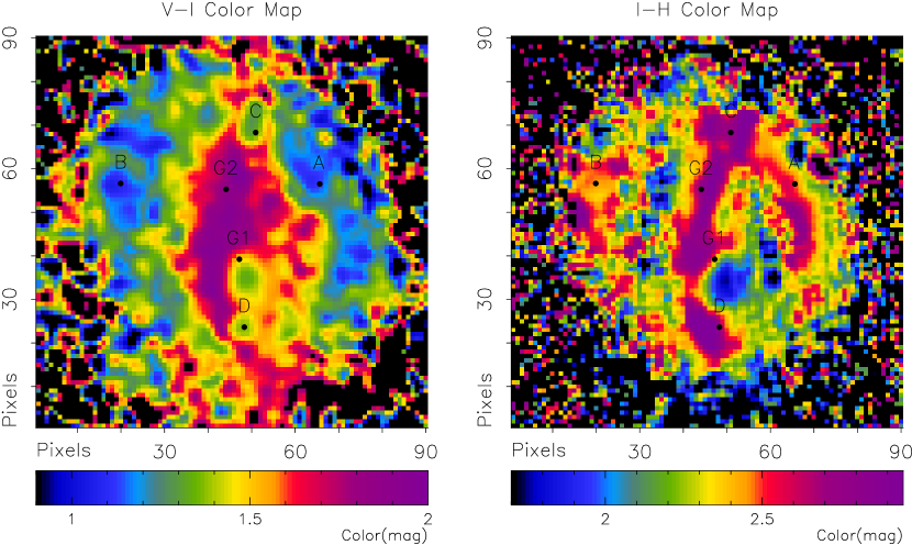
There are two independent colors, which we choose to be VI and IH. We use Vega: magnitudes m=, where CR is the count rate (measured counts per second) and the zero point ZP=21.49, 21.64, 22.89 for F160W, F814W, F606W respectively (STScI, 1998). Colors are then evaluated pixel by pixel as VI and IH, where images are in CR units. VI and IH colors are shown in Fig. 8. The orientation of the color maps is as in the Figures 1, 2 and 3, so that north is not up. To avoid confusion we will use up-down-left-right to locate features in the maps.
Color gradients in Fig. 8 can arise from two different effects, extinction or variation in the intrinsic color of the objects. At first sight, there is an overall pattern in the color. Both maps show maximum values in a vertical stripe compromising C, G2, G1 and D. A change of color in C and D (with respect to A and B) was expected since both images are highly reddened. In G1 and G2 area, the stripe is broader in V-I than in I-H map, showing the lenses have different intrinsic color than the source. Contamination of C and D with light from the lens galaxies could also be contributing to their change of color respect to A and B. Estimated colors within an elliptical aperture of radius 0.3” in B and matching areas in A, C, and D are reported in Tab. 5. In VI map the color shows larger gradients across the components and minimum and maximum values are listed in Tab. 5, while IH colors reflect average values.
| Color(mag) | A | B | C | D |
|---|---|---|---|---|
| VIaaColors are minimum and maximum values measured within an elliptical radial aperture of 0.3” in B, and matching areas in A, C, and D. | 1.10-1.50 | 1.06-1.28 | 1.28-1.60 | 1.38-1.51 |
| IHbbColors correspond to mean values within the same apertures. | 2.52 | 2.47 | 2.70 | 2.48 |
The maps in Fig. 8 have color variation across the lensing galaxy G1. There is a minimum of color centered approximately at pixel (49,34), and an steep color gradient toward the upper-left direction. Minimum and maximum colors observed in G1 area are tabulated in Tab. 6. The bluer region of G1 does not correspond to the nucleus of the galaxy, it is located 0.25”, 0.18” and 0.17” off the centroid of the surface brightness distribution in H, I and V bands respectively (see Tab. 3). But, if the two lensing galaxies were interacting dynamically creating a region of star formation in that area, the change of color could still be interpreted as intrinsic to G1 as suggested by Koopmans & Fassnacht (1999). However, photometry through the bluer window shows that region is not singular and follows a clearly defined de Vaucouleur profile (Blandford, Surpi & Kundić, 2001) identifying G1 as an elliptical galaxy. The photometry also indicates that G1 is bluer than the average spectral energy distribution of normal ellipticals (see for example (Schmitt et al., 1997)). This would agree with the hypothesis of Myers et al. (1995) that the lens might also be a post-starburst galaxy, based on the absorption lines observed in the spectrum. We conclude that the color variations in G1 do not reflect a change of its intrinsic color but differential extinction. The extinction is probably due to dust associated with G2, since ellipticals usually contain little or no dust. The reddest area in Fig. 8 shows the extinction by dust G2 has probably left behind when it swung around G1. On the basis of these color maps we conclude that the dust now associated with G2 must extinguish more than half of the light of G1, implying that the dust is closer to us than G1. Although it is possible to contrive different models the most natural expectation is that galaxy G2 has a smaller redshift than G1. Either way a measurement of and would be most instructive.
The minimum colors quoted in Tab. 6 for G1 are seen through the lower reddening area and place an upper limit on G1’s intrinsic color (a constant reddening over G1 can still be taking place modifying its photometric color). Combining these values with the maximum colors reported we estimate G1 color excess , and in a similar way. G1 colors were also extracted by Kochanek et al. (2000); they found and (not corrected for extinction), with V corresponding to F555W. ¿From Tab. 6 we find mean values and . The discrepancy between the VH values is probably because the V band corresponds to different filters, F606W (here) and F555W (in citation). We don’t expect the colors to agree perfectly for two further reasons. First, the G1 color varies across the source and the average used here might differ from the one used in Kochanek et al. (2000). Second we estimate colors after convolving the images with the corresponding PSFratio, while in Kochanek et al. (2000) images have not been convolved. We remark that mean colors are not representative of G1 intrinsic color, nor of its reddened color, but just of its average.
In the case of G2, the color also varies across the galaxy. G2’s photometric centroid differs in each band, the centroid shifts approximately to the left direction at decreasing wavelength. The I band centroid is shifted by 0.023”, and V centroid by 0.030”, from H centroid (see Tab. 3). This suggests that the extinction is higher in the right part of the galaxy. The color maps in Fig. 8 show a redder area around pixel (46,56) which is 0.1” to the right from G2 mean centroid in V, I, and H, likely to be a region of maximum extinction in G2 rather than a redder intrinsic color. We then interpret the variation of color observed in G2 as mainly due to extinction, and once again the minimum and maximum colors observed give indications of the intrinsic color and the most reddened area respectively. G2 colors are reported in Tab. 6, and from them we estimate and . Since G2 is abundant in dust, it is probably a late type galaxy, highly distorted due to its encounter with G1.
| Color(mag) | G1 | G2 |
|---|---|---|
| VIaaColors are minimum and maximum values measured. | 1.34 - 1.97 | 1.67 - 2.00 |
| IHaaColors are minimum and maximum values measured. | 1.77 - 2.87 | 2.10 - 2.94 |
The color maps showed in Fig. 8 have two different sources of error. First, noise coming from the V, I, and H band images (see Fig. 4). For the VI map it can be estimated as , and similarly for the IH map. This noise decreases at increasing signal and it will mainly compromise the restoration of the low emission regions. The second uncertainty in the color maps comes from the two PSF convolutions, one during the observation and the second performed here. The noise pattern they produce is opposite to the previous one, with the noise increasing at increasing signal in the images. The degradation due to the convolutions is significant and the only way of dealing with it is to apply the color maps to images with the same resolution, i.e. images that have been treated with the same convolution process.
7 DISCUSSION
The V, I, and H band HST images of B1608+656 show Einstein ring emission from the four images of the radio source, encircling the two lens galaxies. Pixel photometry indicates qualitative differences between the emission in the three bands, arising from extinction and PSF convolution. It is immediately apparent from V-I and I-H color maps that most of the reddening is due to dust associated with the lens galaxy G2, probably a late type galaxy, which has been gravitationally swung around by the other lens galaxy, G1, an elliptical. The extinction most strongly affects G2, the east portion of G1, and two of the four multiple images of the source, the ones nearly aligned with the position angle of the lenses. Of the three bands, H is the most affected by PSF convolution. The H band image shows prominent Airy rings around the multiple images, and is the most difficult to restore. The H band image in NIC2, from CASTLES, suffers from the same problem. Additional infrared imaging with a large ground based telescope equipped with adaptive optics would be worth pursuing.
There are multiple features that can be seen in the extended emission and used as constraints to break the degeneracy of current lens models: (i) the location and radial profile of the lens galaxies (which are not observed in the radio), (ii) special properties of the Einstein ring like saddle points, traces of the critical curve, and the inner and outer limits where quad images are formed, and (iii) the overall ring surface photometry, which satisfies a four-to-one mapping into the source plane. However, the strong extinction in V and I bands, the significant PSF distortion in H band, and the contamination of the ring with emission from the lens galaxies make clear that the images need to be corrected before being used as constrains, or they could lead to misleading conclusions. The multi-wavelength strategy required to correct the images will be applied in Paper2, but it can be schematized here based on the observations we made above. First, images have to be taken to comparable spatial resolution. The extinction can then be measured from the color maps constructed with them. If current methods for deconvolution are applied, as these techniques amplify the noise in the images, the deconvolution should be done after the images have been corrected for extinction. PSF deconvolution and the measurement of extinction require knowledge of the intrinsic color of the source, and yield better results if applied to a source of constant color, so that a decomposition of the surface photometry into emission from the lens galaxies and the source host galaxy, should precede them.
Appendix A APPENDIX: V AND I-BAND IMAGE PROCESSING
We process here the set of HST archival exposures from proposal 6555, taken in 1997 November using the planetary camera PC1 of the WFPC2 instrument, through the filters F606W and F814W (see Tab. 2). The PC1 has a pixel size of 0.0455” and a format of 800x800 pixels. Pixel data are converted from DN counts units into electrons multiplying by the factor of Gain=7e-DN-1. Each e- corresponds to one photon detected. Beyond the quantum efficiency, the efficiency of each WFPC2 exposure is limited by the photon count noise , the instrument read-out noise , and the sky background noise . The standard deviation at each pixel is then . For the WFPC2 the read-out noise standard deviation is . Photon counts result from a Poisson process in which the standard deviation can be estimated as the square root of the signal in photon counts S. The signal-to-noise of the image then equals . The S/N will approximately grow linearly with the signal strength for , and then as the square-root of the signal, as the Poisson noise in the object begins to dominate over the sky and read-out noise. Notice that in the last regime the S/N increases as the square root of the exposure time.
There are eight frames in proposal 6555, hereafter designated as f1,f2… f8 according to the time order they were observed. Frames f1, f2, f5 and f6 were taken using the F814W filter and frames f3, f4, f7 and f8 with the F606W filter. We measure and subtract the mean sky level at each frame. The values obtained are listed in Tab. 7. V frames have a mean sky level of photons. The standard deviation of photons results from the combination of photons, photons, and photons. We find the I frames have a mean sky background of photons which yields photons.
| Frame | Band | Sky LevelaaSky measured in units of photons. | Multi-pixel ShiftbbThe two values correspond to x and y shifts in the pixel grid. | Sub-pixel ShiftbbThe two values correspond to x and y shifts in the pixel grid. |
|---|---|---|---|---|
| f1 | I | 23.3 9.9 | +5 +5 | +0.05 -0.21 |
| f2 | I | 26.6 10.0 | +5 +5 | +0.08 -0.24 |
| f3 | V | 49.4 11.8 | +5 +5 | -0.13 +0.21 |
| f4 | V | 49.0 11.8 | +5 +5 | -0.10 +0.20 |
| f5 | I | 27.9 10.1 | +0 +0 | +0.10 -0.20 |
| f6 | I | 26.5 10.1 | +0 +0 | +0.11 -0.20 |
| f7 | V | 47.8 11.8 | +0 +0 | -0.06 +0.21 |
| f8 | V | 48.6 11.7 | +0 +0 | -0.06 +0.22 |
All the input frames in F606W and F814W are registered together before performing the average in each filter. We first perform the multi-pixel shifts listed in Tab. 7. Prior to determine the sub-pixel shifts, bad pixels and cosmic rays are replaced with median values at each frame. We use component B in B1608+656 and a star located at from B as references to determine sub-pixel shifts relative to f1 by cross-correlating the frames. Since the error introduced in a shift increases with the amount shifted, we re-normalize our shifts to the minimum possible values. This also keeps the resolution in the frames comparable. The (renormalized) sub-pixel shifts applied are listed in Tab. 7.
The frames are contaminated with bad pixels and cosmic rays. To clean them before performing the average we create a pixel mask for each frame rejecting bad pixels and pixels above and below 3 level of the signal. For the thresholding we estimate the signal S with the median, and S, with the above determined. After averaging the frames with weights according to their exposure time, we arrive at the final V and I images shown in Figs. 1 and 2. We create signal-to-noise maps evaluating on a pixel-by-pixel basis, where n is the number of frames contributing to the average at each pixel after masking. Contours of constant S/N=10, 15 and 30 in V, and S/N=7, 15 and 30 in I are plotted in Fig. 4.
Appendix B APPENDIX: H-BAND IMAGE PROCESSING
In this appendix we process HST infrared imaging of B1608+656 obtained with the NIC1 camera through the filter F160W. The observations were conducted in 1997 February as part of HST proposal 7422. The NIC1 detector is an array of 256x256 pixels whose elements are divided into four independent quadrants of 128x128 pixels. The pixel size is 0.043” and the conversion from pixel data in DN = counts/sec into electrons/sec is determined by the factor of Gain=5e-DN-1. There are 7 exposures with F160W, designated h1, h2.. h7 in chronological order. The first five exposures are 3839.94 seconds long, h6 is 2047.86 seconds long, and h7 is 895.92 seconds long.
The images suffer from some typical anomalies of NIC1. All frames present the NIC1 high noise region in the upper left quadrant. This region has a sensitivity that is factor of 2-3 lower than the mean of the array and its noise gets highly amplified during the calibration process. The lens is located in the lower right quadrant, but is still marginally affected by the high noise region. The second anomaly present in all frames is the bad central row, which affects all pixels in row 128 of the array and sometimes the adjacent rows as well. The lens extends over row 128 in frames h3 and h6. We therefore discard rows from 126 to 130 in those frames. We also discard rows 127 to 129 that can marginally affect the area around the lens in all frames. There is also evidence for quadrant dependence of the signal, which is not unexpected since each quadrant has its own amplifier. This can be relevant in h3 and h6 where the lens extends over two quadrants. Frame h6 does not seem to be affected, but the signal in the north right quadrant of h3 has higher amplification than the rest of the frame and the data in that quadrant will not be included. The frames also show evidence of glow or maximums in the corner of each quadrant, due to the readout amplifiers, but that doesn’t seem to affect the lens area.
The sky is very noisy, its level differs from frame to frame, and it also varies across each frame. With the high noise region of NIC1 located in the north-left quadrant, and B1608+656 in the lower-right quadrant, the noise creates a sky level in the lens area that can be modeled as a gradient at -45o direction (degrees counterclockwise from +y pixel coordinates). The noise level follows the same pattern. We first determine the mean sky level in the lower-right quadrant of NIC1 and subtract it. These values are listed in the second column of Tab. 8. Then we model the remaining sky gradient as , where x and y are pixel coordinates and C is a constant. The fitted values of C are listed in Tab. 8.
| Frame | Sky LevelaaSky measured in units of photons. | Sky Gradient Ca,ba,bfootnotemark: | Pixel ShiftccThe two values correspond to x and y shifts in the pixel grid. | Weight Factor |
|---|---|---|---|---|
| h1 | 714 242 | 0.0028 | 22.91 22.78 | 0.31 |
| h2 | 402 136 | 0.0017 | -0.10 22.74 | 0.56 |
| h3 | 96.7 88.2 | 0.0001 | 22.95 -0.32 | 0.86 |
| h4 | 154 76.0 | -0.0002 | 46.14 23.09 | 1.0 |
| h5 | 96.2 87.1 | -0.0022 | 23.08 46.42 | 0.87 |
| h6 | 38.3 46.0 | -0.0013 | -0.24 -0.23 | 0.87 |
| h7 | 10.7 31.1 | -0.0002 | 46.24 46.52 | 0.56 |
Using the centroids of A, B, C, D and G1 we determine the relative shifts between frames, but we don’t apply them yet (the values are listed in Tab. 8). H frames need a further rotation, translation and magnification to be registered to the V and I pixel grid. At this point it is better to register the H frames directly to the V and I grid before the combination. This involves only one geometrical transformation, while shifting, combining and registering the final H image to V and I involves two. Using A and B centroids we determine a rotation of 7.903o (degrees counterclockwise) is needed to register H frames to V and I. A magnification factor of 1.05819 is also required because H frames have 0.043” pixels while V and I frames have 0.0455” pixels. Combining all this information we determine the transformation needed to register each H frame to the V and I grid of pixel coordinates.
There is no contamination with cosmic rays, as they have been filtered out by use of MULTIACCUM mode. Only a few bad single pixels need to be rejected. We average the frames using weights to account their different exposure time and background noise error, the weight factors used are listed in Tab. 8. The resulting H image is shown in Fig. 3. The S/N in the image is hard to characterize. The statistical properties of the noise can be affected by the rotation and re-scaling performed to the individual frames. Besides, even before the registration, the difference between the background noise in the frames makes the general formula used to estimate the S/N for V and I bands not appropriate. We construct here a S/N map estimating the noise from the standard deviation in the data at each pixel, appropriately smoothed. Contours of S/N=3,10 and 30 are shown in Fig. 4.
References
- Blandford & Kundić (1996) Blandford, R. D., & Kundić 1996, in The Extragalactic Distance Scale, ed. M. Livio, M. Donahue & N. Panagia (Cambridge: Cambridge University Press), 60
- Blandford, Surpi & Kundić (2001) Blandford, R., Surpi, G., & Kundić, T. 2001, in ASP Conf. Ser. 237, Gravitational Lensing: Recent Progress and Future Goals, ed. T. G. Brainerd & C. S. Kochanek (San Francisco: Astronomical Society of the Pacific)
- Bruzual & Charlot (1993) Bruzual, G., & Charlot, S. 1993, ApJ, 405, 538
- CASTLES (2001) CASTLES, Cfa-Arizona Space Telescope LEns Survey, on-line Gravitational Lens Data Base
- Fassnacht et al. (1996) Fassnacht, C. D., Womble, D. S., Neugebauer, G, Browne, I. W. A., Readhead, A. C. S., Matthews, K., & Pearson, T. J. 1996, ApJ, 460, L103
- Fassnacht et al. (1999) Fassnacht, C. D., Pearson, T. J., ReadHead, A. C. S., Browne, I. W. A., Koopmans, L. V. E., Myers, S. T., & Wilkinson, P. N. 1999, ApJ, 527, 498
- Fassnacht et al. (2001) Fassnacht, C. D., Xanthopoulos, E., Koopmans, L. V. E, Pearson, T. J., Readhead, A. C. S., & Myers, S. T. 2001, in ASP Conf. Ser. 237, Gravitational Lensing: Recent Progress and Future Goals, ed. T. G. Brainerd, & C. S. Kochanek (San Francisco: Astronomical Society of the Pacific)
- Jackson et al. (1997) Jackson, N. J., Nair, S., Browne, I. W. A. 1997, in Observational Cosmology with the New Radio Surveys, eds., M. Bremer, N. Jackson & I. Perez-Fournon, (Dordrecht: Kluwer), 315
- Kochanek et al. (2000) Kochanek, C. S., Falco, E. E., Impey, C. D., Léhar, B. A., McLeod, B. A., Rix, H. W., Keeton, C. R., Muñoz, J. A., & Peng, C. Y. 2000, ApJ, 543, 131
- Kochanek, Keeton & McLeod (2001) Kochanek, C. S., Keeton, C. R., & McLeod, B. A. 2001, ApJ, 547, 50
- Koopmans & Fassnacht (1999) Koopmans, L. V. E., & Fassnacht, C. D. 1999,ApJ, 527, 513
- Krist & Hook (1999) Krist, J., & Hook, R. 1999, in The Tiny Tim User’s Guide, on-line documentation
- Lucy (1974) Lucy, L. B. 1974, AJ, 79, 745
- Myers et al. (1995) Myers, S. T. et al. 1995, ApJ, 447, L5
- Refsdal (1964) Refsdal, S. 1964, M.N.R.A.S., 128, 307
- Snellen et al. (1995) Snellen, I. A. G., Bruyn, A. G., Schilizzi, R. T., Miley, G. K., & Myers, S. T. 1995, ApJ, 447, L9
- Surpi & Blandford (2001) Surpi, G., & Blandford, R. 2001, in ASP Conf. Ser. 237, Gravitational Lensing: Recent Progress and Future Goals, ed. T. G. Brainerd, & C. S. Kochanek (San Francisco: Astronomical Society of the Pacific)
- Schmitt et al. (1997) Schmitt, H. R., Kinney, A. L., Calzetti, D., Storchi Bergmann, T. 1997, AJ, 114, 592
- STScI (1998) STScI, Space Telescope Science Institute 1998, HST Data Handbook 3.1, Chapter 28, Table 28.1
- STSDAS (2001) STSDAS, Space Telescope Science Data Analysis System, on-line documentation
- Walsh, Carswell & Weymann (1979) Walsh, D., Carswell, R. F., & Weymann, R. J. 1979, Nature, 279, 381