Cosmic Microwave Background Anisotropy
in models with Quintessence

Abstract

We study the Cosmic Microwave Background (CMB) anisotropies produced by cosine-type quintessence models. In our analysis, effects of the adiabatic and isocurvature fluctuations are both taken into account. For purely adiabatic fluctuations with scale invariant spectrum, we obtain a stringent constraint on the model parameters using the CMB data from COBE, BOOMERanG and MAXIMA. Furthermore, it is shown that isocurvature fluctuations have significant effects on the CMB angular power spectrum at low multipoles in some parameter space, which may be detectable in future satellite experiments. Such a signal may be used to test the cosine-type quintessence models.

TU-638

Department of Physics, Tohoku University
Sendai 980-8578, Japan

1 Introduction

Recent cosmological observations suggest that there exists a dark energy which must be added to the matter density in order to reach the critical density. Although the cosmological constant is usually assumed as the dark energy, in the past years, a slowly evolving scalar field, dubbed as “quintessence” has been proposed as the dark energy [3] and has been been studied by many authors [4]. There are some differences between the cosmological constant and quintessence. Firstly, for the quintessence, the equation-of-state parameter $\omega_{Q}=\rho_{Q}/p_{Q}$ varies with time, whilst for the cosmological constant, it remains a fixed value $\omega_{\Lambda}=-1$. Secondly, since the quintessence is a scalar field, it fluctuates.

One of the observational effects produced by the existence of the quintessence is the CMB anisotropies. In many cases, the quintessence dominates the universe at late times ($z\sim O(1)$, with $z$ being redshift) after the recombination. At that epoch the gravitational potential is changed because the equation of state for quintessence is different from that for non-relativistic matter, which leads to an enhancement of the CMB anisotropies at large angular scales $l\lesssim 10$ due to the late-time integrated Sachs-Wolfe effect. The quintessence also changes the locations of the acoustic peaks in the CMB angular power spectrum because the projection of the horizon at last scattering onto the present sky is enlarged compared with models with the cosmological constant. Furthermore, the initial fluctuations of the quintessence fields are generated during inflation. These fluctuations behave as isocurvature mode [5] and hence the quintessence may have both adiabatic and isocurvature perturbations.

2 CMB anisotropy in models with cosine-type quintessence

The quintessence model we take here is the cosine-type quintessence which has the potential

$$V(Q)=\Lambda^{4}\left[1-\cos\left(\frac{Q}{f_{Q}}\right)\right]=2\Lambda^{4}\sin^{2}\left(\frac{Q}{2f_{Q}}\right),$$ (1)

where $f_{Q}$ and $\Lambda$ are model parameters. This type of potential can be generated if the quintessence field is a pseudo Nambu-Goldstone boson. In this class of models, effective mass of the quintessence field is always of $O(\Lambda^{2}/f_{Q})$.

Since the quintessence is a scalar field, its amplitude may have position-dependent fluctuations. To investigate its behavior, we decompose the $Q$ field as $Q(t,\vec{x})=\bar{Q}(t)+q(t,\vec{x})$, where $q$ is the perturbation of the amplitude of the quintessence field. Before we consider the fluctuations of the quintessence fields, we discuss the dynamics of the zero mode of the quintessence fields briefly. For details, see Ref.[1].

The zero mode $\bar{Q}$ obeys the equation of motion $\ddot{\bar{Q}}+3H\dot{Q}+dV/dQ=0$ where the dot represents the derivative with respect to time $t$. When the relation $H\lesssim\Lambda^{2}/f_{Q}$ is satisfied, the quintessence field starts to oscillate. If the combination $\Lambda^{2}/f_{Q}$ is large, the oscillation starts earlier epoch and the quintessence field undergoes many oscillations until the present time. We call the parameter space where the oscillation of the quintessence is significant as “oscillatory region.” When the quintessence field starts to oscillate earlier, it dominates the energy density of the universe from earlier epoch. This has significant implications to the CMB power spectrum.

Now we discuss the the fluctuations of the quintessence fields. There are two origins of non-vanishing $q$ at the present time; one is non-vanishing gravitational potential $\Psi$ and the other is primordial $q$ itself. We call these modes as “adiabatic” and “isocurvature” modes, respectively. In the actual situations, both modes may exist. Since these modes are uncorrelated, the total fluctuation can be decomposed into two modes which originate to primordial fluctuations in $\Psi$ and $q$, respectively:
$\displaystyle{\rm Adiabatic}:\left\{\begin{array}[]{l}\Psi(a\rightarrow 0)\neq 0\\ q(a\rightarrow 0)=0\end{array}\right.,$ (3) $\displaystyle{\rm Isocurvature}:\left\{\begin{array}[]{l}\Psi(a\rightarrow 0)=0\\ q(a\rightarrow 0)\neq 0\end{array}\right..$ (6)
We assume that there is no entropy fluctuations between any of two energy components other than that of quintessence. Thus, the adiabatic mode given with the initial condition (6) corresponds to the conventional adiabatic initial condition. On the contrary, the mode with the initial condition (6) is called “isocurvature mode,” since the total density fluctuation and the potential $\Psi$ vanishes as $a\rightarrow 0$ if this is the only source of the fluctuation in the early universe. To parameterize the relative size of adiabatic and isocurvature contributions, it is convenient to define $r_{q}$, the ratio of the primordial value of $\tilde{q}$ to that of the gauge-invariant variable $\tilde{\Psi}$ at the radiation-dominated universe

$$r_{q}\equiv\frac{\tilde{q}}{M_{*}\tilde{\Psi}},$$ (7)

where $M_{*}$ is the reduced Planck scale. Since the ratio $r_{q}$ generically depends on the model of the inflation, we treat $r_{q}$ as a free parameter in our analysis. (For example, for the chaotic inflation with $V_{\rm inf}\propto\chi^{p}$ with $p$ being an integer $p=2$ $-$ 10, $r_{q}\simeq 0.3$ $-$ 0.6. )

2.1 Adiabatic Fluctuation

Here, we discuss the CMB anisotropy in models with quintessence. To calculate the CMB angular power spectrum, we used the modified version of CMBFAST [9]. In this section, we consider the adiabatic modes, so we take $r_{q}=0$.

Some of interesting features in the CMB angular power spectrum are discussed in order. First, let us consider the locations of the acoustic peaks. The locations of the peaks depend on two quantities, the sound horizon at last scattering and the angular diameter distance to the last scattering surface. Approximately, the location of $n$-th peak in the $l$ space is estimated as $l_{n}\simeq(r_{\theta}(\tau_{*})/r_{s}(\tau_{*}))n\pi$ [10], where $r_{\theta}(\tau_{*})$ is the angular diameter distance to the last scattering surface and $r_{s}(\tau_{*})$ is the sound horizon at last scattering. Since the behavior of the cosine-type quintessence is almost the same as that of the cosmological constant until very recently, $r_{s}(\tau_{*})$ is the same in both cases. However, $r_{\theta}(\tau_{*})$ in the quintessence model is different from that in the $\Lambda$CDM models. Since the quintessence models provides larger total energy density of the universe than the $\Lambda$CDM models in the earlier epoch, the angular diameter distance in the quintessence model becomes smaller than that in the $\Lambda$CDM models. As we can see from Fig. 2, the location of the peaks is shifted to lower multipole $l$ for the quintessence models. If we take a parameter in the oscillatory region, this feature becomes more prominent.

Next let us consider the height of the acoustic peaks. Since the energy density of the quintessence becomes dominant when $z\sim O(1)$, the late time integrated Sachs-Wolfe (ISW) effect enhances low multipoles. Such an enhancement may be more effective in the quintessence models than in the $\Lambda$CDM models since, in the quintessence case, the “dark energy” (i.e., the quintessence) may dominate the universe earlier than in the $\Lambda$CDM case. As a result, the ratio of the height of the first peak to $C_{10}$ becomes smaller. On the contrary, since the quintessence becomes the dominant component of the universe only at later epoch, pattern of the acoustic oscillation before the recombination does not change compared to $\Lambda$CDM models. Therefore, ratios of the height of the first peak to those of higher peaks are the same as $\Lambda$CDM models.

Figure 1: The CMB angular power spectrum in models with cosine-type quintessence. The parameters we take here, $f_{Q}=1.8\times 10^{18}$ GeV, $\Lambda=2.4\times 10^{-12}$ GeV (dashed line), $\Lambda=3.0\times 10^{-12}$ GeV (dotted line), $\Lambda=4.0\times 10^{-12}$ GeV (dash-dot line), $\Lambda=5.0\times 10^{-12}$ GeV (dash-dot-dot line). For comparison, we also show the $\Lambda$CDM case (solid line). The cosmological parameters are taken to be $h=0.65$, $\Omega_{\Lambda,Q}=0.7$, $\Omega_{\rm m}=0.3$, $\Omega_{\rm b}h^{2}=0.019$, and the initial spectral index is $n=1$. We also show the data points from COBE [6], BOOMERanG [7], and MAXIMA [8].

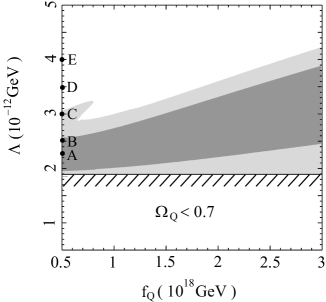
Figure 2: Constraints on the parameters $\Lambda$ and $f_{Q}$. The lightly shaded regions correspond to 99 % C.L., and the darkly shaded region corresponds to 95 % C.L. The cosmological parameters are the same as in Fig.2. The Points A $-$ E will be used as representative points in the later discussion.

Now we discuss constraints on the cosine-type quintessence models from the observations of COBE, BOOMERanG and MAXIMA. Constraints on the parameter $f_{Q}$ and $\Lambda$ are shown in Fig. 2. When we take a parameter in the oscillatory regions, the quintessence field becomes dominant component of the universe at earlier epoch. Namely the late time ISW effect becomes large and the angular diameter distance to the last scattering surface becomes smaller as mentioned before. Therefore, if $\Lambda$ is significantly large, the late time ISW effect enhances angular power spectrum at low multipoles. As a result, the heights of the acoustic peaks are suppressed relative to $C_{l}$ with small $l$.

2.2 Isocurvature Fluctuation

Next, we consider the CMB anisotropy in the case with the isocurvature mode. We calculate the CMB anisotropy for various cases, and in Table 1, we show the quadrupole $C_{2}$ normalized by $C_{10}$.

If we limit ourselves to the parameter region which is consistent with the COBE, BOOMERanG, and MAXIMA observations with simple scale-invariant primordial fluctuation, effect of the isocurvature mode is quite small as far as $r_{q}\lesssim 1$. This is because, in such cases, there is a severe upper bound on $\Lambda$ to suppress the late time ISW effect which enhances $C_{l}$ with small $l$. As a result, the quintessence field cannot dominate the universe when $z\gg 1$. Then, the isocurvature fluctuation in the quintessence density also becomes a minor effect until very recently. As one can see in Table 1, for the best-fit value of $\Lambda$ (i.e., for the Point A given in Fig. 2), the enhancement of $C_{2}$ is about 2 % even for $r_{Q}=2$. If we consider larger value of $\Lambda$, effect on $C_{2}$ is more enhanced. For $(f_{Q},\Lambda)=(5\times 10^{17}\ {\rm GeV},3.0\times 10^{-12}\ {\rm GeV})$ (i.e., for the Point C given in Fig. 3, which is allowed at 99 % C.L.), we calculate the CMB angular power spectrum and the result is given in Fig. 3. In this case, $C_{2}$ can be enhanced by the factor 2.6 if $r_{Q}=2$.

One should note that angular power spectrum of the CMB anisotropy strongly depends on the primordial spectrum of the fluctuations. Thus, the constraint on the $f_{Q}$ vs. $\Lambda$ plane is sensitive to the scale-dependence of the primordial adiabatic fluctuation which is determined by the model of the inflation. Therefore, if we adopt a possibility of a non-trivial scale dependence of the primordial fluctuation, the constraint on the $f_{Q}$ vs. $\Lambda$ plane given in the previous section may be relaxed or modified. If this is the case, larger value of $\Lambda$ may be allowed and the energy density of the quintessence field may become significant at earlier stage of the universe.

Figure 3: $C_{l}/C_{10}$ for $r_{q}=0$, 0.5, 1, 1.5, 2, 3 and 4 from below with $f_{Q}=5\times 10^{17}\ {\rm GeV}$ and $\Lambda=3.0\times 10^{-12}$ GeV.

	$r_{q}=0$	$r_{q}=0.5$	$r_{q}=1$	$r_{q}=1.5$	$r_{q}=2$
A	1.31	1.31	1.32	1.33	1.34
B	1.45	1.46	1.48	1.51	1.56
C	1.15	1.26	1.61	2.18	2.98
D	0.84	1.33	2.80	5.25	8.69
E	0.62	1.93	5.86	12.41	21.58

Table 1: $C_{2}/C_{10}$ for several values of $r_{q}$. We take $f_{Q}=5\times 10^{17}\ {\rm GeV}$, and (A) $\Lambda=2.3\times 10^{-12}$ GeV, (B) $\Lambda=2.5\times 10^{-12}$ GeV, (C) $\Lambda=3.0\times 10^{-12}$ GeV, (D) $\Lambda=3.5\times 10^{-12}$ GeV, and (E) $\Lambda=4.0\times 10^{-12}$ GeV. The Points A $-$ E are indicated in Fig. 2.

3 Conclusions and Discussion

We have studied the CMB anisotropies produced by cosine-type quintessence models. In particular, effects of the adiabatic and isocurvature fluctuations have been both discussed.

For purely adiabatic fluctuations with scale invariant spectrum, the existence of the quintessence suppresses the relative height of the first acoustic peak of the angular power spectrum compared with the $\Lambda$CDM case. This is because, in the quintessence models, the “dark energy” due to the quintessence may dominate the universe earlier than the cosmological constant case, and hence the late time ISW effect becomes more effective. As a result, the CMB anisotropy for large angular scale is more enhanced, which relatively suppresses the height of the acoustic peaks. Because of this effect, the CMB data from COBE, BOOMERanG and MAXIMA have imposed the stringent constraint on the model parameters of the quintessence models. We have also seen that the location of the the first acoustic peak shifts to lower multipole $l$ compared with $\Lambda$CDM models.

In the case of the isocurvature fluctuations, we have shown that the isocurvature fluctuations have significant effects on the CMB angular power spectrum at low multipoles in some parameter space, which may be detectable in future satellite experiments. Such effects is also seen in the tracker-type models [2]. This signal may be used to test the quitessence model, combining with the global shape of the CMB angular power spectrum.

References

- [1] M. Kawasaki, T. Moroi and T. Takahashi, Phys. Rev. D, in press (astro-ph/0105161)
- [2] M. Kawasaki, T. Moroi and T. Takahashi, astro-ph/0108081
- [3] R. R. Caldwell, R. Dave and P. J. Steinhard, Phys. Rev. Lett. 80, 1582 (1998).
- [4] Refs.[1] and [2], and references therein.
- [5] L.R. Abramo and F. Finelli, astro-ph/0101014.
- [6] C. Bennett et al., Astrophys. J. Lett. 464 (1996) L1.
- [7] P. de Bernardis et al., Nature 404 (2000) 995.
- [8] S. Hanany et al., Astrophys. J. Lett. 545 (2000) L5.
- [9] U. Seljak and M. Zaldarriaga, Astrophys. J. 469 (1996) 437.
- [10] W. Hu and N. Sugiyama, Astrophys. J. 444 (1995) 489; Astrophys. J. 471 (1996) 542.