1 Introduction

The goal of large astronomical telescopes is the concentration of large amounts of light in small areas, that is with optimum image quality. This requires that the optical configuration of the telescope be always close to an optimum state. The optimum state is defined with respect to the environment in which the telescope is operated. In space it is the diffraction image of the telescope and on the ground the image which can be obtained with a large optically perfect telescope in the presence of atmospheric disturbances, the so-called seeing disc. Deviations from this optimum state, due to wavefront aberrations generated by the optics of the telescope, are unavoidable. But, the telescope is still defined as diffraction limited or seeing limited if the degradation of the image is smaller than accepted limits. The criterion for a diffraction limited performance is that the ratio of the intensity of the real image at its center to the intensity of the diffraction image at its center, the so-called Strehl ratio, be larger than 0.8. This is achieved if the root mean square (r.m.s.) $\sigma_{{\rm w}}$ of the wavefront aberrations is less than $\lambda/14$, where $\lambda$ is the wavelength of the observed radiation. For a ground based operation, where the atmospheric effects are not corrected, the telescope can be defined as seeing limited if the equivalent ratio of the intensity at the center of the real image to the one at the center of the optimum image, the so called central intensity ratio (CIR) (Dierickx [1992]), is also greater than 0.8. Whereas, for small wavefront aberrations, the Strehl ratio depends on the square of the r.m.s. of the wavefront error, the CIR depends on the square of the r.m.s. $\sigma_{{\rm t}}$ of the slopes of the wavefront error, and also on the current seeing, expressed as the full width at half maximum $\Theta$ of the seeing disk :

$$CIR=1-2.89\bigg{(}\frac{\sigma_{{\rm t}}}{\Theta}\bigg{)}^{2}$$ (1)

$\Theta$ depends on the wavelength $\lambda$ of the light and is proportional to $\lambda^{-\frac{1}{5}}$. The goal of the design of a telescope is therefore to limit the wavefront aberrations to amounts which will guarantee a diffraction or seeing limited performance. In old passive telescopes this was attempted by using special constructional design features. With the increase in size this proved to be no longer sufficient (indeed, significant extrapolation beyond 5 m was possible neither technically nor costwise), but with the introduction of active elements, which can correct the aberrations during operation in a systematic way, the goals can nowadays be achieved also for very large telescopes. Such ground based telescopes with the goal of a seeing limited performance will be called active, those with the goal of diffraction limited performance adaptive. In space, the goal of active optics would be a diffraction limited performance. This article will only deal with active optics, which by definition does not include the correction of pointing errors, that is guiding and tracking.
Chapter 2 gives an overview of the principles of active optics. Chapter 3 introduces the relationships between the various components and parameters of an active optics system with special emphasis on telescopes with a monolithic primary mirror. Chapter 4 describes the properties and design of one type of wavefront analyser customised for an active optics system. Chapter 5 summarizes the major characteristics of the elastic modes of a meniscus mirror, which are of central importance for the control of a thin monolithic mirror, and chapter 6 deals with the theory of the support of such mirrors. Chapter 7 shows how the alignment can be controlled by active optics and chapter 8 the possibilities of changing the optical configuration and the plate scale of a telescope. Chapter 9 describes the designs of the active optics systems of the New Technology Telescope (NTT) and the Very Large Telescope (VLT) of the European Southern Observatory and chapter 10 summarizes some practical experience with these active optics systems. Chapter 11 gives a short overview of existing telescopes working with active optics and chapter 12 presents an outlook for the implementation of active optics into future telescopes with even larger mirror diameters and more than two optical components.
Most of the review deals with two mirror telescopes with altazimuth mountings and strong emphasis is put on the systems aspects. Earlier reviews have been given by Hubin and Noethe [1993] and by Wilson [1996], the latter also with a detailed presentation of the historical developments and an extensive list of references. More details about active optics with thin meniscus mirrors are given by Noethe [2000].

2 Principles of active optics

2.1 Error sources

Since the design of a telescope is strongly based on the avoidance of wavefront aberrations, we discuss first the possible error sources, shown and classified according to their frequency bandpasses, in figure 1.

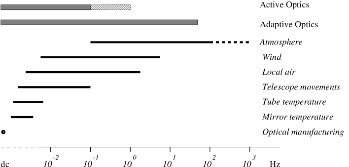
Figure 1: Bandpasses of sources of wavefront aberrations in optical telescopes

1. Optical manufacturing. These errors are constant in time. During the polishing phase the mirrors can usually not be tested together as one system. But, alone, neither of the two mirrors produces a sharp image, in particular not with an incoming spherical wavefront generated by a small pinhole. Therefore, interferometric testing is only possible with so-called null lenses which generate wavefronts which are identical to the required shapes of the mirrors. Predominantly rotationally symmetric errors in the manufacturing of these null lenses can then lead to severe errors in the shape of the mirrors in the form of spherical aberration. However, testing of null lenses is nowadays possible and, independently, the spherical aberration of the combined system can be measured in the manufacturing plant with the pentaprism test (Wetthauer and Brodhun [1920]).
2. Mirror temperature. Owing to their huge inertia and the ineffective heat exchange with the air, large telescope mirrors follow temperature variations only slowly, that is the mirrors filter out all but the lowest temporal frequencies of the air temperature variations. Nevertheless, the day to night changes of the air temperature result in temperature changes of the mirrors of possibly a few degrees. This is, unless an extremely low expansion glass is used, sufficient for a noticeable change of the focus position and other aberrations.
3. Tube temperature. Owing to its much smaller mass and therefore lower inertia, and because of a faster heat exchange due to radiative cooling, the changes of the tube temperature are much faster and larger than the ones of the primary mirror. Again, as in the case of the change of the mirror temperature, the main and possibly only significant effect is a change of the focus position.
4. Telescope movements. Any movement of the telescope tube, for example a change of the zenith angle in telescopes with an altazimuth mounting, will change to some extent the alignment of the telescope and the forces acting on the primary mirror, both effects generating wavefront aberrations. While small telescopes can be intrinsically sufficiently rigid for these effects not to play a role, large telescopes with diameters of the primary mirrors of more than, say, two meters are always noticeably affected by elastic deformations unless they are actively controlled.
5. Local air. Local air is defined here as the air inside the telescope enclosure and the air in the ground layer in the vicinity of the telescope enclosure. The local air conditions in the enclosure can be influenced by the design of the enclosure, avoidance of heat sources and active devices to maintain small temperature differences between various parts of the telescope and the ambient air (Racine, Salmon, Cowley and Sovka [1991]).
6. Wind. Wind generates both movements and elastic deformations of the telescope structure, especially of the telescope tube, as well as elastic deformations of the primary mirrors if these are sufficiently thin. Inside enclosures the peak of the energy spectrum is at approximately 2 Hz.
7. Free atmosphere. The effects of the free atmosphere above the ground layer on the image quality are predominantly generated by a layer at an altitude of approximately 10 km. The frequency range is very large, ranging from approximately 0.03 Hz to 1000 Hz.
The natural frequency for splitting the errors into two groups is the approximate lower frequency limit of the errors generated by the free atmosphere. Wavefront aberrations generated in the free atmosphere, especially at high altitude, are strongly dependent on the field angle, that is they are anisoplanatic. With integrations times larger than 30 seconds the wavefront aberrations due to the free atmosphere are effectively integrated out and the remaining aberrations are then independent of the field angle, that is, are isoplanatic. This important condition allows that the information about the wavefront aberrations obtained with a star anywhere in the field can be used to correct the images over the whole field. The lower frequency range up to the limit of 0.03 Hz includes completely the first four sources and partially the sources five to seven. Systems which systematically attempt to correct these telescope errors during operation leaving only the errors generated by the free atmosphere, and therefore to achieve a seeing limited performance will be called active optics systems, those which are predominantly designed to correct the aberrations generated by the free atmosphere and to achieve diffraction limited performance will be called adaptive optics systems. The latter work at much higher frequencies and are not the subject of this paper.

2.2 Classification of active telescopes

Up to the 1980s all telescopes were passive in the sense that after the initial setup the optical configuration was, apart from focusing, never or very rarely, and then only manually, modified. Active telescopes, on the other hand, are capable of modifying the optical configuration systematically even during operation, based on data obtained with measurements with the final, completely installed system. They can be classified according to the type of control loops and the type of correction strategies and capabilities.

2.2.1 Control loops

From a design point of view, the major differences between a passive and an active telescope are the time periods for the stability requirements of the system defining the optics on the one hand, and the role of absolute versus differential requirements on the other hand. To illustrate this point, consider first the design of a passive telescope with two mirrors. The optical configuration is fully defined by the shape of the primary mirror and the relative positions of the two mirrors. One therefore has to find support systems for both mirrors which maintain the shape and the relative positions independently of the telescope attitude for time periods of hours. The positions are mainly influenced by deformations of the telescope tube and the shape of the primary mirror by deformations of its cell. For large telescopes neither structural component can be built with sufficient stiffness since this would require deformations of the telescope tube of only a few micrometers and deformations of the primary mirror cell of less than the wavelength of light. But the variations of relative positions can be reduced by the use of Serrurier struts, which, despite the deformation of the telescope tube, make the support structures of both mirrors move in parallel when the telescope attitude is changed. The deformations of the primary mirror can be minimised by decoupling the primary mirror from the deformations of its cell by using astatic supports, which can be either mechanical levers (Lassell [1842]) or hydraulic or pneumatic devices interconnected in three groups (Yoder [1986]). All these apply forces which are independent of the distance between the mirror and its cell.
Clearly, both of these design features will only guarantee the stability of the force setting, that is the application of the correct forces for any zenith angle, and the stability of the relative positions to a certain degree. Any force errors will generate deformations of the primary mirror which are inversely proportional to its stiffness. The specifications for the tolerable wavefront aberrations will therefore define the minimum stiffness of the primary mirror and, up to diameters of approximately two meters,with the help of the scaling laws (8), (9) and (10) for thin mirrors given in §6.2, also its minimum thickness. For diameters of more than two meters, the mirrors become prohibitively thick. In addition, because of the influence of shearing forces in thick mirrors, they are more flexible than suggested by the scaling laws mentioned above. The required stiffness can therefore not be achieved by simply increasing the thickness of the mirrors. The diameters of monolithic primary mirrors of passive telescopes capable of a seeing limited or even a diffraction limited performance are consequently limited to the order of two meters.
In addition, the telescope should ideally be made of materials which do not deform under temperature variations, and, for the mirrors, guarantee a stable shape over long periods of time. The main effect of the temperature variations would be defocus, due both to a change of the length of the tube and a deformation of the mirrors. For the mirrors, the material which fulfills both requirements is low expansion glass. But, defocusing as a result of the contraction or expansion of the generally metallic structure cannot be avoided.
Active telescopes, on the other hand, do not need the stability of the forces or positions to be maintained over long periods of time. Instead, forces and positions can be changed depending on the knowledge of the passively generated deformations. This is a much easier requirement than the passive stability over time periods of hours and allows the use of less rigid elements, in particular a less rigid and therefore thinner primary mirror. The additional important question is whether these modifications are carried out in open or closed loop. Open loop changes require the knowledge and predictability of the optimum absolute forces and positions for all sky positions. A condition for this predictability is that the system be free of significant friction and therefore hysteresis effects. It should also be capable of setting these absolute forces and positions with the required accuracy over time periods of hours. On the other hand, pure closed loop operations require the stability of the forces and positions only for small time periods between two measurements of the wavefront analyser. High accuracy is then predominantly required for differential force and position settings, which can be done much more accurately than absolute settings. As a consequence, the requirements for the stability and predictability of the deformations of the optomechanical elements can, compared with open loop operations, be further reduced.
Since the number of free design parameters is much larger in active telescopes and, at least for a closed loop operation, the system also needs a wavefront analyser adapted to the mechanics of the telescopes, the design of an active telescope is more complex than the one of a passive telescope. Clearly, from the considerations above, the goal should be a closed loop active optics operation based on information from the image forming wavefront in the exit pupil. Nevertheless, open loop or mixed open and closed loop operations are also feasible. In both cases the full active optics system consists of mechanical parts performing the corrections, and wavefront sensors, which either online or offline measure the wavefront errors.

2.2.2 Correction strategy

A complete and perfect correction would, in principle, require the capability of moving all elements in all necessary degrees of freedom and correcting the shapes of all optical components. The free positioning would also enable a perfect alignment with the axis of the adapter. Such a complete correction would require measuring devices to determine the shapes and relative positions of all components. For the shapes this could be individual devices for each component and for the alignment devices for the relative orientation of two neighbouring components. In practice, a sufficient set of such devices is not always available. The alternative is to measure the combined wavefront aberrations generated by the deformations and misalignments of all components. This can be done and may only be possible by using the light from a star. The aberrations generated by the individual elements and the misalignments then have to be deduced from the total wavefront error. If this is not possible, the correction may be incomplete. On the other hand, if the errors cannot be attributed to individual elements, a correction by a subset of the elements may be sufficient, for example the correction of the deformations in a two mirror telescope with two monolithic mirrors by deformations of the primary mirror alone.
The two extreme types of active telescopes are therefore, on the one hand, those which require the control and correction of the shapes of individual components and, on the other hand, those, operating as a system, where one component can also correct errors introduced by other components.
An example of the first kind is a telescope with a segmented primary mirror with comparatively large individual rigid segments and a monolithic movable secondary mirror. The errors introduced by the primary mirror, that is the phasing and the alignment of the segments, are very different from the errors introduced by elastic deformations or the figuring of the secondary mirror and can therefore not compensate each other. As a consequence, the optical surface of both elements have to be controlled individually. An example of the latter kind is a telescope with a flexible monolithic primary mirror and also a movable monolithic secondary mirror. Here, the nature of the errors is similar and one element can correct errors introduced by the other one. The elastic and figuring errors of both mirrors are usually corrected by the primary mirror, since it is more flexible, often defined as the pupil of the telescope, and anyway equipped with a large number of supports.
The correction of errors mainly introduced by incorrect positioning of the elements, that is defocus and third order coma, has, in both types of active telescopes, to be done by appropriate movements of the optical elements.
For the type and support of flexible monolithic mirrors there are several options. On the one hand, the traditional type is a comparatively thick mirror with a force based support, which is basically passive and astatic, with an additional capability of changing the forces differentially. Such a system is ideally suited for a pure closed loop operation with time periods between consecutive corrections of the order of minutes, and, possibly with a reduced quality, also for a pure open loop operation. On the other hand, with active optics position supports also become feasible. Since these are fundamentally non-astatic they require more frequent correction and therefore, if the times between corrections are smaller than the minimum integration times for the wavefront sensing, usually a mixture of an open and a closed loop operation.
An important advantage of active telescopes is the freedom to relax the requirements for the figuring of all optical elements, since some low spatial frequency aberrations can be corrected by the active optics system. This gives the manufacturer the opportunity to concentrate on minimising the high spatial frequency aberrations. For very thin mirrors the shape of the mirror is, in a sense, only defined by the support forces. During the polishing process these cannot be controlled to the accuracy required for a perfect shape. The mirror therefore only functions together with the active optics system and its shape is only defined by that system.

2.3 Modal control concept and choice of set of modes

Most error sources generate wavefront aberrations which can be well described by certain sets of mathematical functions. Since, in many cases, a small number of these functions is sufficient to describe a wavefront aberration, a modal concept for the analysis and the correction of the wavefront errors is essential for an efficient, practical system. Which set of functions is used, depends on the dominant error sources and on the type of telescope. The choice is mainly between purely optical functions like the Zernike polynomials and vibration modes (Creedon and Lindgren [1970]) based on elastic properties of a flexible element, usually the primary mirror.
A general requirement is that the set of functions should be complete with all functions mutually orthogonal. Although only a very limited number of functions is used in practice, the completeness guarantees that, in principle, any arbitrary wavefront aberration can be well approximated. The orthogonality ensures that the values obtained for the coefficients of certain functions do not depend on other functions used in the analysis. Another important feature is the thinking in terms of Fourier modes, which means that different rotational symmetries are considered separately.
The wavefront errors generated by misalignments are defocus, third order coma and some field dependent functions, all expressible as simple polynomials. The most commonly used complete set of orthogonal polynomials over the full or annular pupil are the Zernike or annular Zernike polynomials. The errors generated by deformations of thin monolithic mirrors, on the other hand, are best described by elastic modes. These are functions with the property that the ratio of the elastic energy to the r.m.s. of the deflection is minimised. Both the Zernike polynomials and the elastic modes are also complete and orthogonal within each individual rotational symmetry.

2.4 Examples of active telescopes

Most modern large telescopes with diameters of the primary mirror of more than two meters rely in some way on active optics. The prototype of an active telescope with a system approach is the New Technology Telescope of ESO. It is a Ritchey-Chretien telescope with a meniscus primary mirror with a diameter of 3.5 m and a thickness of 241 mm. It possesses Serrurier struts and astatic mechanical levers for the support of the primary mirror. The active elements are a motorized secondary mirror with the capability to move in axial direction and to rotate around its center of curvature, and movable counterweights in the supports of the primary mirror. This allowed for a correction of defocus, third order coma and a few of the lowest order modes of the primary mirror. The principle of active optics as used in the NTT is shown in Fig. 2.
Since the telescope has still the passive design features and, for its diameter a fairly conservative thickness, corrections are only necessary every few minutes. The telescope can therefore be operated in closed loop. The additional features of its successor, the ESO Very Large Telescope (VLT), a Ritchey-Chretien telescope with a meniscus primary mirror with a diameter of 8.2 m and a thickness of 175 mm, are a motorised control of the secondary mirror in six degrees and also of the primary mirror in five degrees of freedom. Because of its much lower rigidity due to the larger diameter of eight meters and the reduced thickness of 175 mm, corrections are necessary every minute, despite the use of the usual passive design features. This correction rate still allows a pure closed loop operation.
The 10 m Keck Telescope is a Ritchey-Chretien design with a primary mirror consisting of 36 hexagonal segments, each 1.8 m across with a thickness of 75 mm and three position actuators. The telescope optics including the segments of the primary mirror is aligned approximately once per month based on data obtained from the wavefront in the exit pupil generated by a star. Afterwards the shape of the primary mirror, that is the relative positions of its segments, is maintained by an internal closed loop based on piston measurements at intersegment edges, whereas the position of the secondary mirror is controlled in open loop (Wizinowich, Mast, Nelson and DiVittorio [1994]).

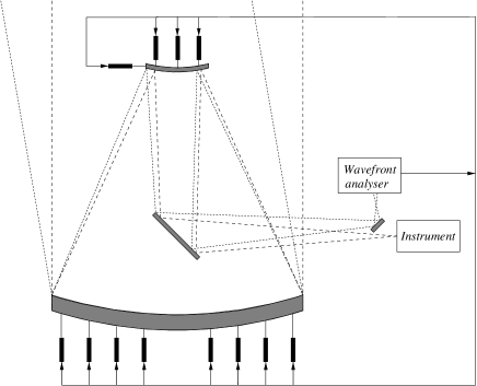
Figure 2: Principle of active optics in telescopes with a thin meniscus primary mirror

3 Relationship between active optics components and parameters

Figure 3: Dependencies between the specifications and the parameters used in an active optics design.

If the active optics corrections are done on a system level, the active optics system is not a feature added to the telescope system, but rather an integral part of it, and for many design parameters the capability to do corrections is even the driver. Fig. 3 shows for a telescope with a thin meniscus mirror the dependencies between various parameters and components of the telescope.
The column on the left contains fundamental parameters which are independent of the particular design like atmospheric effects, the safety of the mirrors under exceptional conditions like earthquakes or failures of the support systems. Also the light gathering power, defined by the diameter of the primary mirror, and the optical quality are fixed initial parameters. The optical quality is, for active telescopes, conveniently defined by two separate specifications for the high and low spatial frequency wavefront aberrations (abbreviated ’Spec. low/high SF’ in fig. 3). The parameters in the second column, that is the decision to operate in either closed or open loop and the wind speed at the primary mirror, which is determined by the design of the enclosure, can be either input parameters or the result of the system analysis. The third column contains intermediate parameters which link most of the input parameters with the parameters in the fourth column, which define the properties of the mechanical and optical components of the active optics system.
Arrows from a parameter A to another parameter B mean that B depends either directly on A, as for example the stiffness of M1 on its diameter, or that a requirement relating to B depends on A, as for example the density of supports on the number of active modes, which are the modes corrected by active optics. Lines with arrows at both ends indicate that the connected parameters can influence each other. It is then obvious from fig. 3 that limitations on mechanical parameters like the achievable accuracy of the force setting can have impacts on parameters like the allowable wind speed at M1 or the decision to operate in open or closed loop. The dependencies will be explained in detail in the following chapters. The following example will show how the diagram should be read. The required accuracy of the force setting under the primary mirror is defined by the specification for the low spatial frequency aberration and by the stiffness of the primary mirror, which determines how easily these lowest modes can be generated. The minimum stiffness itself is defined by the requirement to reduce the effects of wind pressure variations to the level given by the specification for the low spatial frequency errors of the wavefront.

4 Wavefront sensing

4.1 General considerations

In particular for telescopes which operate in closed loop, the wavefront analyser is an essential and critical part of the active optics system. In general, it is much easier to obtain the wavefront information from devices exploiting the pupil information than from measurements of the characteristics of the image. The two most widely used methods are the Shack-Hartmann method (Platt and Shack [1971]) and the curvature sensing (Roddier and Roddier [1991])). A Shack-Hartmann device, which is shown in fig. 4, measures the local tilts of the wavefront of a star somewhere in the field. A mask at the focus of the telescope prevents the light from other nearby stars entering the sensor. The telescope pupil is imaged on to an array of small lenslets, each producing in its focal plane a spot on a detector. The shift of the spot generated with light from a star compared with the position of the spot generated with a point reference source placed in the focus of the telescope is proportional to the average local tilt of the wavefront over the subaperture sampled by a single lenslet. The curvature sensing method measures the intensity variations, that is the Laplacian of the wavefront, and the shape of the edges, that is the first derivatives of the wavefront, in defocussed intrafocal and extrafocal images. Both methods work, in the end, with similar accuracy.
The wavefront sensor has to be adapted to the type of the telescope and the type of operation of the active optics system, in particular the correction strategy. One important criterion is that the measured coefficients of the modes are not dependent on the particular number of modes. This requires that the modes fitted to the measured data be orthogonal over the area of the pupil. The independence of the results for individual modes gives, for example, the freedom to correct, depending on the results, only a certain subset without the need to do another analysis with only the modes contained in this subset. Another criterion is the question whether the r.m.s. of the wavefront error or the slopes of the wavefront error should be minimised. The first choice would be the optimum for a system aiming for diffraction limited performance, the second for a system aiming for seeing limited performance. For a system working with Zernike polynomials the first choice requires a conversion of tilt data from the Shack-Hartmann device into wavefront data and a subsequent fit of the orthogonal Zernike or, for annular pupils, annular Zernike polynomials, whereas the second choice requires a direct fit of Zernike type polynomials, whose derivatives are orthogonal over the pupil, to the tilt data (Braat [1987]). A system working with elastic modes of the primary mirror has to fit functions to wavefront data, since the elastic modes, but not their derivatives, are orthogonal over the area of the mirror.
Furthermore the wavefront sensor has to fulfill a number of requirements imposed by the environment and the specification for the required accuracy, given usually in terms of tolerable low spatial frequency wavefront errors. In the rest of this section we will concentrate on the Shack-Hartmann method.

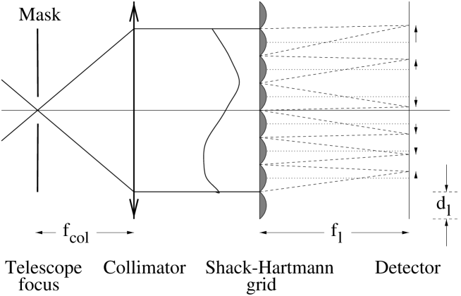
Figure 4: Shack-Hartmann optics in a telescope.

4.2 Calculation of the wavefront coefficients

The calculation of the coefficients is done in five steps.
1. Computation of local tilt values and indexing of the spots.
The centroids of the Shack-Hartmann patterns obtained with the reference and the star light are computed. A problem may be to find the reference spot corresponding to a certain star spot. One possibility would be to mark certain lenslets by reducing their transmission, another one to use the irregularities of the lenslet array to find the relative shift between the two patterns for which certain combinations of local distances give the best correlation. The second method works well for well corrected systems and grids with sufficient distortions. In practice, with highly regular grids nowadays available, the errors introduced by making a wrong correspondence are irrelevant for a first correction of strongly aberrated wavefronts. After this initial correction the pattern is so regular, that a well designed telescope with good pointing and tracking will almost always place the star spots close to the corresponding reference spots.
2. Computation of the center of the pupil.
The center of the pupil can be calculated as the simple weighted average of the positions of the reference spots of all double spots. Other more complicated algorithms may give a higher accuracy. The major goal, apart from finding the proper center of the patterns is to disregard distorted spots at the edges belonging to subapertures which are not fully inside the pupil.
3. Interpolation of tilt data to regular positions in the pupil.
In general, the Shack-Hartmann spot pattern is neither symmetric nor fixed with respect to the pupil. Each fit of a set of modes to the data involves the computation of the values of all modes at the relative locations of all spots in the pupil. The alternative is to interpolate the data to a fixed regular grid and calculate in advance the values of the modes only once for the regular grid positions in the pupil. The interpolation is done by fitting a two dimensional polynomial to the data of the surrounding spots. For a 23 by 23 pattern the optimum is the use of a second order polynomial taking into account all spots within a distance from the regular spot position of 20% of the radius of the full pattern.
4. Conversion of tilt data into wavefront data.
The conversion of a shift of a centroid $\eta_{{\rm ccd}}$ into a slope of the wavefront is given by

$$\frac{{\rm d}w}{{\rm d}\rho}=\frac{1}{2N_{{\rm tel}}\;N_{{\rm l}}}\frac{f_{{\rm col}}}{d_{{\rm l}}}\eta_{{\rm ccd}}$$ (2)

Here $w$ is the wavefront error, $\rho$ the normalised radius of the entrance pupil, $f_{{\rm col}}$ the focal length of the collimator, $d_{{\rm l}}$ the diameter, $f_{{\rm l}}$ the focal length and $N_{{\rm l}}=f_{{\rm l}}/d_{{\rm l}}$ the f-number of a lenslet, and $N_{{\rm tel}}$ the f-number of the telescope.
The tilt data are then integrated to wavefront data. This is done by integrating, for a square grid, along the $n_{{\rm rc}}$ rows and and $n_{{\rm rc}}$ columns, stopping, if necessary, at the edge of the central hole with its $n_{{\rm hole}}$ missing rows or columns, and starting a new integration at the other side. If the vector field was curl-free, for all spots the two values obtained with the integration along the corresponding column or the integration along the corresponding row, would, with a proper choice of the integration constants, be identical. But with the noise added by the measurement, this is not the case. Since the approximate number of $0.75n_{{\rm rc}}^{2}$ intersections is, for all practical grids, much larger than the number of $2(n_{{\rm rc}}+n_{{\rm hole}})$ integration constants, the optimum choice of the integration constants can be obtained with a least squares fit.
5. Fit of chosen functions to the wavefront data.
The next step is a straightforward least squares fit of the chosen set of functions to the wavefront data on the regular grid. With a fixed set of functions the fit is a multiplication with a precalculated matrix. This yields the coefficients of the fitted modes and, in addition, the residual r.m.s. $\sigma_{{\rm resid}}$ of the wavefront aberration after subtraction of the fitted modes.
6. Subtraction of field aberrations.
Since the wavefront analysis is usually done in the field of the telescope, but the active optics corrections require the coefficients at the center of the field, the contributions from the field aberrations have to be subtracted. In aligned systems these are rotationally symmetric, but in misaligned systems the patterns are more complicated as described in sec. 7. An accurate subtraction of the field effects therefore requires information on the actual misalignment of the telescope.

4.3 Definition of Shack-Hartmann parameters

The focal length $f_{{\rm col}}$ of the collimator is chosen such that the image of the pupil on the Shack-Hartmann grid and therefore also the spot pattern fits, with some margin, on the detector. This leaves then only two adjustable parameters, namely the number of lenslets sampling the pupil and the f-number of the lenslets.

• Sampling of the wavefront.
  The sampling is determined by two requirements (see fig. 3). First, it should be sufficient to guarantee an accurate measurements of the coefficients of all fitted modes. For this, the major error sources are an inaccurate determination of the center of the Shack-Hartmann pattern, the averaging of the tilts over subapertures and the aliasing generated by the finite sampling. The error due to the first source is of the order of 2.5% for a 10 by 10 sampling, with the error being approximately inversely proportional to the sampling $n_{{\rm rc}}$ in one direction. If the wavefront errors are expanded in Zernike polynomials, the latter two sources lead only to crosstalk into the next lower term in the same rotational symmetry. This crosstalk is of the order of $\delta^{2}$, where $\delta$ is the ratio of the diameter of the subaperture to the diameter of the pupil.
  Second, to guarantee for a closed loop operation a full sky coverage with field sizes of the order of 100 arcmin² available in most telescopes, the sampling should be sufficiently coarse, that is the corresponding subapertures in the pupil should be large enough to gather, with the chosen integration time, enough light from stars of magnitude 13. Measurements with two wavefront analysers in different positions in the field have shown that only with integration times of 30 seconds or more the differences due to effects of the free atmosphere at high altitude are effectively integrated out. Measurements with these integration times are therefore effectively isoplanatic and 30 seconds is the minimum time between active optics corrections in a closed loop operation. With 30 seconds integration time sufficient maximum pixel values are, at least for seeing values up to 1.5 arcsec, guaranteed with subapertures with diameters of approximately 400 mm.

• f-number of the lenslets. This parameter is determined by the requirement that a wavefront analysis can be done with high accuracy under all relevant external conditions. The major external parameter is the atmospheric seeing. The image analysis should function both under excellent seeing conditions with an expected minimum value $\Theta\approx 0.2$ arcsec and bad seeing conditions with seeing values up to at least $\Theta\approx 1.5$ arcsec. Above these values the tolerable errors, which would still guarantee a seeing limited performance, are so large that a seeing limited performance can also be achieved with open loop operations (see §10.3.3). This leads to three conditions for the f-number of the Shack-Hartmann lenslets (Noethe [2000]).
  1. Excellent seeing : Minimum spot size larger than 1.5 times the pixel size.
  For an accurate centroiding the spot diameter has to be at least 1.5 times as large as the pixel size $d_{{\rm p}}$. The minimum spot size is generated by the reference light or possibly by star light under optimum seeing conditions and is given by the diameter of the Airy disk of the lenslets. This leads to the following condition for the f-number $N_{{\rm l}}$ of the lenslets.

  $$N_{{\rm l}}\geq 1.25\frac{d_{{\rm p}}}{\mu{\rm m}}$$ (3)

  2. Bad seeing : Avoidance of swamping.
  In bad seeing conditions swamping of the spots should be avoided, i.e. the diameter of the spots due to atmospheric effects should be smaller than the diameter of the lenslets. For an assumed worst seeing of $\Theta\approx 1.5$ arcsec and a diameter of the spot less than 0.7 times the lenslet diameter one gets

  $$N_{{\rm l}}\leq 50000\frac{n_{{\rm rc}}d_{{\rm l}}}{d_{{\rm M}}}$$ (4)

  where $d_{{\rm ccd}}$ is the diameter of the CCD and $d_{{\rm M}}$ the outer diameter of the primary mirror.
  3. All seeing conditions : Maximisation of sensitivity to transverse aberration.
  The measuring accuracy of the Shack-Hartmann sensor is mainly limited by the centroiding errors. The generated wavefront error is proportional to the centroiding error with an r.m.s. $\sigma_{{\rm cen}}$, the f-number $N_{{\rm l}}$ of the lenslets and, roughly, to the square root of the number of modes used in the analysis. This leads to the condition for $N_{{\rm l}}$

  $$N_{{\rm l}}\geq 0.2\frac{\sigma_{{\rm cen}}}{\sigma_{{\rm wf},{\rm max}}}\sqrt{n_{{\rm modes}}}$$ (5)

  where $\sigma_{{\rm wf},{\rm max}}$ is the r.m.s. of the maximum tolerable wavefront error allocated to the wavefront analysis. Even with comparatively simple centroiding methods the centroiding error is of the order of only 5% of the pixel size. If the maximum pixel value is constant, the centroiding error does not depend on the spot size, but is only a function of the pixel size.

4.4 Wavefront analysers for segmented mirror telescopes

For telescopes with segmented mirrors, the wavefront analyser should be capable of detecting the deformations of individual segments, errors introduced by misalignments between mirrors, and relative tilt and piston errors of individual segments. These functions, most of them based on the Shack-Hartmann principle, have been realised in the Phasing Camera System (PCS) of the Keck telescope, which can operate in four modes (Chanan, Nelson, Mast, Wizinowich and Schaefer [1994]). The so-called passive tilt mode, where the light from each segment is collected into one spot per segment, can measure the tilt errors of the segments. The fine screen mode, where each of the 36 segments is sampled in 13 places, can measure the segment tilts, but also the defocus and decentering coma aberrations of the telescope optics, generated by a despace of the secondary mirror. Global defocus and coma introduce, over each subaperture corresponding to one segment, local defocus and astigmatism, respectively. The axial error in the position of the secondary mirror can then be calculated and corrected from the average defocus, and the tilt or decenter from the distribution of astigmatism over the subapertures. Both of these modes do not use common Shack-Hartmann lenslets, but rather a combination of prisms and a convex lens in the case of the passive tilt mode (Chanan, Mast and Nelson [1988]), and a combination of a mask, a defocusing lens and an objective with a focal length about five times smaller than the one of the defocusing lens in the case of the fine screen mode. The ultra fine screen mode samples just one segment with 217 closed packed hexagonal Shack-Hartmann lenslets.
Finally, the segment phase mode (Chanan, Troy and Ohara [2000]) deduces the relative heights of adjacent segments from the characteristic of either in-focus images or the difference between intrafocal and extrafocal images, both with star light from apertures with diameters of the order of 100 mm centered at segment edges. The in-focus method uses two algorithms. The narrowband algorithm is based on the diffraction pattern obtained with quasi-monochromatic light. The pattern is a periodic function of the relative displacement of the adjacent segments. The capture range, which is the maximum difference between the heights for which the algorithm can be applied, is of the order of 15% of the wavelength $\lambda$ of the light. For $\lambda\approx 800\,$nm the accuracy is of the order of 6 nm. The broadband algorithm takes the effects of the finite bandwidth into account. Both the capture range and the accuracy are roughly inversely proportional to the bandwidth of the light. For $\lambda\approx 800\,$nm and a bandwidth of 200 nm, the capture range is 1 $\mu$m and the accuracy 30 nm. Since both algorithms exploit interference effects, the coherence of the light over the subaperture should not significantly be degraded by atmospheric effects. This is guaranteed if the diameter of the subaperture is smaller than atmospheric coherence length $r_{0}$ for the wavelength used for the measurement. Under this condition, the results of the relative height measurements are largely independent of the current seeing. The method using the differences between the intrafocal and extrafocal images works at wavelengths of 3310 nm with a bandwidth of 63 nm. The capture range is 400 nm and the accuracy 40 nm.
Piston errors start to limit the image quality if the atmospheric coherence length $r_{0}$ for the observed wavelength $\lambda$ approaches the dimensions of the individual segments (Chanan, Troy, Dekens, Michaels, Nelson, Mast and Kirkman [1998]). Since $r_{0}$ scales with the wavelength as $\lambda^{6/5}$, phasing becomes increasingly important for observations at longer wavelengths. For segments with diameters of 1.8 m, as in the Keck telescope, phasing is effectively irrelevant for observations with visible light, but at a wavelength of 5 $\mu$m and an r.m.s. piston error of 500 nm, the central intensity is reduced by approximately 60%. At the Keck telescope the phasing tolerances are set to $\leq 100$ nm for normal observing. However, for observations also using adaptive optics to correct the atmospheric disturbances or for telescopes in space, the tolerances should be much tighter.

5 Minimum elastic energy modes

The minimum-energy modes can be defined in the following way (Noethe [1991]). Each rotational symmetry $m$ will be considered separately. Let ${\cal F}_{m,0}$ be the set of all functions of rotational symmetry $m$ defined over the area of the mirror. The lowest mode $e_{m,1}$ is the one taken from the set ${\cal F}_{m,0}$ which minimises the ratio $\Gamma$ of the total elastic energy ${\cal J}$ of the mode to the r.m.s. ${\cal A}$ of its deflection perpendicular to the surface. Let ${\cal F}_{m,1}$ be the set of all functions of ${\cal F}_{m,0}$ which are orthogonal to $e_{m,1}$. The second mode $e_{m,2}$ is the one taken from ${\cal F}_{m,1}$ which mimimizes the ratio $\Gamma$. For an arbitrary $i$ let ${\cal F}_{m,i-1}$ be the set of all functions of ${\cal F}_{m,0}$ which are orthogonal to all functions $e_{m,1},...,e_{m,i-1}$. Then, the i-th mode $e_{m,i}$ is the one taken from ${\cal F}_{m,i-1}$ which mimimizes the ratio $\Gamma$. The actual construction of the minimum-energy modes requires the solution of the variational equation

$$\delta({\cal J}-\tilde{\xi}{\cal A})=0,$$ (6)

where $\tilde{\xi}$ is a free parameter which can be interpreted as the energy per unit of the r.m.s. of the deflection. The use of variational principles leads, together with the assumptions of a thin shallow spherical shell, to a fourth order differential equation, which can be transformed into two second order differential equations for each rotational symmetry. Since the fixed points only define the position of the mirror in space and have no impact on its shape, the appropriate boundary conditions are the ones for free inner and outer edges. The solutions of the differential equations form, within each rotational symmetry $m$, a complete set $\{e\}$ of orthogonal functions, the elastic modes $e_{m,i}$. The order of a mode within each rotational symmetry is denoted by the index $i$. If the eigenvalues $\xi_{m,i}$ are expressed as

$$\xi_{m,i}=\frac{1}{2}h\gamma\omega_{m,i}^{2},$$ (7)

where $\gamma$ is the mass density of the mirror, $h$ its thickness, and $\omega_{m,i}$ is interpreted as the circular frequency of a vibration mode with the order $i$ within the rotational symmetry $m$, the differential equations are identical to the equations describing vibrations of a thin shallow shell under the assumption that in-plane inertial effects are neglected. The eigenvalues $\xi_{m,i}$, which can be shown to be proportional to the elastic energies of the modes, are therefore proportional to the square of the eigenfrequencies of the corresponding vibration modes. For geometrically similar mirrors of the same material, the eigenfrequencies scale with $h/d_{\rm M}^{2}$.

Figure 5: Left: Eigenfrequencies of the elastic modes of the VLT primary mirror for the lowest nine rotational symmetries $m$ and lowest six orders $i$ within each rotational symmetry. Right: Logarithm of the fraction $\sigma_{{\rm d}}/\sigma_{{\rm p}}$ of the deflection generated by a random pressure field left after subtraction a certain number of lowest modes.

Fig. 5 shows the eigenfrequencies of the elastic modes of the VLT primary mirror with a diameter of 8.2 m, a thickness of 175 mm and a radius of curvature of 28.8 m as a function of their order in a log-log plot. Two features of elastic modes are very useful in the context of active optics. First, the eigenfrequencies increase rapidly both with the symmetries $m$ and with the orders $i$. Within each rotational symmetry $m$ the increase in the log-log plot is approximately linear, with the symmetry 2 having the largest slope of approximately 2, that is the eigenfrequencies are roughly proportional to $i^{2}$. The lowest modes of the symmetries zero to three show, for the lowest order, deviations from the linear behaviour. For the rotational symmetries zero and one the relative increase is due to membrane stresses induced by the thin shell. In a log-log plot of the eigenfrequencies against the rotational symmetry $m$ the increases are, for $m\geq 2$, also linear, with a largest slope of approximately 2 for the lowest order one. In this order the eigenfrequencies are therefore proportional to $m^{2}$. It is obvious from the plot in fig. 5 on the left, the lowest elastic mode $e_{2,1}$ of rotational symmetry two is the by far softest and therefore most easily excitable deformation. Its control is therefore together with defocus and decentering coma, which are generated by misalignments, the most important and demanding task of active optics. Because of the fast increase of the stiffness of the modes with the order and the rotational symmetry, any given set of forces or any given pressure field will generate significant deflections only in the lowest modes. If $\sigma_{{\rm p}}$ is the r.m.s. of the deflections generated by random white noise pressure fields, figure 5 shows on the right the ratio $\sigma_{{\rm d}}/\sigma_{{\rm p}}$, where $\sigma_{{\rm d}}$ is the r.m.s. of the residual deflection after the subtraction of a given number of elastic modes with the lowest eigenfrequencies. A subtraction of the softest mode $e_{2,1}$ alone reduces the r.m.s. of the deflection to 40%, and a subtraction of the softest five modes to 10%.
Second, a pressure field, which is proportional to an elastic mode, will, since the mode is an eigenfunction of the underlying differential equation, generate a deflection with exactly the same functional dependence. The coefficient of the deflection is then inversely proportional to the eigenvalue, that is the elastic energy, of this mode. This feature can be exploited to calculate the deflections generated by arbitrary pressure fields or sets of forces. The pressure fields are directly expanded in terms of the elastic modes, whereas the forces are described as delta functions and then expanded. The total deflection is obtained by summing up the deflections in the individual modes, which are obtained by multiplying the expansion coefficients of the pressure field by factors inversely proportional to the elastic energies of the modes.

Figure 6: Lowest three eigenmodes of rotational symmetry two (dashed lines) and their corresponding annular Zernike polynomials (solid lines) as functions of the normalised radius $\rho$.

Zernike polynomials $z_{m,i}$ and elastic modes $e_{m,i}$ are very similar in the respect that, in each rotational symmetry $m$, the number of nodes of the radial function is defined by the order $i$ of the mode. For rotational symmetries larger than one the Zernike polynomials $z_{m,i}$ correspond to the elastic modes $e_{m,i}$, but for rotational symmetries zero and one, where the lowest Zernike polynomials piston and tilt represent full body motions, the elastic modes $e_{m,i}$ correspond to the Zernike polynomials $z_{m,i+1}$. The major difference between the two sets of functions is that the elastic modes are effectively linear near the outer edge but show stronger variations near the inner edge than the Zernike polynomials. The consequence is that particularly higher order elastic modes cannot be well approximated by a small number of annular Zernike polynomials. Figure 6 shows the first three annular Zernike polynomials and elastic modes of rotational symmetry two. The residual errors of fitting the elastic mode of order $i$ with $i$ annular Zernike polynomials are, in fractions of the r.m.s. of the elastic modes, 0.05 for $i=1$, 0.35 for $i=2$ and 0.62 for $i=3$. To push the residual fraction below 0.05 for the modes $i=2$ and $i=3$ one needs to fit four and six annular Zernike polynomials, respectively. Nevertheless, at least the lowest elastic modes are, in vector notation, effectively parallel to their corresponding Zernike polynomials. Examples of such pairs are Zernike defocus $z_{0,2}$ and the first elastic mode $e_{0,1}$ of rotational symmetry zero, Zernike third order coma $z_{1,2}$ and the first elastic mode $e_{1,1}$ of rotational symmetry one, and Zernike third order astigmatism $z_{2,1}$ and the first elastic mode $e_{2,1}$ of rotational symmetry two. Clearly, members of such pairs should not be fitted simultaneously to a wavefront.
The relative difference between the lowest mode $e_{2,1}$ of rotational symmetry two and the equivalent Zernike third order astigmatism ($\sqrt{6}r^{2}\cos{2\varphi}$) is only of the order of 5%. But the forces to generate third order astigmatism with an accuracy similar to the one achievable for the corresponding elastic mode $e_{2,1}$ are significantly larger. The elastic mode $e_{2,1}$ of the primary mirror of the VLT can be generated, excluding print-through effects, with an accuracy of 0.00003 with maximum forces of $F_{{\rm max}}=1.68$ N for a coefficient of 1000 nm. The accuracy, with which Zernike astigmatism can be generated, and the required forces depend on the number of elastic modes used for the approximation. With two modes the accuracy is 0.012 with $F_{{\rm max}}=4.2$ N and with six modes 0.0024 with $F_{{\rm max}}=13.6$ N. This shows again the advantage working with elastic modes rather than Zernike polynomials in the active optics corrections of elastically induced errors.
Since misalignment errors generate to first order nearly pure field independent Zernike defocus and third order coma, the Zernike polynomials $z_{0,2}$ and $z_{1,2}$ should be included and, consequently, the corresponding elastic modes $e_{0,1}$ and $e_{1,1}$ excluded from the set of fitted modes. The two Zernike modes will not exactly be orthogonal to the higher elastic modes within their rotational symmetry, but this is in practice not a significant effect. The sets of functions used in active optics then contain Zernike defocus and third order coma and, if monolithic mirrors are used, some of the elastic modes with the lowest energies. The number of elastic modes which will be considered depends mainly on the forces which are required to correct these modes. The fact that these forces increase much faster with the spatial frequencies of the modes than the coefficients of these modes generated by noise effects in the wavefront analyser, puts a natural limit on the number of modes which can be corrected. All modes which are actually corrected during the active optics process will from now on be called active modes.
The number of active modes can be defined in the following way. One can assume that the forces applied by passive actuators are accurate to approximately 5% of the nominal load over the range of usable zenith angles. Further, the r.m.s. of the wavefront error introduced by any mode should be well below the diffraction limit. Therefore, one should correct all modes which are generated with coefficients of more than, say, 15 nm by random force errors evenly distributed in a range of $\pm 5$% of the nominal load of each support. These coefficients, which will be inversely proportional to the square of the eigenfrequencies of the corresponding modes, can be calculated by the method mentioned above in this section from several runs with independent sets of random forces.

6 Support of large mirrors

6.1 System dependencies

The properties of the supports of large monolithic mirrors, in particular of the primary mirrors, of large active telescopes are related to the basic requirements in a complex way. In fig. 3 the mechanical parameters, for which requirements are to be deduced from the input parameters, are shown in the upper six boxes in the right column. Friction is the only limitation for the predictability of the system. Clearly, it also has an influence on the stability. The latter depends on the general type of the support system, the astaticities of its components and the stiffness of the primary mirror. The major safety requirement is the need to keep the stress levels, in particular at the support points, well below the critical values. These depend on the material of the mirror, and the values of the generated stress primarily on the thickness of the mirror and the type of the support system, in particular the nature of the fixed points. The generated high spatial frequency aberrations, the so-called print-through, depend clearly on the specific weight and the elasticity module of the mirror material, on the thickness of M1 and the density of supports. But it can also be influenced by the general type of the support system, for example if part of the weight of the mirror is supported by a continuous pressure field at the back surface as realised in the support of the primary mirrors of the Gemini telescopes (Stepp and Huang [1994]). The stiffness of M1, a central parameter for the active optics design, is a function of the diameter of M1, its thickness and its elasticity module. Another intermediate parameter, the number of active modes, depends, as described at the end of §5, on the stiffness of M1 and the tolerable low spatial frequency errors. The required accuracy of the force setting depends on the stiffness of M1, that is predominantly on the stiffness of the softest elastic mode $e_{2,1}$, and on the tolerated low spatial frequency aberrations, again dominated by the mode $e_{2,1}$. The range of active forces depends on the stiffnesses of the active modes, and since the accuracy of a load cell is usually inversely proportional to its range, the active range is also directly related to the accuracy of the force settings.

6.2 Scaling laws for thin monolithic mirrors

For a comparison of menisci with different diameters $d_{{\rm M}}$ and thicknesses $h$ and of their support systems with $n_{{\rm s}}$ individual supports, the following scaling laws can be used. They are given for the wavefront error $w$ and the corresponding slope errors $t$ generated by deformations of the mirror.

• Pressure field applied to the meniscus
  If the pressure fields as functions of the normalized radii of the menisci are identical, the scaling law is given by

  $$w\propto\frac{d_{{\rm M}}^{4}}{h^{3}},\hskip 14.22636ptt\propto\frac{d_{{\rm M}}^{3}}{h^{3}}$$ (8)

• Sag under the own weight
  The sag between support points under the own weight of the meniscus obeys the scaling law

  $$w\propto\frac{d_{{\rm M}}^{4}}{h^{2}n_{{\rm s}}^{2}},\hskip 14.22636ptt\propto\frac{d_{{\rm M}}^{3}}{h^{2}n_{{\rm s}}^{2}}$$ (9)

  These scaling laws can readily be derived from the ones for the pressure fields by noting that the forces applied by the own weight are proportional to the thickness $h$ of the meniscus. The factor $1/n_{{\rm s}}^{2}$ ensures that for a constant thickness the sag stays the same if the number of the supports per area, which is proportional to $d_{{\rm M}}^{2}/n_{{\rm s}}$, remains constant.

• Single discrete force
  For a single discrete differential force $\Delta F$ applied to the mirror the scaling law is given by

  $$w\propto\frac{d_{{\rm M}}^{2}}{h^{3}}\Delta F,\hskip 14.22636ptt\propto\frac{d_{{\rm M}}}{h^{3}}\Delta F$$ (10)

• Set of supports applying random force errors proportional to the nominal loads
  If a force error is proportional to the nominal load of the support, one has $\Delta F\propto d_{{\rm M}}^{2}h/n_{{\rm s}}$. Furthermore, if $n_{{\rm s}}$ supports are applying forces with random errors the expression for the effect of a single force has to be multiplied by $\sqrt{n_{{\rm s}}}$. Together one then obtains from eq. (10)

  $$w\propto\frac{d_{{\rm M}}^{4}}{h^{2}}\frac{1}{\sqrt{n_{{\rm s}}}},\hskip 14.22636ptt\propto\frac{d_{{\rm M}}^{3}}{h^{2}}\frac{1}{\sqrt{n_{{\rm s}}}}$$ (11)

The design of the support system has to meet both the specifications for the high and the low spatial frequency aberrations. The former are dominated by the sag between the support points described by the scaling law (9) and the latter by the deformation in the shape of the mode $e_{2,1}$ generated by random support forces. Since the achievable accuracy of the force setting will be proportional to the total force range, one can apply the scaling law (11), if the nominal load is understood as the force range. If, for different mirrors and their supports, the high spatial frequency errors are taken to be identical, the number of supports scales with $n_{{\rm s}}\propto d^{2}/h$ for wavefront errors and $n_{{\rm s}}\propto d^{1.5}/h$ for slope errors. The low spatial frequency errors then scale with

$$w\propto\frac{d_{{\rm M}}^{3}}{h^{1.5}},\hskip 14.22636ptt\propto\frac{d_{{\rm M}}^{2.25}}{h^{1.5}}$$ (12)

This scaling law shows that the requirements for the accuracy of the force setting increase strongly with the flexibility of the mirror. For example, if the thickness of the mirror and the density of the supports are kept constant, the required accuracy of the force setting as a fraction of the total range is inversely proportional to $d^{3}$, if the wavefront errors are to remain constant, and to $d_{2.25}$ for the slope errors.

6.3 Types of supports for thin monolithic mirrors

For thin monolithic mirrors there are three fundamental choices for the type of the support system.

1. Force or position based systems. While for passive telescopes force based systems are the only option, for active telescopes both types are feasible. The force option is currently still preferred, since it allows a certain decoupling of the mirror from the mirror cell and therefore a pure closed loop operation. For large mirrors a position based support would, owing to the fast deformations of the mirror cell, also require open loop corrections.
2. For force based systems : combination of passive and active supports or purely active supports. The combination is the best and often the only solution for a pure closed loop system, since the passive part, supporting the weight of the mirror, can be designed as an astatic system, which guarantees the required stability over sufficiently long time periods. Purely active supports usually have a level of non-astaticity which requires also open loop corrections, although possibly not as frequently as with a position based system.
3. Mechanical levers or, at least for the passive part, hydraulic or pneumatic supports. Mechanical levers add considerable additional weight and require real fixed points, which, in certain emergency cases, may have to support the full weight of the mirror. Astatic hydraulic or pneumatic systems can work with supports connected in sectors and therefore virtual fixed points. Unwanted overloads are therefore distributed over several supports. This generates, in case of failure, much smaller stresses than a support with real fixed points and is, for very flexible mirrors, the safer and therefore preferred solution.
Which of the above mentioned options is chosen depends on the maximum tolerable stress levels and the required stability of the optical configuration of the telescope system. With glass still the traditionally used, although not necessarily optimum material, the maximum stress level plays an important role. The choice of a system with real fixed points may then require a comparatively thick primary mirror, whereas a system with virtual fixed points and therefore a better distribution of the loads in exceptional circumstances may allow the use of a much thinner mirror.
In the latter case a lower limit for the thickness of the mirror is defined by the required stiffness to limit deformations by wind buffeting to values defined by the specification for the effects of wind buffeting expressed in terms of low spatial frequency aberrations. This can be partially ameliorated by coupling the mirror for high temporal frequencies to its, in general, stiffer mirror cell, for example by using a mirror support with six fixed points as described in §6.4.3 (Stepp [1993]).
To be able to remove the mirror easily, for example for realuminisation, from its cell, it would be an advantage to have only push supports. While this is not possible for the optimum solutions for the lateral supports presented in §6.5, it can be realised for the axial supports. The only restriction will be a limitation for the maximum zenith angle $\theta_{{\rm z,max}}$ for which the telescope optics can be corrected with the active optics system. The reason is that the largest required negative correction force $F_{{\rm corr}}$ has to be smaller than the remaining gravity load which varies with the cosine of the zenith angle. If $F_{{\rm G},0}$ is the nominal gravity load at zenith angle zero, one gets $\theta_{{\rm z,max}}=\arccos(F_{{\rm corr}}/F_{{\rm G},0})$. For larger zenith angles than $\theta_{{\rm z,max}}$ the mirror would, at a given support point, loose the contact with the support. One goal of the active optics design should therefore also be to minimise the required range of the active forces.

6.4 Axial support of thin meniscus mirrors

6.4.1 Basic support geometry

For the distribution of the axial supports one can choose between two basic geometries. One would be a regular geometry with hexagonal symmetry where neighbouring supports form equal lateral triangles. This would be the most effective solution in terms of the required number of supports, but the symmetry is not compatible with the circular shape of the mirror. The other choice are discrete supports on circular rings. Over most of the area the support geometry is then irregular, but near the edges the deformations are more regular than those generated by the hexagonal support. The usual choice is the second option, also because analytical methods are available at least for the optimisation of the ring radii.

6.4.2 Minimisation of wavefront aberrations

The theory for the analytical optimisation of the radii of the support rings for thin plates has been developed by Couder [1931] and the one for thin shallow shells by Schwesinger [1988]. Both calculate first the deflections for a support on a single continuous concentric ring. The total deflection is then a superposition of the deflections generated by $n$ rings, multiplied by the appropriate load fractions. Since the dependences of the deflections on the radii are not linear, optimisations can only be done by trial and error methods. The final result of the optimisation depends also on two other parameters which are, in addition to the radii, considered variable, namely the load fractions and, introduced by Schwesinger [1988], an overall deformation in form of a paraboloid, which can easily be corrected by an axial movement of the secondary mirror. Compared with the results which are obtained under the condition that all support forces are identical, that is that the load fractions are fixed and no defocus is allowed, the r.m.s. of the sag between the supports can be reduced by approximately 30% if the additional degrees of freedom of the load fractions and, more important, the defocus are used for the optimisation. The reason for the strong effect of the defocus component is that the deflections near the inner and outer edges are nearly linear and, if the support forces generate an overall shape similar to a parabola, a fitted parabola can intersect the deflection curve twice both between the inner edge and the inner ring and the outer edge and the outer ring.

6.4.3 Effects of fixed points

Any basically astatic axial system needs three fixed points for the definition of the position of the mirror in space. These can be either real, as in the case of astatic mechanical lever supports, or virtual, as in the case of hydraulic or pneumatic supports, where all supports in each of three sectors are interconnected. Since the volume of the fluid or gas is constant in each sector, the barycenter of the supports will stay constant. If the positions of the virtual fixed points are defined as these barycenters, the two types of fixed points can mathematically be treated in the same way. In the case of the real fixed points, they usually replace, on one of the rings, three of the astatic or active supports at angular separations of $120^{\circ}$.
The question now arises, whether modes of a given rotational symmetry $m$ can be corrected with a given number of supports $n_{{\rm s}}$ on one ring without exciting appreciable deformations in other rotational symmetries. Let us assume that the force changes at the actuators on one ring follow the rotational symmetry $m$. The reaction forces on the fixed points due to changes of the actuator forces can easily be calculated from the conditions of the equilibrium of the forces and the two moments around two orthogonal axes perpendicular to the axis of the mirror. It can then be shown (Noethe [2000]) that the sums of the applied forces and the reaction forces on each support on the ring do not follow the rotational symmetry $m$ any more, if the rotational symmetries of the applied forces are zero, one, $n_{{\rm s}}-1$, $n_{{\rm s}}$ or $n_{{\rm s}}+1$. For the rotational symmetries zero and one the reaction forces can be made zero, if more than one ring is used and, in addition, for $m=0$, the sum of load fractions on the rings is zero or, for $m=1$, the sum of the products of the load fractions and the corresponding ring radii, is zero. The largest rotational symmetry correctable with the axial support system is then $n_{{\rm s}}-2$, where $n_{{\rm s}}-2$ is the smallest number of supports on any of the rings.
Another effect of the fixed points is that the correction of modes with all symmetries different from multiples of three lead to additional tilt. The coefficient of the tilt is roughly equal to the coefficient of the corrected mode. In practice, it is very small and anyway quickly removed by the autoguider.
An interesting consideration, first suggested by the Gemini project (Stepp [1993]), is the use of six fixed points to couple the mirror to the, in general, stiffer mirror cell. This allows the reduction of wind buffeting effects on the primary mirror. Of course, the mirror should be coupled to its cell only for high temporal frequencies. For low temporal frequencies it has to be decoupled to facilitate active optics corrections and, if intended by the design, to guarantee a basically astatic support. This can be achieved by splitting each of the three sectors in a hydraulic support system with interconnected supports into two smaller sectors and connecting the halves by a tunable valve. A straightforward calculation (Noethe [2000])) shows that only modes with rotational symmetries

$$m=\;6i-1\;\;{\rm or}\;\;m=\;6i\;\;{\rm or}\;\;m=\;6i+1,\;\;\;\;\;\;\;i=0,1,2,...$$ (13)

are compatible with a six sector support, that is, are decoupled from the mirror cell. For all other rotational symmetries, in particular the rotational symmetry two with the softest and therefore most easily excitable first mode, the mirror is coupled to the cell and deformations in form of these modes can therefore be reduced.

6.4.4 Effect of support geometry on mode correction

Not only the fixed point reactions, but also the number of supports alone on any of the rings limits the correctability of certain modes. Let $m$ be the rotational symmetry followed by the active forces on one support ring, $\theta$ the offset angle, $n_{{\rm s}}$ the number of supports on the ring, and the set S be defined by ${\bf S}=\{p\,:\,p=j\cdot n_{{\rm s}},j=0,1,2,...\}$. The wavefront aberration generated in an arbitrary rotational symmetry $\overline{m}$ and order $j$ is given by (Noethe [2000]) :

$$w_{\overline{m}}(\varphi)\propto\left\{\begin{array}[]{ll}\cos{\overline{m}\varphi}\;\cos{m\theta},&m+\overline{m}\in{\bf S}\;\;{\rm and}\;\;m-\overline{m}\in{\bf S}\\ \cos{(\overline{m}\varphi-m\theta)},&m+\overline{m}\in{\bf S}\;\;{\rm and}\;\;m-\overline{m}\in/\hskip 4.2679pt{\bf S}\\ \cos{(\overline{m}\varphi+m\theta)},&m+\overline{m}\in/\hskip 4.2679pt{\bf S}\;\;{\rm and}\;\;m-\overline{m}\in{\bf S}\\ 0,&m+\overline{m}\in/\hskip 4.2679pt{\bf S}\;\;{\rm and}\;\;m-\overline{m}\in/\hskip 4.2679pt{\bf S}\end{array}\right\}$$ (14)

The first three cases represent the combinations of the rotational symmetry $m$ of the forces and the number $n_{\rm s}$ of the equidistant supports on one ring which generate crosstalk into other rotational symmetries $\overline{m}$. For example, a force pattern with a rotational symmetry $m=4$ on a ring with $n_{{\rm s}}=9$ supports will generate the required wavefront deformation $w_{4j}(r)\cos{4\varphi}$, but also an unwanted crosstalk of the form $w_{5j}(r)\cos{5\varphi}$. The same two wavefront aberrations are generated by a force pattern with the same maximum force but with a rotational symmetry $m=5$, since the forces with rotational symmetries $m_{1}$ and $m_{2}$ on a ring with $m_{1}+m_{2}$ supports are identical. Most significant are couplings into the mode $e_{0,2}$. A support with, say, nine supports on one of the rings will generate crosstalk into this mode if a mode with the symmetry seven is corrected.

6.5 Lateral support of thin meniscus mirrors

Lateral support systems are usually passive and should fulfill the following two requirements. First, they should not, for any inclination of the mirror, generate wavefront aberrations which require significant active correction forces from the axial support system, which would increase the range of active forces and therefore reduce the maximum usable zenith angle as described at the end of §6.3. Second, the mirror should be supported at the outer edge only. Fortunately, a type of lateral support with these characteristics exists. The analytical theory has been developed by Schwesinger [1988, 1991]. Instead of discrete forces it considers initially force densities at the edges with the three components $f_{{\rm r}}$ in radial, $f_{{\rm t}}$ in tangential and $f_{{\rm a}}$ in axial direction. Thinking in Fourier terms implies that any force densities which follow a given rotational symmetry generate deformations in only this symmetry. The only force densities which support the weight of the mirror are those with the rotational symmetry one. A lateral support system should therefore only contain force densities of rotational symmetry one.
The lateral support is greatly simplified for telescopes with altazimuth mountings. In this case the directions of the forces with respect to a coordinate system which is fixed to the mirror are constant. Only the moduli depend on the inclination of the mirror cell.
If the mirror is neither too steep nor too thin, it can be laterally supported at the outer rim under its center of gravity. But for steep and thin mirrors this is not the case and axial forces at the outer edge have to be used to balance the moment. The modulus of the axial force density $f_{{\rm a}}$, which is proportional to $\sin{\varphi}$, where $\varphi$ is the azimuth angle starting from the direction parallel to the altitude axis, is then defined by the weight of the mirror, its diameter and the distance between the plane of the supports and the center of gravity of the mirror. The radial force densities $f_{{\rm r}}$ have always to be proportional to $\sin{\varphi}$ and the tangential force densities $f_{{\rm r}}$ to $\cos{\varphi}$. The only free parameter is then the fraction $\beta$ of the weight supported by the tangential force density, with the remaining weight $1-\beta$ supported by the radial force density.
Schwesinger [1988, 1991] has derived analytical formulae for the dependence of the radial function of the deflection with the rotational symmetry one on the ratio $\beta$. The deflection may contain third order coma, which can be corrected by a movement of the secondary mirror. The residual wavefront error after fitting and subtracting third order coma should therefore be the merit function for the optimisation with the ratio $\beta$. These wavefront errors are, for an optimum choice of $\beta$, in practice so small that a possible further reduction with additional supports at the inner edge is not necessary (Schwesinger [1994]).
Schwesinger’s theory for the rotational symmetry one can be extended to all other rotational symmetries (Noethe [2000]). The deformation of the mirror in any rotational symmetry $m$ can be calculated for force densities $f_{{\rm r}}$, $f_{{\rm t}}$ and $f_{{\rm a}}$ following the same symmetry $m$. Each of the three components in radial, tangential and axial direction of any of the discrete forces at the edge can then be expanded in an infinite series in all rotational symmetries. Since, as in the case of the elastic modes for axial deformations, the deflections decrease rapidly with the rotational symmetry of the modes, the consideration of the lowest symmetries will be sufficient to calculate the overall deformations. This offers a fast and efficient alternative to finite element calculations.
If the lateral supports are combined with the axial supports as in the Subaru telescope (Iye [1991]), the actual locations of the application of the forces have to be in the neutral surface to avoid unwanted moments. For solid monolithic mirrors this requires the drilling of additional holes. For mirrors with a honeycomb structure it may be the natural and best solution.

6.6 Segmented mirrors

Although it is not a compulsary requirement, one goal of a segmented mirror design is that the shapes of individual segments do not need active corrections during the operation of the telescope. With diameters as large as 2 m they require passive, astatic supports as, for example, multi-stage whiffle trees which apply both axial and lateral forces. The deflections as functions of the number of supports per segment area and thickness follow the scaling laws for monolithic mirrors given in §6.2. An optimisation of the distribution of supports is usually done with finite element calculations. To correct figuring errors in a d.c. mode, static devices like warping harnesses can be installed at the back surface of the segments.
If each segment is intrinsically stable, the major problem is the alignment of the $n_{{\rm s}}$ segments both in piston and tilt. Each segment therefore needs three actuators capable of changing the axial positions of the three fixed points. The support of a segmented mirror as a whole is therefore position based and requires, owing to the normally strong flexure of the cell with a change of the zenith angle, frequent corrections. The alignment and control of a segmented mirror is dicussed in §7.2.

7 Alignment

7.1 Alignment of a two mirror telescope

In a perfectly aligned two mirror telescope the axes of the primary mirror, the secondary mirror and the rotator are congruent. This ideal case can, in particular with large telescopes, only be achieved as an approximation. In particular, even if the alignment is sufficiently good for a certain zenith angle, the mechanical deformations of the telescope structure may generate misalignments at other zenith angles. A complete alignment of the telecope can be done in three steps.

• Initial alignment with auxiliary equipment
  Using autocollimation and finite focusing the axes of M2 and the rotator of a large telescope like the VLT can be aligned to an accuracy of approximately 3 arcsec for the angles between the axes and less than 1 mm for a shift of the vertex of M2 with respect to the axis of the rotator. But the position of M1 and therefore the angle between the axes of M1 and M2 and the shift between the vertex of M2 with respect to the axis of M1 are only defined within the mechanical tolerances of the M1 support, which are much larger than the accuracy of the alignment achieved for the relative alignment of the axes of the rotator and M2. The consequence will, in general, be a large amount of decentering coma.

• Correction of decentering coma
  The decentering coma generated by the misalignment between the axes of M1 and M2 can be measured by the wavefront analyser, and be corrected by a rotation of the secondary mirror around its center of curvature, by a full body movement of M1, or by a combination of both. After this operation the telescope may still be a schiefspiegler (WILSON [1996]) in which the axes of M1 and M2 are not aligned, but intersect at the so-called coma free point. This is a point around which the secondary mirror can be rotated without changing the value of field independent decentering coma.

• Alignment of the axes of M1 and M2
  The residual misalignment can be determined from a mapping of the pattern of third order astigmatism, that is from measurements of this coefficient at a few field positions. A complete correction can be done by rotating either the secondary mirror or the primary mirror or both around the coma free point.

An overview of aberrations in misaligned telescopes can be found in Wilson [1996] and of the alignment of telescopes in chapter 2 of Wilson [1999]. A general theory of low order field aberrations of decentered optical systems has been given by Shack and Thompson [1980]. In particular it has been shown that the general field dependence of third order astigmatism can be described by a binodal pattern, known as ovals of Cassini. Only for special cases such as a centered system do the two nodes coincide and the field dependence reduces to the well known rotationally symmetric pattern with a quadratic dependence on the distance to the field center. These general geometrical properties have been used by McLeod [1996], starting from equations by Schroeder [1987], for the alignment of an aplanatic two mirror telescope. McLeod showed that the components $Z_{4}$ and $Z_{5}$ of third order astigmatism of a two mirror telescope with the stop at the primary mirror for a field angle $\theta$ with components $\theta_{x}$ and $\theta_{y}$ are given by

$$Z_{4} = B_{0}\,(\theta_{x}^{2}-\theta_{y}^{2})\,+\,B_{1}(\theta_{x}\alpha_{x}\,-\,\theta_{y}\alpha_{y})$$ (15)

$$+\,B_{2}\,(\alpha_{x}^{2}-\alpha_{y}^{2})$$

$$Z_{5} = 2B_{0}\,\theta_{x}\theta_{y}\,+\,B_{1}(\theta_{x}\alpha_{y}\,+\,\theta_{y}\alpha_{x})\,+\,2B_{2}\,\alpha_{x}\alpha_{y}$$ (16)

$B_{0}$ is the coefficient of field astigmatism for a centered telescope, whereas $B_{1}$ and $B_{2}$ only appear in decentered systems. Numerical values for $B_{0}$, $B_{1}$ and $B_{2}$ were obtained by using general formulae for field astigmatism of individual mirrors and adding the effects of the two mirrors. The values for $\alpha_{x}$ and $\alpha_{y}$ could then be obtained from measurements of $Z_{4}$ and $Z_{5}$ in the field of the telescope.
Explicit expressions for the third order astigmatism parameters $B_{0}$, $B_{1}$ and $B_{2}$ as functions of fundamental design parameters and optical properties of the total telescope and of the position of the stop along the optical axis give more insight into the characteristics of field aberrations of two mirror telescopes. They have been derived for centered two mirror telescopes by Wilson [1996] and for decentered ones by Noethe and Guisard [2000]. In a decentered system one also has to take into account the definition of the field center. The normal definition is the direction parallel to the axis of M1, projected towards the sky. But in decentered system the image of an object in this field center is not in the center of the adapter, where the instruments are located and which is therefore the practical field center. If the field astigmatism is calculated with respect to this practical field center, the structure of the Eqs. (15) and (16) remains the same, but the parameters $B_{0}$, $B_{1}$ and $B_{2}$ change and $\theta$ denotes the field angle with respect to the center of the adapter (Noethe and Guisard [2000]). To align the axes of the two mirrors and to put the intersection of this axis with the focal plane to the center of the adapter, one has to reposition both mirrors.
In principle, two wavefront analysers would be necessary and also sufficient for a closed loop alignment of a two mirror telescope. With only one wavefront analyser available, mappings have to be done at various zenith angles and the alignment can be controlled only in open loop.

7.2 Alignment of a segmented mirror

The alignment procedure described in this section is the one used in the Keck telescope. It is assumed that the shapes of the segments are not affected by changes of the zenith angle. The control of the position of a segment is restricted to three degrees of freedom, a piston coordinate parallel to the optical axis of the telescope, and two tilt components for rotations around two orthogonal axes perpendicular to the optical axis. The alignment of the segments is done in two steps.
First, the tilts of the $n_{{\rm s}}$ segments are measured optically with the passive tilt or the fine screen mode of the phasing camera system (PCS) described in §4.4. The required corrections of the segment tilts are done by appropriate differential movements of the $3n_{{\rm s}}$ piston actuators. Second, the differences in height at midpoints of intersegment edges are measured optically by the segment phase mode of the PCS. The number of these sampling points is larger than the number of degrees of freedom, which is equal to the number of segments minus one. The optimum differential piston movements, which are the ones that minimise the r.m.s. of the differences in height of adjacent segment midpoints, are obtained by a least squares fit.
The relative positions of the segments, and therefore the overall shape of the mirror, are then maintained by the positions actuators, but not in closed loop controlled by optical measurements with the PCS, but by measurements with position sensors located at intersegment boundaries. These piston sensors are capable of measuring changes in the relative heights of the adjacent segments perpendicular to the surfaces. The actual readings after an alignment described above are defined as target values for subsequent corrections. The number of the piston sensors must be at least as large, but is usually larger than the number of actuators, which is $3n_{{\rm s}}$. The differences between the reference and the actual readings are, via a least squares fit, converted into actuator movements. Any noise in the sensor readings will lead to errors in the relative tilt and piston values of the segments. These aberrations can conveniently be expanded in so-called normal modes (Troy, Chanan, Sirko and Leffert [1998]). Similar to the elastic modes, which are eigenvectors of a differential equation decribing the elastic behaviour of the mirror, the normal modes are orthogonal eigenvectors associated with a singular value decomposition of the control matrix connecting actuator movements to the larger number of sensor readings. Apart from the discontinuities due to the segmentation, the normal modes, in particular the lower order ones, approximate to Zernike polynomials.
If random noise is assumed for the sensor readings, the average of the coefficient of a normal mode contained in the wavefront error decreases rapidly with the order of the mode. The normal mode which can most easily be generated by the segmented primary mirror control system of the Keck telescope is a defocus mode, followed by a mode similar to third order astigmatism. The defocus mode is produced by a constant offset to all piston sensors, since the corresponding changes of the actuator lengths will exactly follow a parabola. Compared with the equivalent case of the average content of modes in a wavefront generated by random pressure fields on a monolithic mirror, the decrease is, above all for the higher order modes, much weaker. For example, the normal mode similar to the third order Zernike polynomial of rotational symmetry two, that is seventh order astigmatism, is only ten times weaker than the strongest mode, whereas the corresponding ratio for the elastic modes is of the order of 200 times weaker. This slower convergence is of importance, since the higher order modes generate stronger edge discontinuities. On the other hand, the r.m.s. of the edge discontinuities related to tilt errors with a given r.m.s. value are much smaller than expected from a random distribution of the tilt errors over the segment, since most of the tilt error is contained in the smooth modes with small edge discontinuities.

8 Modification of the telescope optical configuration

A defocus aberration can be introduced both by an axial movement of the secondary mirror and a deformation of the primary mirror. This feature can be used to control the plate scale of the telescope. The defocusing with the secondary mirror can also, together with an elastic deformation of the primary mirror, be used to maintain the optical quality of the telescope during a change of its optical configuration.

8.1 Control of the plate scale

The focal length $f^{\prime}_{2}$ of M2 is assumed to be constant. The plate scale is therefore only affected by changes of the focal length $f^{\prime}_{1}$ of M1 and the distance $d_{1}$ between M1 and M2. A change of the shape of the primary mirror in the defocus mode, described by the coefficient $c_{{\rm def}}$ of the equivalent wavefront change, generates the following change $\delta f^{\prime}_{1}$ of the focal length of M1

$$\delta f^{\prime}_{1}=8\,N_{1}^{2}\,c_{{\rm def}},$$ (17)

where $N_{1}$ is the f-number of the primary mirror. The dependences of the variations of the back focal distance $b$ and the focal length $f^{\prime}$ on the variations of $f^{\prime}_{1}$ and $d_{1}$ are given by Wilson [1996]

$$\delta b = (m_{2}^{2}+1)\,\delta d_{1}-m_{2}^{2}\,\delta f^{\prime}_{1}$$ (18)

$$\delta f^{\prime} = \frac{m_{2}^{2}}{f^{\prime}_{2}}\;(f^{\prime}_{1}\,\delta d_{1}-(f^{\prime}_{2}+d_{1})\,\delta f^{\prime}_{1}),$$ (19)

where $m_{2}$ is the magnification of the secondary mirror.
The two conditions for a control of the plate scale in the telescope are the amount of the change $\delta f^{\prime}$ of the focal length of the telescope and the requirement that the distance $b$ between the pole of M1 and the image remains unchanged, i.e. $\delta b=0$. These two conditions can be fulfilled by variations of the two parameters $f^{\prime}_{1}$ and $d_{1}$.
From (18) one then gets

$$\delta f^{\prime}_{1}=\frac{m_{2}^{2}+1}{m_{2}^{2}}\delta d_{1}$$ (20)

Introducing this into (19) and solving for $\delta d_{1}$ one gets

$$\delta d_{1}=\frac{1}{m_{2}^{2}-1-\frac{d_{1}}{f^{\prime}_{2}}}\delta f^{\prime}$$ (21)

The accuracy of the control of the plate scale is limited by the accuracy of the force setting under M1 and the axial positioning of M2, that is by the individual contributions from $\delta d_{1}$ and $\delta c_{{\rm def}}$ to $\delta f^{\prime}$, and by the noise in the wavefront measurements.

8.2 Modification of the optical configuration

If a two mirror telescope has both Nasmyth and Cassegrain foci, it may not be possible to find a convenient design which places both foci at the same distance from the secondary mirror. Switching from one focus to the other therefore requires refocusing. In a classical Cassegrain design this will generate field independent third order spherical aberration, which was initially not present, and in a Ritchey-Chretien design in addition field dependent third order coma. Of those, the spherical aberration can be removed by a deformation of the primary mirror, that is a change of its conic constant.
Changing the shape of M1 by a function proportional to $r^{4}$ requires comparatively strong forces, since $r^{4}$ has strong curvature near the outer edge contrary to elastic modes with effectively no curvature near the outer edge. The curvature of $r^{4}$ near the outer edge can be greatly reduced by adding an appropriate amount of defocus which will be compensated by an additional axial movement of M2. This new deformation can be better approximated by elastic modes and can therefore be generated with much smaller forces.

9 Active optics design for the NTT, the VLT and the Keck telescope

9.1 General requirements and specifications

The NTT and VLT are examples of active two mirror telescopes with monolithic meniscus mirrors. The NTT with a mechanical diameter of its primary mirror of 3.58 m was the first telescope with active optics as an integral part of its design. Nevertheless, since it was the first attempt to build an active telescope, one conservative requirement was that it could, with a reduced optical quality, also function in a fully passive mode. The VLT with a diameter of its primary mirror of 8.2 m was envisaged to function only in the active mode, since its primary mirror is about 40 times as flexible. The designs of the active optics systems of these two telescopes can serve as typical examples for two mirror telescopes of the four and eight meter class with monolithic primary mirrors.
The specifications for the NTT were given in terms of the diameter $d_{80}$ of the circle containing 80% of the geometrical energy. For a Gaussian point spread function one has $d_{80}\approx 1.5\theta\approx 2.54\sigma_{t}$ and for an atmospheric-seeing point spread function $d_{80}\approx 1.9\theta$. The specifications were then $d_{80}=0.15$ arcsec for the active and $d_{80}=0.40$ arcsec for the passive mode. The figure for the active mode can be split into $d_{80}=0.10$ arcsec for the high and also $d_{80}=0.10$ arcsec for the low spatial frequency aberrations. The specifications for the VLT were given in terms of the central intensity ratio $CIR$, namely $CIR=0.8$ for a seeing of 0.4 arcsec. The relevant contributions for the design of the active optics system were $CIR=0.992$ or, according to eq. (1), an r.m.s. of the wavefront slopes $\sigma_{{\rm t}}=0.021$ arcsec for the high spatial frequencies of M1, $CIR=0.979$ or $\sigma_{{\rm t}}=0.034$ arcsec for the active optics control errors of the wavefront, including both the wavefront analysis and the corrections, and $CIR=0.97$ or $\sigma_{{\rm t}}=0.041$ arcsec for the effects of wind pressure variations on M1. Since the major aberrations generated by wind and active optics control errors are low spatial frequency aberrations, the $CIR$ figures for these error sources can be converted into approximate r.m.s. values $\sigma_{{\rm w}}$ of wavefront aberrations dominated by the mode $e_{2,1}$. $CIR=0.99$ is then equivalent to $\sigma_{{\rm w}}=140$ nm and $CIR=0.98$ to $\sigma_{{\rm w}}=200$ nm. Finally, all possibly occurring stresses in the mirrors had to be well below the critical values for glass ceramics.
With these specifications all parameters in the first column of fig. 3, which form the basis of the active optics design, were defined. Two other parameters, which are in principle free in fig. 3, were also defined in advance. First, the active optics systems of both telescopes were required to work fully in closed loop with integration times of the wavefront analyser of at least 30 seconds and a full sky coverage, and, second, the substrate of both primary mirrors was a glass ceramic.
The VLT had the additional requirement that it should work both with the Nasmyth foci and a Cassegrain focus with the consequences described in §8.2. Furthermore, because of the strong impact of temperature differences between the mirrors, the air in the enclosure and the outside air on the image quality, the VLT was required to control these differences within narrow limits instead of relying on natural ventilation only as in the case of the NTT.
The specifications for the Keck telescope were given in terms of $d_{80}$. The error budget for the total telescope was 0.41 arcsec, with 0.24 arcsec for the segment figure being the largest contribution. The total active optics error budget was split into a contribution of 0.084 arcsec from zenith distance independent and of 0.058 arsec from zenith distance dependent errors (Cohen, Mast and Nelson [1994]).

9.2 Active optics design of the NTT

9.2.1 Thickness of M1, type of support system and set of active modes

The main driver for the thickness of M1 was the requirement, that the telescope could, although with a reduced optical quality, be operated also in a passive mode. Measurements at the equatorially mounted ESO 3.6 m telescope showed that the $d_{80}$ values due to low spatial frequency elastic aberrations were of the order of 0.5 arcsec largely independent of the sky position (Wilson [1999]). Since the design of the M1 support of a telescope with an altazimuth mounting like the NTT was significantly easier, it was estimated that the NTT could, passively, achieve the same performance with a mirror of approximately half the thickness, which was then finally defined as 241 mm. Another way of justifying this thickness of M1 is the following. The average coefficient of the dominant low spatial frequency mode $e_{2,1}$ generated with random forces in the range of $\pm 1$ N would be 5.5 nm, with maximum values of the order of 15 nm. Random force errors in the range of $\pm 5\%$ of the nominal forces of approximately 760 N would then generate on average coefficients of $e_{2,1}$ of the order of 210 nm, which is equivalent to an r.m.s. of the slope errors of $\sigma_{{\rm t}}\approx 0.082$ arcsec and $d_{80}\approx 0.20$ arcsec. If equal tolerances were also given to the defocus and decentering coma errors, one would with a quadratic sum just fulfill the specification for $d_{80}=0.4$ arcsec for the passive mode.
With such a thickness the stresses, which arise if the mirror is unintentionally supported by three points only, are well below the tolerable limit. This then allowed the use of a conventional support with astatic levers and consequently three real fixed points. To define the set of active modes, one can apply the procedure described at the end of §5. With the r.m.s. of 210 nm for the average coefficient of $e_{2,1}$ generated with random forces in the range $\pm 5\%$ of the nominal load, the frequency limit for the modes to be considered is $\nu_{2,1}\sqrt{210/15}\approx 430$ Hz and the data in table 1 show that for the NTT the modes up to $e_{4,1}$ should be corrected. But then, since the elastic mode $e_{0,1}$ is replaced by defocus, there would be no possibility to correct rotationally symmetric aberrations other than defocus. Because of the importance of spherical aberration the elastic mode $e_{0,2}$ has to be added to the set of active modes. The chosen force range of the active actuators of $\pm 30$% of the nominal load was large enough to allow also the use of the equivalent Zernike modes instead of the more efficient elastic modes. Spherical aberration can be generated with much smaller forces by combining it with a defocus deformation of M1. This defocus can then easily be compensated by an appropriate axial movement of M2. For the NTT the best combination is $r^{4}-3.6r^{2}$.

Table 1: Eigenfrequencies of the lowest elastic modes of the NTT and the VLT.

Symmetry	2	3	0	4	1	5	2	0	6
Order	1	1	1	1	1	1	2	2	1
NTT	115	273	192	479	434	732	737	852	1034
VLT	16	38	42	66	68	102	107	119	143
Symmetry	3	1	7	4	8	2	0	5	3
Order	2	2	1	2	1	3	3	2	3
NTT	1131	1229	1383	1577	1779	1749	2050	2077	2366
VLT	160	176	192	221	246	246	272	289	331

9.2.2 Axial support of M1

The axial support of the primary mirror of the NTT consists of four rings with 9, 15, 24 and 30 supports. This distribution gives an r.m.s. $\sigma_{{\rm w}}$ of the high spatial frequency wavefront aberrations of approximately 7 nm and an r.m.s. of the slope error of the wavefront of $\sigma_{{\rm t}}\approx 0.02$ arcsec, well below the specification of $\sigma_{{\rm t}}=0.04$ arcsec, which is equivalent to $d_{80}=0.1$ arcsec. The chosen density of supports was also sufficient to generate all active modes with high accuracy. The largest error in terms of the r.m.s. of the relative difference between the requested and the actually generated shapes is, not considering the effects of the print-through, of the order of only 2% for the second mode $e_{0,2}$ of rotational symmetry zero. For the other modes the relative errors are of the order of 0.1% or smaller.
The modification with respect to a passive support with astatic mechanical levers were motorised counterweights which could change the support force by approximately $\pm 30$% of the gravity load on the support. Since the gravity loads are proportional to the cosine of the zenith angle, the correction of errors which are independent of the zenith angle like polishing errors would have required different positions of the counterweights for different zenith angles. For this reason additional springs were introduced which could introduce correction forces independently of the zenith angle. The springs had no motorised control and could only be adjusted manually.
With the comparatively large thickness, wind buffeting on M1 was no problem. In addition, the telescope optics was very stable over time periods of one minute and could therefore be operated in closed loop.
The force setting accuracy to achieve wavefront errors of $\sigma_{{\rm w}}<50$ nm is of the order of $\pm 10$ N. To be sure that the error is within the limit 95% of the time and not only on average, the force setting accuracy should be three times better, that is $\pm 3$ N.

Figure 7: Left : Deflections of the NTT as functions of the normalised radius $\rho$ for various fractions $\beta$ of the weight supported by the tangential forces. Right Lateral forces for $\beta=0.5$

9.2.3 Lateral support of M1

Despite the relatively low f-number of 2.2 of the primary mirror the plane perpendicular to the axis of M1 through the center of gravity intersects the outer rim. M1 could therefore be supported laterally under its center of gravity with all lateral forces in a plane perpendicular to the axis of M1. Fig. 7 shows on the left the dependence of the surface deflection along a central vertical line (Schwesinger [1988]) on the ratio $\beta$. Apparently, the dependence on $\beta$ is not critical and for $\beta=0.5$ the deflection approximates to third order coma, which can be corrected by a movement of the secondary mirror. The r.m.s. of the residual wavefront error is then approximately 20 nm. The choice of $\beta=0.5$ is convenient, since for equidistant positions of the lateral supports the forces are all identical and parallel to the direction of the gravity vector, as shown in figure 7 on the right. With 24 supports the forces are of the order of 2500 N and the stresses well below the critical values.

9.2.4 Position control of M2

The control of defocus and decentering coma requires an accurate positioning of the secondary mirror. To reach an accuracy of $\sigma_{{\rm t}}\approx 0.02$ arcsec for both modes, one needs an accuracy of the axial movement of M2 of approximately $2\,\mu$m for the correction of defocus, and an accuracy of the rotation around the center of curvature of approximately 3 arcsec for the correction of decentering coma. The restricted number of motorised degrees of freedom of the movements of M2 do not allow a motorised correction of a misalignment, which would require a rotation around the coma free point. This can, however, be done by a combination of a mechanical adjustment of the M2 cell and a rotation of M2 around its center of curvature.

9.2.5 Wavefront analyser

The wavefront analyser is a Shack-Hartmann device with a rectangular 25 by 25 lenslet array with lenslets of 1 mm side length and a f-number of 170. To fit the pattern on the CCD array with a side length of 11 mm, optics with a reduction factor of $m_{{\rm sh}}=0.36$ had to be used. In the conditions (3), (4) and (5) in §4.3 the left hand sides then all have to be replaced by the product $m_{{\rm sh}}N_{{\rm l}}$. With the chosen parameters these conditions are all fulfilled. The size of 150 mm by 150 mm of a subaperture on the primary mirror corresponding to one lenslet may be too small to find a sufficiently bright guide star in the field for an arbitrary sky position. But the size of the subapertures could be increased to 350 mm by 350 mm, since a sampling of 10 by 10 would easily be sufficient for an accurate measurement of the small number of active modes.

9.3 Active optics design of the VLT

9.3.1 Thickness of M1, type of support system and set of active modes

For an 8 m mirror as thin as the one of the VLT the stresses generated by an accidential support on three hard fixed points would have been dangerous. Since a basic passive support was required for a pure closed loop operation, a hydraulic support system with all supports connected in each of the three sectors was chosen as the passive part of the axial support system. To avoid pressure differences due to gravity in inclined positions, it was designed as a two chamber system (Schneermann, Cui, Enard, Noethe and Postema [1990]). The active part has electromechanical actuators which work in series with the passive support and therefore add the correction forces to the passive ones.
The lower limit of the thickness of the VLT was partially defined by wind buffeting considerations. With expected wind pressure variations of $1{\rm N}/{\rm m}^{2}$, the r.m.s. of the wavefront aberrations could be limited to 150 nm with a mirror thickness of approximately 175 mm. The wind pressure variations could have been reduced further by reducing the wind flow in the enclosure, but this could have generated local seeing effects due to insufficient flushing of temperature inhomogeneities created inside the enclosure. According to fig. 3 the definition of the thickness defined the stiffness and therefore also the rest of the active optics parameters.
The set of active modes is defined by the procedure described at the end of §5. For the VLT the average coefficient of $e_{2,1}$ for random forces in the range of $\pm 1$ N is 85 nm. With random force errors of 5% of the nominal load of 1500 N the expected average coefficient of $e_{2,1}$ is then 6375 nm. The frequency limit for the active modes to be considered is therefore $\nu_{2,1}\sqrt{6375/15}\approx 330$ Hz. The data in table 1 show that for the VLT the modes up to $e_{5,2}$ should be corrected. As discussed in §2.3 the modes $e_{0,1}$ and $e_{1,1}$ are replaced by the corresponding Zernike polynomials for defocus and third order coma.

9.3.2 Axial support of M1

Support density. Since three is the highest order in the set of active modes, six rings are sufficient to generate these modes with the required accuracy. A uniform distribution of supports on the rings together with the requirement that the number of supports on each ring is a multiple of three then leads to a total number of 150 supports with 9, 15, 21, 27, 36 and 42 supports on the six rings. As a result of the scaling law (9), the r.m.s. $\sigma_{{\rm w}}$ of sag of the mirror between its support under its own weight would be approximately ten times higher than the one at the NTT. Since the distances between the supports are larger than in the NTT, the r.m.s. $\sigma_{{\rm t}}$ of the slopes of the wavefront is only six times higher, that is $\sigma_{{\rm t}}\approx 0.15$ arcsec. For a seeing of $\Theta=0.4$ arcsec this would give a central intensity ratio of $CIR\approx 0.6$, far below the specification of $CIR=0.992$ for the high spatial frequency aberrations generated by the print-through. To reach the $CIR$ specification, which is equivalent to $\sigma_{{\rm t}}\approx 0.02$ arcsec, the primary mirror would have required approximately 400 supports, which would have added significant complexity and cost. Instead, the specification could be reached by replacing each of the single point supports by tripods (Schneermann, Cui, Enard, Noethe and Postema [1990]).
According to sects. 6.4.3 and 6.4.4, with nine supports on the inner ring a correction of modes with rotational symmetries seven and eight is not possible without generating crosstalk. Indeed, corrections of the modes $e_{7,1}$ and $e_{8,1}$ with coefficients of 1000 nm generate 470 nm of $e_{2,1}$ and 1053 nm of $e_{1,1}$, respectively, since the symmetries of the force distributions and the crosstalk mode add up to the number nine of supports on the first ring. In addition, generating 1000 nm of $e_{8,1}$ also produces 2217 nm of $e_{2,1}$ and smaller amounts of other aberrations because of reaction forces on the three virtual fixed points. These two modes should therefore not be corrected permanently in closed loop, but only once after a preset to a new sky position. The crosstalk to lower order modes is then removed by subsequent corrections.
Accuracy of the force setting. To achieve on average an accuracy of 30 nm r.m.s. for the softest mode $e_{2,1}$ generated by random force errors, the force setting accuracy has to be of the order of $\pm 0.4$ N. To obtain this accuracy 95% of the times would require an accuracy of $\pm 0.1$ N. Furthermore, to have some margin for this important and delicate part of the active optics system, the value finally chosen was $\pm 0.05$ N.
Force range. The force range was primarily driven by three contributions. First, the required switch from the Nasmyth to the Cassegrain configuration needs active forces in the range from $-$180 N to $+$470 N.

Figure 8: Differences between the required function and the one generated by using five elastic modes. Solid line : pure third order spherical aberration ($\rho^{4}$), dashed line : third order spherical aberration combined with defocus ($\rho^{4}-4.1\rho^{2}$).

Figure 8 shows the residual wavefront errors $w_{{\rm resid}}$ for attempts to generate either pure third order spherical aberration ($\rho^{4}$) or third order spherical aberration combined with an optimised defocus component($\rho^{4}-4.1\rho^{2}$). The latter gives, as discussed in §8.2, a residual r.m.s. of the wavefront error 4.5 times smaller and also with approximately 45% smaller maximum forces. The forces can be further reduced by using less than the maximum five elastic modes for the correction. For example, using only three elastic modes reduces the maximum forces to 173 N but increases the residual r.m.s. from 46 nm to 80 nm.
The second major contribution of $\pm 120$ N are the forces given to the optical manufacturer for the correction of low spatial frequency aberrations in form of the active modes which were not removed during the figuring process of M1 and M2. The third contribution are forces foreseen for corrections of aberrations introduced by the support system and, possibly, by local air effects. The total range of active forces was then defined as $-500$N to $+800$N.
Astaticity and friction. A closed loop operation requires a stability of the optical configuration equivalent to an r.m.s. of the wavefront errors of $\sigma_{{\rm w}}<50$ nm over time periods of approximately one minute. The major sources are the non-astaticity of the active electromechnical actuators and friction effects both in the lateral supports and the passive part of the axial supports. The limits for friction were entered into the specifications for the supports. The astaticity of the active actuators is directly related to the spring constant $D_{{\rm s}}$ of the springs in the electromechanical actuators. According to finite element calculations, for a change of the zenith angle of $90^{\circ}$, the deformation of the mirror cell with a rotational symmetry two due to its own weight and due to deformations of the centerpiece are of the order of $d_{{\rm c}}\approx\pm 350\,\mu$m at the outer edge of the cell. The rate of change depends on the sky position. During one minute the maximum deformation is, at the site of the VLT, $d_{{\rm c,minute}}=\pm 0.00343\cdot d_{{\rm c}}=\pm 1.2\,\mu$m. Owing to the non-astaticity of the active supports with a spring constants $D_{{\rm s}}$ the deformations of the cell generate force changes of $\pm d_{{\rm c,minute}}\;D_{{\rm s}}\,\mu{\rm m}$ over one minute. These forces will predominantly generate a deformation of the mirror in form of the first elastic mode $e_{2,1}$ of rotational symmetry two. If the forces have, over the area of the mirror, roughly the functional dependence of this mode, the coefficients of $e_{2,1}$ can be calculated by dividing the maximum forces at the outer edge by the maximum calibration force $f_{{\rm max}}$ on the outer ring needed to generate a specified amount of this mode. If $\sigma_{2,1,{\rm max}}$ is the tolerable upper limit for the change of the coefficient of $e_{2,1}$ over one minute, the condition for the spring constants of the active supports is given by

$$D_{{\rm s}}\leq\frac{\sigma_{2,1,{\rm max}}f_{{\rm max}}}{0.00343d_{{\rm c,minute}}}$$ (22)

With $f_{{\rm max}}\approx 1.7\,{\rm N}/\mu{\rm m}$ and $\sigma_{2,1,{\rm max}}=50$ nm one obtains $D_{{\rm s}}\leq 0.07\,{\rm N}/\mu{\rm m}$.
Coupling to the mirror cell. The condition (13) shows that out of the six elastic modes with the lowest eigenfrequencies the modes $e_{2,1}$, $e_{3,1}$ and $e_{4,1}$ are non six sector modes, that is they cannot be generated on a support with six fixed points. This is, of course, only strictly true if the support system is infinitely rigid. Otherwise the stiffnesses of the mirror, of the passive hydraulic support system and of the mirror cell have to be properly combined (Noethe [2000]). One then gets for each mode $e_{m,i}$ a ratio $\eta_{m,i}$ of the deformations on a six sector support to the ones on an astatic three sector support. For six sector modes like the rotationally symmetric modes the ratio is one.
With respect to deformations in the form of the lowest elastic mode $e_{2,1}$ the mirror cell of the VLT is approximately five times stiffer than the primary mirror. Together with the stiffness of the passive support this gives a ratio of $\eta_{2,1}=0.33$. For the second softest mode $e_{3,1}$ one gets $\eta_{3,1}=0.70$, whereas the third mode $e_{0,1}$ is a six sector mode with $\eta_{0,1}=1.0$. Since the first three modes account for a large fraction of the deformation under wind pressure, a six sector support reduces the wavefront aberration by approximately 50%.
If the valves between the two halves of each sector are fully closed, the filtering effect of the six sector support on the non six sector modes applies to all temporal frequencies. But the valves between the two subsectors of each of the three sectors must be partially open to enable slow active corrections of all modes. In this context one can define a damping frequency $\nu_{{\rm d}}$ as the inverse of the relaxation time $t_{{\rm r}}$, that is the time after which an instantaneously applied pressure difference between the two subsectors drops to $1/{\rm e}$. To assure that 90% of an active optics correction is done after 10 sec, the conditions for the relaxation times and the damping frequencies are $t_{{\rm r}}\leq 4$ sec and $\nu_{{\rm d}}\geq 0.25$ Hz, respectively. Measurements of wind pressure variations on a 3.5 m dummy mirror in the NTT enclosure have shown that the maximum of the power spectrum inside the dome is at frequencies of approximately 2 Hz. Under the assumption that the mirror can instantaneously follow these pressure variations, a six sector support with a relaxation time of 4 sec will reduce the deformations for most of the relevant frequencies. Calculations with spectra obtained with pressure sensors on a dummy mirror inside the NTT enclosure have shown that the reduction is at least of the order of 40%. On the other hand, the coupling to the mirror cell over 4 sec will generate, due to the flexure of the mirror cell, wavefront errors in the mirror, but these are only of the order of 17 nm.

9.3.3 Lateral support of M1

The VLT primary mirror cannot be supported in the plane of the center of gravity. Therefore, one needs axial forces around the edge to balance the moment generated by supporting the mirror at the center of the outer rim. The deflections obtained with the standard VLT boundary conditions are shown in figure 9 (Schwesinger [1991]) on the left. The r.m.s. values $\sigma_{{\rm d}}$ of the deflections and $\sigma_{{\rm d,resid}}$ of the deflections after subtracting third order coma are shown in table 2.

Table 2: r.m.s. values $\sigma_{{\rm d}}$ without and $\sigma_{{\rm d,resid}}$ with subtraction of third order coma of the deflections generated by the lateral support of the VLT with fractions $\beta$ of the weight supported by tangential forces.

$\beta$	0.7450	0.7500	0.7529	0.7560	0.7600
$\sigma_{{\rm d}}$ (nm)	124.4	46.5	8.7	49.2	111.5
$\sigma_{{\rm d,resid}}$ (nm)	19.2	12.3	8.7	6.1	7.0

As in the case of the NTT, some of the deflections are very similar to third order coma. But, contrary to the NTT, the deformations depend strongly on the ratio $\beta$. It is therefore necessary to choose a ratio $\beta\approx 0.75$ to reduce the deformations to acceptable levels. The lateral forces projected onto the plane perpendicular to the axis of M1, that is the vectorial sum of the radial and tangential components only, are shown in figure 9 in the middle.

Figure 9: Left : Deflections of the VLT as functions of the normalised radius $\rho$ for various fractions $\beta$ of the weight supported by the tangential forces, Middle Lateral forces in the plane perpendicular to the axis of M1 with equidistant support points, Right Lateral forces in the plane perpendicular to the axis of M1 with identical moduli.

Unfortunately, the strong difference between the fractions of the weight supported by radial and tangential forces leads, with an equidistant distribution of the lateral supports as shown in the drawing in the middle of fig. 9, to three times larger lateral forces and therefore significantly larger stresses near the altitude axis than at angles of $90^{\circ}$ from the altitude axis. The requirements to have not more than 64 lateral supports and to limit the lateral forces to 4000 N required a redistribution of the lateral supports. The new positions $\varphi_{i}$ of the supports $i$ were chosen such that the integrals of the force densities between $\varphi_{i}-\delta_{i}$ and $\varphi_{i}+\delta_{i}=\varphi_{i+1}-\delta_{i+1}$, where $\delta_{i}$ is the identical distance between both the lower and upper integration bounds and $\varphi_{i}$, gave identical total lateral forces. The resulting components in a plane perpendicular to the optical axis are shown in Fig. 9 on the right.

9.3.4 Position control of M1 and M2

If the specification for the low spatial frequency errors of $\sigma_{{\rm t}}=0.034$ arcsec is statistically split into three contributions, namely from the elastic deformation of M1, from defocus and from decentering coma, an r.m.s. slope error of $\sigma_{{\rm t}}\approx 0.02$ arcsec could be allocated to each. For defocus and decentering coma this would require setting accuracies with r.m.s. values of $\sigma_{{\rm z}}\approx 1.2\,\mu$m for movements in axial direction and $\sigma_{\phi,{\rm coc}}\approx 14$ arcsec for a rotation around the center of curvature, respectively. The specifications for the mechanical units were much tighter, namely $\sigma_{{\rm z}}\approx 0.5\,\mu$m and $\sigma_{\phi,{\rm coc}}\approx 0.3$ arcsec. With these accuracies, which are also achieved in practice, the r.m.s. of the wavefront errors are $\sigma_{{\rm w,def}}\approx 35$ nm and $\sigma_{{\rm w,coma}}\approx 3$ nm. The control of defocus is therefore much harder than the one of coma and also of the shape of the primary mirror. If the mechanical specifications are fulfilled and the three contributions are added up quadratically, the r.m.s. of the wavefront error from the low spatial frequency aberrations is of the order of 50 nm.
Contrary to the secondary mirror of the NTT, the M2 of the VLT can be moved in all degrees of freedom, which also allows a motorised control of the alignment of the axes of M1 and M2. Furthermore, with the capability of a motorised control of the position also of M1 in five degrees of freedom, the telescope can be aligned such that the optical axis goes through the center of the adapter.

9.3.5 Wavefront analyser

The Shack-Hartmann analyser of the VLT has a 20 by 20 lenslet array with lenslets with a side length of 0.5 mm and a f-number of 45. The lenslets therefore sample subapertures on M1 with a side length of 400 mm. The pattern fits on a CCD with a side length of 11 mm without the use of a reduction optics. With a pixel size of 23 $\mu$m all requirements listed in §4.3 are then fulfilled for a specified limit of 20 nm for the r.m.s. of the wavefront error generated by the noise of the wavefront analyser.

9.4 Active optics design of the Keck telescope

Each of the 36 segments of the primary mirror is supported by three 12 point whiffletrees. Low spatial frequency aberrations in the shape of an individual segment, mainly due to the manufacturing process, can manually be corrected by a warping harness. Each harness consists of 30 leaf springs, which apply moments about pivots of the whiffletree (Mast and Nelson [1990]). Through the use of the springs, the axial support forces can be adjusted at each of the support points, subject to the equilibrium conditions that the net forces and moments on the mirror be zero. The applied forces are also independent of the inclination of the segment. The optimum 30 pivot moments are calculated with a least squares fit of the deformations introduced by individual springs to the overall deformations of the segment, taking into account several hardware constraints.
For the positioning of a segment in three degrees of freedom, each whiffletree is attached to a displacement actuator.
The integration times in the phase camera system (PCS) described in §4.4 are all of the order of 30 seconds, using stars of magnitude nine in the passive tilt mode and of magnitude four to five in the other three modes. The segment phase mode uses 78 of the 84 segment edge midpoints. The six points closest to the center are omitted since the corresponding intersegment edges are partially obscured by the telescope tertiary tower. The diameter of the subapertures, centered at intersegment edges, of 120 mm is always smaller than the atmospheric coherence length for infrared wavelengths $\lambda\geq 2\,\mu$m.
A complete alignment of the telescope optics is then done in three steps. First, the fine screen mode is used to measure and correct the defocus and decentering coma aberrations introduced by a despace of the secondary mirror as described in §4.4. Without this step, these aberrations would be corrected by a then non-perfect alignment of the segments of the primary mirror. Second, either the fine screen mode or the passive tilt mode are used to stack the images of the 36 segments, that is to correct errors in the tilts of the segments. Finally, 78 relative piston errors of the segments are measured with the segment phasing mode. The appropriate piston movements to correct these errors are obtained from a least squares fit of the 36 axial movements to the 78 available data with the constraint of a zero mean movement. A full alignment takes approximately one hour. The need for bright stars prevents a full sky coverage, and the long time required for an alignment limits active optics correction based on data obtained with star light to open loop control.
For a change of the zenith angle of $90^{\circ}$ the primary mirror cell deforms primarily in the defocus mode by 170 $\mu$m r.m.s., which is equivalent, in the worst sky position, to a change of 30 nm r.m.s. over one second. Since the support of the mirror as a whole is position based, the positions of the segments have to be adjusted at least once per second. Active optics corrections therefore have to be done in open or in a combination of open and closed loop. An open loop control based on measurements after alignments at different zenith angles is probably not feasible, since the predictability to an accuracy of the order of, say 30 nm, for an overall deformation of 600 $\mu$m is not achievable, above all due to certainly existing hysteresis in the deformation of the mirror cell. The active optics system of the Keck telescope therefore works in two hierarchical levels. A lower level controls the shape of the primary mirror by an internal closed loop, based on internal measurements of the relative positions of the mirror, and an upper level controls the residual deformations of the primary mirror and the alignment of the primary and secondary mirrors in continuous open and periodic closed loop based on measurements with star light. For the lower level control, capacitive devices measure the changes in the relative height of adjacent segments in the direction normal to the surfaces at intersegment boundaries. Two sensors are located at every intersegment edge close to the end of the edges. After an alignment the readings of the, in total, 168 sensors are stored as reference values. During operation the actual readings of the sensors have to kept as close as possible to the reference values. The required movements of the 108 actuators, maintaining the average tilt and piston of all segments, are calculated from the 168 differences of the sensor readings via a least squares fit. The corrections are done twice per second. The quality of the correction depends, apart from the noise in the actuators, predominatly on the characteristics and noise of the sensors. The dependence of the sensor readings on the inclination and on the temperature generates mirror deformations in the defocus mode. But these dependences can be accurately calibrated. The unavoidable random noise in the readings will only introduce random errors in the shape of the mirror.
Without any other systematic error sources, the shape of the mirror would be stable, and the mirror could be regarded as a passive element without the need for correcting the shape in the upper level active optics loop. But systematic error sources exist in the form of drifts of the sensor readings and other unknown effects. Whether the corrections of the ensuing wavefront aberrations can be done in open or closed loop depends the predictability and stability of the errors. On the one hand, the unknown effects may be predictable, for example from measurements of the deformations as functions of the zenith distance. They are then correctable in open loop, which in practice would be equivalent to a change of the reference values of the sensor readings as functions of the zenith angle. On the other hand, the drift of the readings is usually not predictable and requires closed loop corrections, that is a new alignment based on measurements with the PCS. The upper active optics level therefore consists on the one hand of continuous open loop corrections of the primary mirror and also of the alignment of the secondary mirror, and on the other hand of closed loop realignments of the primary mirror at longer time intervals, typically of the order of one month.
The active optics systems in the Keck telescopes with their segmented primary mirrors and the NTT and VLT telescopes with their thin meniscus mirrors with force based supports are in principle similar, if the role of the basic astatic support of a thin meniscus mirror is seen as equivalent to the lower level closed loop control of a segmented mirror. Both attempt to provide, at least to first approximation, a stable shape of the primary mirror independent of the inclination of the telescope. Whereas in the Keck telescope the residual errors, as well as the alignment of the two mirrors, are corrected in continuous open and sporadic closed loop, in the NTT and VLT this is done in closed loop.

10 Practical experience with active optics at the NTT, the VLT and the Keck telescope

10.1 Intrinsic accuracy of the wavefront analysis

The intrinsic quality of the wavefront analysis depends strongly on the number of photons in the brightest pixel of any of the Shack-Hartmann spots. It can be measured by comparing two Shack-Hartmann patterns, both generated with the reference light, but with different light levels. With maximum pixel values of the order of a third of the saturation of the CCD, the coefficient of the mode $e_{2,1}$ due to intrinsic measuring noise is less than 10 nm and therefore negligible compared with the variations of this coefficient introduced by the air, even for integration times of 30 sec as described in §10.3.2.
In the Keck telescope the relative piston wavefront values of adjacent segments can be measured with an accuracy of 50 nm in the broadband and 12 nm in the narrowband mode. The accuracy of the tip-tilt measurements of the segments is of the order of only $d_{80}\approx 0.03$ arcsec. The uncertainties in the measurements of error of the segment deformations with the ultra fine mode are of the order of $d_{80}\approx 0.065$ arcsec, or 20 to 25 nanometers r.m.s. for the lowest second order Zernike modes.

10.2 Active optics operation at NTT and VLT

10.2.1 NTT

The NTT suffered from spherical aberration which was caused by incorrect polishing of the primary mirror due to an error in the assembly of the null lens. In terms of third order spherical aberration the wavefront error was of the order of $3500\,{\rm nm}\;r^{4}$. This error alone generated a point spread function with $d_{80}\approx 0.7$ arcsec exceeding the specification of $d_{80}=0.4$ arcsec for an operation in the passive mode. Without the use of the active optics system the primary mirror would have had to be repolished.
A correction required forces of 420 N with the calibration forces calculated by Schwesinger [1988] and 240 N with a calibration using the two lowest elastic modes of symmetry zero. The force range for corrections with the mechanical levers for a zenith distance $\theta_{{\rm z}}$ is approximately $\pm 0.3\cdot 800\,\cos{\theta_{{\rm z}}}$ N. A correction of spherical aberration with the force adjustments of the levers would therefore have been possible near the zenith only, with little reserves left for the correction of other aberrations.
Instead of using the adjustable counterweights, the bulk of the error is therefore corrected with the springs which supply correction forces independently of the zenith angle. But, another problem caused by the strong correction forces remains. Since the axial support system of the NTT is a pure push system, a negative correction force $F_{{\rm corr}}$ at a given support cannot be higher than the gravitational load $F_{{\rm G}}$ at this support. Since the maximum negative active forces for the correction of spherical aberration alone are of the order of $-200$ N, the maximum usable zenith angle $\theta_{{\rm z,max}}$ defined in §9.2.2 is at most of the order of $75^{\circ}$.
With a thickness of 241 mm of the primary mirror the NTT can, under average seeing condition, be operated with a few corrections per night. But, under good seeing conditions of, say, $\Theta=0.5$ arcsec the active optics system should operate in closed loop. It has been shown that the optical quality of the NTT can then reach the specification of $d_{80}=0.15$ arcsec for an operation in the active mode (Wilson, Franza, Noethe and Andreoni [1991]).

10.2.2 VLT

According to the scaling laws for the wavefront and slope errors in eq. (11), the flexibility of the primary mirror of the VLT exceeds the one of the NTT by factors of 37 and 16, respectively. Therefore, the VLT has to be operated in the active mode all the time, even under bad seeing conditions. In principle, the corrections could be done in open or in closed loop. Since the closed loop corrections work well with an extremely low failure rate, initial open loop corrections are done only after presets to new sky positions.
Just after the installation of the telescope, a single manual intervention may be necessary to reduce the wavefront aberrations to levels which allow analyses with the wavefront analyser and therefore automatic corrections. The reason is, that without any correction forces, that is when the mirror is supported by the passive hydraulic system alone, the transverse aberrations in the focal plane may be so strong that the Shack-Hartmann pattern is heavily distorted. Consequently, a significant number of the spots may be vignetted by the mask in the Shack-Hartmann sensor. It is then necessary to remove manually, for an arbitrary zenith angle in a trial and error mode, the bulk of the two largest aberrations, namely third order coma and the lowest elastic mode of rotational symmetry two. The coefficients of these modes can be estimated from defocused images. This may take an hour, after which the transverse aberrations are sufficiently small to be analysed automatically. Such a manual intervention is therefore only necessary once after the installation of the telescope. Accurate coefficients of the active modes for the initial open loop correction after presets will then, for all zenith angles, be obtained with the wavefront analyser, and stored as a lookup table in the database.
After a preset to a new position in the sky the images are, without a correction, visibly deformed. For example, if the image is well corrected near the zenith, a change of the zenith angle of $45^{\circ}$ will generate images with $d_{80}\approx 2$ arcsec. Although the corresponding wavefront errors, which are dominated by the mode $e_{2,1}$, would not cause any problems for the automatic wavefront analysis, a first correction is always done in open loop based on the look-up table mentioned above. Afterwards continuous closed loop corrections will be started. Since the maximum pixel values depend on the magnitude of the guide star, its colour and the current seeing, the actual integration time is adapted to reach for the brightest pixels a level of at least 50% of the saturation level. If the CCD saturates with integration times of 30 seconds, exposures with shorter integration times are averaged. If the maximum pixel counts are too low, the integration time may be increased up to 60 sec. Stars with magnitudes of the order of 12 to 13, which already guarantee a full sky coverage, are ideal, although stars with magnitude as faint as 15 may, depending on the colour, be usable. In addition the primary mirror is kept in a fixed position with respect to the M1 cell by changing the oil volumes in the axial and lateral hydraulic sectors of the M1 support.
Approximately 12000 wavefront analyses and corrections are done on each telescope per month. All relevant data, in particular the coefficients of the modes and the residual r.m.s. $\sigma_{{\rm resid}}$, are logged for further off-line processing. Apart from the correction of the optics these measurements are also an important maintenance tool, since they can detect errors in the telescope optics which may, because of the strong influence of the atmosphere, not be easily visible in the final image.
An important feature of the VLT is the control of the temperature of the primary mirror by a cold plate under its back surface and of the air inside the enclosure also during the day by a ventilation system (Cullum and Spyromilio [2000]). Both temperatures are set to the outside temperature expected at the beginning of the night and, during the night, the mirror temperature is equilibrated to the normally falling temperature of the ambient air with the cold plate. The temperature differences are most of the time within a narrow band of $\pm 1^{\circ}$, for which the effects of dome and mirror seeing on the image quality are insignificant (Guisard and Noethe [2000]).

10.3 Closed and open loop performance of the VLT

10.3.1 Purity of modes generated during correction

An important criterion for the functioning of the corrections is the purity with which the active modes can be generated. This can be checked by generating large wavefront errors in a single mode and measuring the generated coefficients of all modes. If at all, crosstalk will mostly occur into lower modes of the same symmetry, and most important, into the softest mode $e_{2,1}$. Several measurements have to be averaged to distinguish real crosstalk from the normal variations of the coefficients generated by the air as described in §10.3.2. The strong crosstalk of 47% from the mode $e_{7,1}$ into the mode $e_{2,1}$ mentioned in §9.3.2 could be verified. Other crosstalk of the order of 20% exists from some modes of higher order into lower order modes of the same rotational symmetry or into the softest mode $e_{2,1}$, that is from $e_{4,2}$ into $e_{4,1}$ and $e_{2,1}$, from $e_{2,3}$ into $e_{2,2}$ and $e_{2,1}$, and from $e_{0,3}$ into $e_{0,2}$ and $e_{0,1}$. Since the coefficients of these higher order modes are always small, the crosstalk is not significant. For the rest of the active modes the crosstalk into other modes is smaller than 10% and therefore also negligible.

10.3.2 Wavefront variations without corrections

To measure the evolution of the wavefront errors primarily as a function of the zenith angle, wavefront measurements have been done, without performing any corrections, following a star going through a position close to the zenith. The y-component of the coefficient of the elastic mode $e_{2,1}$ obtained during such a drift measurement, which started at a position near the zenith, is shown in figure 10 on the left. Its evolution can clearly be separated into a smooth low temporal frequency variation, representing elastic effects, and high temporal frequency variations, representing primarily, as will be shown later on, atmospheric effects. The low temporal frequency behaviour is obtained by fitting a sixth order polynomial, indicated by the broken line in fig. 10 on the left. The difference between the measured data and the fitted curve is shown in fig. 10 on the right. The average of the residual r.m.s. $\sigma_{{\rm resid}}$ during this measurement was approximately 100 nm. From these data one can calculate r.m.s. values $\sigma_{{\rm ela}}$ of the low and $\sigma_{{\rm hf}}$ of the high temporal frequency variations of the mode $e_{2,1}$, and similarly of all other measured modes. These r.m.s. values $\sigma_{{\rm ela}}$ and $\sigma_{{\rm hf}}$ are displayed as circles in fig. 11 on the left and on the right, respectively. Because of the large variation of the figures for $\sigma_{{\rm ela}}$ for different modes, the data in fig. 11 on the left have been plotted on a logarithmic scale. The figures for $\sigma_{{\rm ela}}$ should be compared with parameters which describe the expected elastic overall variation of the coefficients with the zenith angle, and those of $\sigma_{{\rm hf}}$ with the expected measuring noise due to centroiding and to high temporal frequency variations generated by the air.

Figure 10: Left : y-component of the coefficient of the elastic mode $e_{2,1}$ as a function of the zenith angle. The dashed line is a best fit of a sixth order polynomial. Right : Residual variations after the subtraction of the fitted polynomial.

Elastic low temporal frequency variations
According to eq. (7) the energy of a certain mode for a unit r.m.s. deformation, and therefore also its stiffness are proportional to the square of the eigenfrequency of the mode. As a consequence, the coefficient of any mode contained in a deformation generated by random forces will be inversely proportional to the stiffness of this mode. In fig. 11 on the left the inverse figures of the squares of the eigenfrequencies are represented by triangles. The arbitrary scale factor of 50000 mentioned in the plot has been chosen such that, with the exception of defocus and coma, the triangles fall close to the corresponding circles, representing the measured elastic r.m.s. variations $\sigma_{{\rm ela}}$. The measured coefficients of $e_{3,1}$ and $e_{4,1}$ are smaller than expected, whereas the coefficients of Zernike defocus and coma are much larger than expected from the elastic properties of the primary mirror. These comparatively large variations of defocus and coma are due to the deformations of the structure rather than elastic deformations of the primary mirror. Coma, in addition, could also be generated by systematic effects in the lateral support system.
The proportionality between the variations of the coefficients of the modes and the inverse of their stiffnesses indicates that the deformations are not generated by systematic effects, but rather by random force errors. The coefficient of $e_{2,1}$ changes by approximately 7000 nm for a change of the zenith angle of $45^{\circ}$. Assuming that the change is equally generated by random force errors in the axial and the lateral support, the random force errors in the axial support would be in the range of $\pm 60$ N, which is approximately 4% of the nominal axial loads at zenith.
Non-elastic high temporal frequency variations. The coefficients $\sigma_{{\rm cent}}$ of the considered modes expected in a spot diagram generated by random centroiding errors with an r.m.s. of 2% of the pixel size are represented by squares in fig. 11 on the right. Not only the moduli, but also the relative values of the coefficients expected from centroiding errors are very different from the corresponding measured figures $\sigma_{{\rm hf}}$, represented by the circles. In particular the comparatively large values for the low order coefficients indicate that, at least for the lowest, say, eleven modes, the measurements are not limited by the accuracy of the wavefront analysis. Instead, the relative ratios agree nearly perfectly with the ones expected from fully developed Kolmogoroff turbulence (Noll [1976]). This indicates that the high temporal frequency variations of the wavefronts averaged over 30 seconds are predominantly generated by the air. For an assumed atmospheric coherence length or Fried parameter of $r_{0}\approx 500$ mm, the expected coefficients, represented by triangles in the figure on the right, are nearly identical to the measured coefficients.

Figure 11: Left : Correlations between inverse stiffness of modes and measured r.m.s. of the change of the coefficient. Right Correlations between expected r.m.s. values of the variations of the coefficients due to centroiding errors ($\sigma_{{\rm cent}}$) or Kolmogoroff turbulence ($\sigma_{{\rm kolm}}$) and the r.m.s. $\sigma_{{\rm hf}}$ of the measured high frequency non-elastic variations.

10.3.3 Open loop performance

The performance of the telescope achievable with open loop active optics corrections can be measured by presetting the telescope to zenith distances in the range from $5^{\circ}$ to $65^{\circ}$ in steps of $15^{\circ}$ several times down and up. At each position the calibrated forces for the specific zenith angle are applied and the wavefront aberration is measured. The two important recorded figures are, at each zenith angle, the differences $\Delta c_{{\rm hl}}$ between the average values of the coefficients measured after a preset from a previously higher or lower zenith angle, and the r.m.s. values of the scatter of the coefficients around the average values. Not considering the results for defocus, which are, in addition to elastic effects, strongly influenced by temperature variations, the only significant differences $\Delta c_{{\rm hl}}$ are of the order of 600 nm for $e_{2,1}$, 90 nm for $e_{2,1}$ and 15 nm for $e_{4,1}$. The ratios follow quite well the ratios of the corresponding stiffnesses. Similarly, the most important scatter comes from $e_{2,1}$ with $\sigma\approx 300$ nm, which has to be compared with the scatter of $\sigma\approx 150$ nm introduced by the atmosphere. The additional errors arising from an open loop operation therefore generate, given a good calibration of the active forces with the zenith angle and in the case of defocus with the relevant temperatures, slope errors of the wavefront with $\sigma\approx 0.05$ arcsec. This is equivalent to a diameter $d_{50}\approx 0.1$ arcsec for the diameter of the circle containing 50% of the geometrical energy, which would have to be added quadratically to the FWHM of the image obtained with an optimum closed loop correction. An open loop operation of the VLT is therefore, with only a minor reduction of the image quality, feasible. It would still be mandatory to make frequent wavefront analyses to detect any changes in the optomechanical system invalidating the look-up table used for the open loop corrections.

10.3.4 Closed loop performance

Closed loop measurements showed that, on average, the coefficients of the modes are proportional to the residual r.m.s. $\sigma_{{\rm resid}}$ of the wavefront error after the subtraction of the contributions from the active modes (Guisard and Noethe [2000]). The constants of proportionality are therefore a measure of the average content of the modes in the measured wavefront. Fig. 12 shows the r.m.s. values of the coefficients measured in closed loop operation. To be able to compare the data with the ones measured without corrections, where during the drift measurement the residual r.m.s. $\sigma_{{\rm resid}}$ was on average of the order of 100 nm (see §10.3.2), the values $\sigma_{{\rm cl}}$ plotted in fig. 12 also correspond to $\sigma_{{\rm resid}}\approx 100$ nm.

Figure 12: Correlations between expected r.m.s. values of the variations of the coefficients due to Kolmogoroff turbulence ($\sigma_{{\rm kolm}}$) and the r.m.s. $\sigma_{{\rm cl}}$ of the coefficients in closed loop operation.

Apparently, the correlation with the r.m.s. $\sigma_{{\rm kolm}}$ of the coefficients expected from pure Kolmogoroff type turbulence, represented with an appropriate scaling by the triangles, is as good as in fig. 11 on the right. The only difference between the two plots is that the coefficients from the closed loop operation are, on average, 50% larger than the ones measured without corrections. Therefore not only the wavefront errors generated by the air itself, but also the wavefront errors generated by the telescope optics follow the Kolmogoroff statistics. This indicates, that the errors in the telescope optics are mainly introduced through the corrections, based on the measured wavefront errors generated predominantly by the air. Other mechanical error sources are effectively negligible, since they would generate predominantly the lowest mode $e_{2,1}$. The coefficients of this mode would then, compared with the ones of the other modes, be larger than expected from Kolmogoroff statistics. As the correlation between successive data in fig. 10 on the right is only of the order of 25%, the high temporal frequency variations of the coefficients are effectively random. A correction based on these data will therefore increase the r.m.s. of the wavefront error by $\sqrt{2}$, but will not change the ratio of the coefficients. This is exactly what can be seen from a comparison of the plots in fig. 11 on the right and fig. 12.
Summing up quadratically the values of all the coefficients in fig. 11 on the right, the r.m.s. of the total low spatial frequency wavefront errors generated by the telescope optics itself is on average of the order of 250 nm. Whereas the wavefront error due to the air cannot be eliminated with active optics, the error in the telescope optics can be avoided by using filtered data for the correction. The filter should eliminate the high temporal frequency variations due to the air, and the active optics corrections would then follow the dashed line in fig. 10 on the left. The quality of the telescope optics would then, apart from the alignment, be limited by the accuracies of the force and position settings, and according to the specifications for the correction devices the remaining wavefront aberrations would have r.m.s. values of the order of 50 nm. The telescope optics itself can therefore approach the diffraction limit even with the measuring limitations imposed by the atmosphere. As a consequence, the r.m.s. wavefront errors measured in closed loop operations should be reduced by a factor of approximately $1/\sqrt{2}$, and should then be identical to the ones of the high temporal frequency aberrations shown in fig. 10 on the right.
The importance of a filter to remove the quickly varying local air effects from the closed loop corrections is obvious also from three other considerations. First, a comparison of the two plots of fig. 11 shows that for all modes above mode 7, i.e. $e_{2,2}$, the r.m.s. values of the high temporal frequency variations are larger than the r.m.s. of the smooth variations from small to large zenith angles. For these modes the corrections are therefore much larger than the elastic variations during the time between two corrections. It would even be sufficient to correct these modes only once after a preset to a new sky position. Second, the maximum correction forces generated by the variations of the coefficients due to local air effects are, if all modes except $e_{7,1}$ and $e_{8,1}$ are corrected, of the order of 30 N. Although the support system can apparently, despite the large force changes, accurately correct even the softest mode $e_{2,1}$, such correction with strong and frequently changing forces should be avoided. If only the modes $e_{2,1}$, $e_{3,1}$ and $e_{4,1}$ were corrected, the maximum forces would be of the order of 2.5 N, and if the corrections of all modes were based on filtered data, the maximum forces can be further reduced to approximately 0.3 N. Third, the optical quality of the telescope optics itself due to low spatial frequency errors is, if the corrections are based on unfiltered data, approximately given by the quadratic sum of the r.m.s. values of the slopes corresponding to the coefficients given in fig. 11 on the right. The sum is equal to $\sigma_{{\rm t}}\approx 0.06$ arcsec, which is about twice as large as the specified value for the active optics control errors of 0.034 arcsec given in §9.1.
The best image obtained so far with the VLT with a long exposure time of 5 minutes had a FWHM of 0.25 arcsec, during which time five closed loop active optics corrections were done, and the best image with a short exposure time of a few seconds had a FWHM of 0.18 arcsec. The latter figure is certainly close to the ultimate limit achievable with ground based active telescopes. To approach the much smaller diffraction limit of 0.015 arcsec FWHM one has to use adaptive optics in addition to correct the fast aberrations introduced by the atmosphere.

10.4 Alignment of the VLT

A misalignment introduces, in addition to the normal coma and astigmatism effects, third order astigmatism with a linear field dependence. This is, since the wavefront is measured with the guide star in the field, interpreted as field independent astigmatism, and, with an active optics correction, incorrectly introduced at the center. The error at the center should be significantly smaller than the error of $\sigma_{{\rm t}}=0.034$ arcsec allocated to the active optics control, say $\sigma_{{\rm t}}=0.01$ arcsec, which is roughly equivalent to a coefficient of 180 nm of third order astigmatism $r^{2}\cos{2\varphi}$. From eqs. (15) and (16) with the value of $B_{1}$ for the VLT and a field angle of 13 arcmin the tolerable misalignment angle $\alpha$ is then of the order of 30 arcsec.
With just one wavefront analyser the misalignment angle can only be detected by measuring the astigmatism at a minimum of two positions in the field. Noise is introduced by two effects. First, inaccuracies in the measurement of the coefficient of coma give rise to movements of the secondary mirror which modify the true misalignment angle with every correction. Second, inaccuracies in the measurement of the coefficient of astigmatism lead to errors in the misalignment angle calculated from eqs. (15) and (16). Together, they generate, under average conditions, errors for $\alpha$ of the order of 50 arcsec. Simultaneous measurements with two wavefront analysers in the center and in the field reduce the errors in the coefficients of astigmatism, and consequently the error in $\alpha$ to about 30 arcsec. On the assumption that the misalignment does not show strong hysteresis, the angle $\alpha$ can be determined as a function of the zenith angle and be corrected in open loop. Otherwise, two permanently installed wavefront analysers in the field are required for a closed loop control of the alignment.

10.5 Plate scale control

If the plate scale were measured in a closed loop operation every minute with integration times of one minute, its variations could be similar to variations of the coefficients shown in sec. 10.3.2, split into two contributions. On the one hand, smooth systematic variations of the plate scale as a function of zenith angle similar to the dashed line in fig. 11 on the left will be generated by deformations of M1 in form of the first mode of rotational symmetry zero, which is similar to defocus, and a correction of this defocus by an axial movement of M2. If this smooth variation can be measured as a function of the zenith distance, it can be corrected in open loop. On the other hand, fast defocus changes introduced by the air have optically the same effect as a change of the curvature of M1 and will, with a closed loop operation, also be corrected by an axial movement of the secondary mirror, generating fast, random variations of the plate scale. Relative variations of the plate scale of approximately $10^{-5}$ at the VLT, measured with integration times of the order of one minute, can quantitavely be explained by defocus variations due to the air. By filtering the measured defocus data as described in §10.3.4 these variations can be reduced by a factor of $\sqrt{2}$. But for long exposures the random variations of the plate scale are also, to some extent, averaged out.

10.6 Active optics operation and performance of the Keck telescope

A realignment of the telescope optics, which takes about one hour, is done approximately once per month. The position of the secondary mirror is controlled in open, whereas the shape of the primary mirror is controlled with an internal closed loop running at 2 Hz.
The combined effect of the wavefront errors attributed to the active optics control system, which are independent of the zenith distance, is $d_{80}\approx 0.28$ arcsec. This is dominated by the long term drift in the readings of the piston sensors. Both the sensor noise and the actuator noise are of the order of 5 nm r.m.s., which, with random errors, would lead to an image blur with $d_{80}=0.027$ arcsec. The errors in the alignment of the individual segments are $d_{80}\approx 0.10$ arcsec in tilt and approximately 30 nm r.m.s. in piston. The distribution of the tilt errors over the segments is not entirely random. The ratios of the coefficients of the normal modes in the expansion of the wavefront error follow quite well the ratios of the eigenvalues of the control matrix described in §7.2. The absolute values of the coefficients immediately after a mirror alignment are approximately three times larger than expected from the random sensor noise, and increase by another factor of two after 11 days without a realignment. The r.m.s. of the edge discontinuities is 76 nm, with contributions of 24 nm from tilt errors, 23 nm from phasing errors and, the largest figure, 59 nm from segment aberrations.
The zenith distance dependent aberrations are, with the internal closed loop control of the primary mirror and accurate calibrations of the dependences of the piston sensor readings on inclination and temperature, reduced to $d_{80}\approx 0.5$ arcsec at a zenith distance of $55^{\circ}$. The deformations in non-focus-modes are, as functions of the zenith angle, quite predictable. With a correction of these aberrations in open loop, the image blur due to zenith-dependent active optics control errors is anticipated to be of the order of $d_{80}\approx 0.03$ arcsec.

11 Existing active telescopes

Apart from the telescopes NTT, VLT and Keck already mentioned, other modern large telescopes also rely on active optics corrections. The largest group of these telescopes are the ones with solid thin meniscus primary mirrors. The active optics of the 2.5 m Nordic Optical Telescope (NOT) is operated in pure open loop. The 3.5 m Galileo telescope (TNG) is similar in design to the NTT. In the 8.2 m Subaru telescope each of the 264 supports supplies active axial and passive lateral forces (Iye [1991]). To avoid unwanted moments from the lateral forces, the application points of the support forces have to be in the neutral surface of the mirror, which required the drilling of 264 bores into the solid meniscus blank. The two 8 m Gemini telescope are equipped with a three stage axial support system (Stepp and Huang [1994]). The passive astatic part consists of a continuous pneumatic support under the back surface supporting 75% of the weight, and a hydraulic support like the one in the VLT supporting the remaining 25%. The third stage has active electromechanical actuators as in the VLT. Telescopes with structured primary mirrors like the 3.5 m WIYN, the 6.5 m Magellan and the $2\times 8$ m LBT (Columbus) telescopes with honeycomb mirrors have the advantage that the primary mirrors are, for the same weight and diameter, stiffer than the thin meniscus mirrors, making them more resistant to wind buffeting deformations. But with diameters as large as 8 m also these mirrors require active optics control for the fine tuning of the optics. Each actuator applies both axial and lateral forces in the neutral surface of the mirror. The increased stiffness has the disadvantage of reducing the dynamic range of active optics corrections and corresponding reduction of the low spatial frequency tolerance relaxation in fabrication.
The primary mirror of the Hubble Space Telescope was equipped with a figure correction system, consisting of 24 actuators. These could correct, for example, up to half a micron of astigmatism, but the range was far too small to correct the spherical aberration due to incorrect polishing (see the remark in Mast and Nelson [1990]). Further details about existing active telescopes are given by Wilson [1999].

12 Outlook

The extension of the active optics principles for two mirror telescopes to telescopes with three or more elements and also with combinations of segmented and monolithic mirrors does not require new principles and techniques. For telescopes with more than two elements additional information about the misalignment can be obtained from measurements of the field dependence of Zernike polynomials with rotational symmetries larger than two. In general, the field dependence of aberrations with a rotational symmetry $m$ is given by a generalisation of the ovals of Cassini for rotational symmetry two, but now with $m$ nodes instead of two nodes. Usually, the coefficients of the higher order polynomials in the field decrease rapidly with the order. In current large Ritchey-Chretien two mirror telescopes the only significant field aberration is third order astigmatism, but in larger multi-element telescopes higher order Zernike field aberrations may also be detectable. If not, an alignment which only corrects the field dependence of third order astigmatism, would, although it is in principle not perfect, be sufficient. If they can be measured, an alignment has to be done by moving more than only two elements. The number of wavefront analysers has to equal at least the highest rotational symmetry contained in the set of polynomials used for the alignment analysis. Consequently, two mirror telescopes should also be equipped with two wavefront analysers in the field to be able to do closed loop alignment corrections.
Future extremely large telescopes may have more than one flexible monolithic mirror (Dierickx, Delabre and Noethe [2000]) and therefore the capability of correcting also field effects. Segmented mirror technology will become increasingly important for the future generation of very large telescopes. For these, the development of active optics control systems, which can operate in closed loop at time intervals of the order of one minute, will be essential.
Telescopes with somewhat different applications of active optics include the Chinese LAMOST project (Su, Cui, Wang and Yao [1998]) and the hexapod telescope of the University of Bochum (see the overview given by Wilson [1999]). LAMOST is a 4 m meridian type Schmidt telescope with a thin reflecting aspheric corrector plate, where the optimum shape of this plate depends on the zenith distance. The required deformations as a function of the zenith distance could be introduced by active forces at the back surface of the corrector plate. In the 1.5 m hexapod telescope the primary mirror is effectively the thin front plate of the mirror cell. The support is position based and the mirror behaves like mirrors used in adaptive optics, in the sense that the actuation of one support generates a local deformation of the mirror.
Active optics is particular suited to telescopes in space. Since even with the disturbing effects of the atmosphere on the wavefront analysis, diffraction limited performance of the telescope optics itself can be achieved on the ground for telescopes with mirror diameters of eight meters, it should be much easier to realise this goal in space.
Low expansion glasses are still the favourite substrate for large mirrors. In the case of monolithic mirrors the advantage of the stability of the shape at different temperatures is, at least with a closed loop active optics system, irrelevant. Other substrates, especially aluminium, may be better suited for large blanks. The advantages are a higher thermal conductivity and therefore a faster equilibration with the ambient temperature, a lower safety risk, and possibly a reduced cost for the blank production. Long term instabilities of the shape would most likely be in the low spatial frequency modes and could easily be corrected by active optics.

Acknowledgements

The author would like to thank S. Guisard, J. Spyromilio and R.N. Wilson for carefully reading the manuscript and for suggestions.

References

Braat, J., 1987, JOSA A, 4(4), 643.
Chanan, G., Mast, T., Nelson, J., 1988, Proc. ESO Conf. Very Large Telescopes and their Instrumentation, Garching, Germany.
Chanan, G., Nelson, J., Mast, T., Wizinowich, P., Schaefer, B., 1994, Proc. Conf. Instrumentation in Astronomy VIII, SPIE Vol. 2198, 1139.
Chanan, G., Troy, M., Dekens, F., Michaels, S., Nelson, J., Mast, T., Kirkman, D., 1998, Applied Optics, Vol. 37(1), 140.
Chanan, G., Troy, M., Ohara, C., 2000, Proc. Conf. Optical Design, Materials, and Maintenance, SPIE Vol. 4003, 188.
Cohen, R., Mast, T., Nelson, J., 1994, Proc. Conf. Advanced Technology Optical Telescopes V, SPIE Vol. 2199, 105.
Couder, A., 1931, Bulletin Astron., 2me Serie, Tome VII, Fasc.VI, 266 and 275.
Creedon, J.F., Lindgren, A.G., 1970, Automatica, 6, 643.
Cullum, M., Spyromilio, J., 2000, Proc. Conf. Telescope Structures, Enclosures, Controls, Assembly/Integration/Validation, and Commissioning, SPIE Vol. 4004, 194.
Dierickx, Ph., 1992, J. Mod. Optics, 39 (3), 569.
Dierickx, Ph., Delabre, B., Noethe, L., 2000, Proc. Conf. Optical Design, Materials, and Maintenance, SPIE Vol. 4003, 203.
Guisard, S., Noethe, L., Spyromilio, J., 2000, Proc. Conf. Optical Design, Materials, and Maintenance, SPIE Vol. 4003, 154.
Hubin, N., Noethe, L., 1993, Science, 262, 1390
Iye, M., 1991, JNLT Technical Report No. 2.
Mast, T. and Nelson, J., 1990, Proc. Conf. Advanced Technology Optical Telescopes IV, SPIE Vol. 1236, 670 McCleod B.A. 1996, PASP 108, 217.
Noethe. L., Franza, F., Giordano, G., Wilson, R.N., Citterio, O., Conti, G., and Mattaini, E., 1988, J. Mod. Optics, 35(9), 1427.
Noethe. L., 1991, J. Mod. Optics, 38(6), 1043.
Noethe, L., Guisard, S., 2000, Astron. Astrophys., Suppl. Ser. 144, 157.
Noethe, L., 2000, Active optics in large telescopes with thin meniscus primary mirrors, Habilitationsschrift, Technische Universität Berlin
Noll, J.N., 1976, J. Opt. Soc. Am., 66, 3, 1976.
Racine, R., Salmon, D., Cowley, D., Sovka, J., 1991, Proc. Astr. Soc. Pac., 103, pp. 1020.
Roddier, F., Roddier, C., 1991, Applied Optics, 30(11), April 1991, 1325.
Shack, R.V., Platt, B.C., 1971, JOSA, 61, 656.
Shack, R.V., Thompson, K., 1980, Proc. Conf. Optical Alignment, SPIE Vol. 251, 146
Schneermann, M., Cui, X., Enard, D., Noethe, L., Postema, H., 1990, Proc. Conf. Advanced Technology Optical Telescopes IV, SPIE Vol. 1236, 920.
Schroeder, D.J., 1987, Astronomical Optics, Academic, San Diego.
Schwesinger, G., 1988, J. Mod. Optics, 35(7), 1988, 1117.
Schwesinger, G., 1991, J. Mod. Optics, 38(8), 1991, 1507.
Schwesinger, G., 1994, Applied Optics, 33(7), March 1994, 1198.
Stepp, L., 1993, Gemini report TN-O-G0002, 22.1.1993.
Stepp, L., Huang, E., 1994, Proc. Conf. Advanced Technology Optical Telescopes V, SPIE Vol. 2199, 223.
Su, D., Cui, X., Wang, Y., Yao, Z., 1998, Proc. Conf. Advanced Technology Optical/IR Telescopes, SPIE Vol. 3352, 76.
Troy, M., Chanan, G., Sirko, E., Leffert, E., 1998, Proc. Conf. Advanced Technology Optical/IR Telescopes VI, SPIE Vol. 3352, 307
Wetthauer, A., Brodhun, E., 1920, Zeitschr. f. Instrumentenkunde, 40, 96.
Wilson, R.N., 1982, Optica Acta, 29(7), 985.
Wilson, R.N., Franza, F., Noethe, L., 1987, J. Mod. Optics, 34, 485.
Wilson, R.N., Franza, F., Giordano, P., Noethe, L., Tarenghi, M., 1989, J. Mod. Optics, 36(11), 1415.
Wilson, R.N., Franza, F., Noethe, L., Andreoni, G, 1991, J. Mod. Optics, 38(2), 219.
Wilson R.N., 1996, Reflecting Telescope Optics I, Springer-Verlag, Berlin.
Wilson R.N., 1999, Reflecting Telescope Optics II, Springer-Verlag, Berlin.
Yoder, P.R., 1986, Opto-Mechanical Systems Design, Marcel Dekker Inc.
Wizinowich, P., Mast, T., Nelson, J., DiVittorio, M., 1994, Proc. Conf. Advanced Technology Optical Telescopes V, SPIE Vol. 2199, 94.