Large Scale Structure at Outlined by MgII Absorbers\ref{ack}\ref{ack}affiliationmark:
Abstract
The largest known structure in the high redshift universe is mapped by at least 18 quasars and spans on the sky, with a quasar spatial overdensity of 6–10 times above the mean. This large quasar group provides an extraordinary laboratory comoving Mpc3 in size (, , km s-1 Mpc-1) covering in redshift. One approach to establish how large quasar groups relate to mass (galaxy) enhancements is to probe their gas content and distribution via background quasars. We performed a survey for Mg II absorption systems in a subfield in the large quasar group, and found 38 absorbers to a rest equivalent width limit of Å over . Only 24 absorbers were expected, thus we find a 2 overdensity over all redshifts in our survey. We have found the large quasar group to be associated with 11 Mg II absorption systems at ; 0.02%–2.05% of simulations with random Mg II redshifts match or exceed this number in that redshift interval, depending on the normalization method used. The minimal spanning tree test also supports the existence of a structure of Mg II absorbers coincident with the large quasar group, and additionally indicates a foreground structure populated by Mg II absorbers and quasars at . Finally, we find a tendency for Mg II absorbers over all redshifts in our survey to correlate with field quasars (i.e. quasars both inside and outside of the large quasar group) at a projected scale length on the sky of Mpc and a velocity difference to 4500 km s-1. While the correlation is on a scale consistent with observed galaxy-AGN distributions, the nonzero velocity offset could be due to the “periphery effect”, in which quasars tend to populate the outskirts of clusters of galaxies and metal absorption systems, or to peculiar velocity effects.
1 Introduction
Evidence is mounting for the existence of super large scale structure on the scale of several tens of Mpc. At low redshift ( km s-1), galaxy surveys reveal structures exceeding Mpc in size (e.g. Geller et al., 1997; Doroshkevich et al., 2000, and references therein), and there are indications for deviations from homogeneity out to scales of 160 Mpc (Best, 2000). Structures of comparable size have been noted in simulations of cosmological evolution, e.g. patterns of wall-like structure elements with diameter Mpc which surround low density regions with typical largest extension Mpc (Demianski & Doroshkevich, 2000). Such super large scale structure may be understood in the context of the Zel’dovich nonlinear theory of gravitational instability (Doroshkevich et al., 1999, and references therein). Large-box simulations can reproduce the main properties of the observed large scale matter distribution, including structures having a clumpy wall-like morphology, and which incorporate % of matter with an overdensity of above the mean. Super large scale structure thus should provide a potentially efficient way to study large numbers of galaxies in a similar environment, their distribution and how they relate to phenomena such as quasars.
The most stringent constraints on models which predict the existence of very large scale structures should be provided by measuring their properties at early times in their evolution and thus at the highest possible redshifts. However, at redshifts higher than a few tenths, which is the regime accessible from large galaxy surveys, probing the observational characteristics of super large scale structure becomes a challenge. One way to observe super large scale structure beyond the distances offered by large galaxy surveys is to use brighter test objects, viz. quasars, which are much more easily detected than galaxies at . An additional advantage for tracing large structures offered by quasars is their intrinsic low volume density compared to galaxies, so that a small number of them can be used to delineate structures over regions where the expected number is on the order unity (tens of Mpc). The low intrinsic space density and large luminosities of quasars have already been exploited to this end: structures outlined by them spanning from tens to hundreds of Mpc have been discovered at . These large quasar groups (e.g. Webster, 1982; Crampton, Cowley, & Hartwick, 1987, 1989; Clowes & Campusano, 1991; Graham, Clowes, & Campusano, 1995; Clowes, Campusano, & Graham, 1999; Clowes, 2001, are known to date) may represent high redshift precursors of large wall-like structures (e.g. Komberg & Lukash, 1994). Large quasar groups are not only ideal laboratories for studying the physical characteristics of large density perturbations in the universe, but also for the inter-relation between the quasars, galaxies and gas contained within. One difficulty is that quasars themselves trace the highest overdensity mass perturbations, and thus are expected to be the most highly biased tracers of mass and to cluster the most strongly, cf. Silk & Weinberg (1991). Therefore, quasars in large quasar groups do not by themselves reveal much about the distribution of more common, lower mass objects in the same region. However, if the mass bias as a function of redshift for the quasars in large quasar groups could be determined, then they would provide an efficient means to map out the large scale distribution of matter at high redshift.
The relative overdensity of various forms of matter (galaxies, gas) in large quasar groups (or in super large scale structure) is not well determined. From simulations, Doroshkevich et al. (1999) found that from the present epoch to , the fraction of matter accumulated by the largest wall-like structures for a given density drops by a factor of and becomes negligible by . They suggested that detailed statistical descriptions of quasar absorbers are required to probe the characteristics of super large scale structures at such epochs. The advantage of quasar absorbers is that they trace much lower mass overdensities than quasars themselves, and thus offer a much more detailed picture of the overall mass distribution.
We have used Mg II absorbers for just such a study, as a high redshift pencil-beam complement to low redshift galaxy surveys. Quasar metal absorbers delineate large structures up to 100 Mpc (Quashnock et al., 1996; Quashnock & Stein, 1999). Mg II absorbers with rest equivalent width Å have been strongly linked to galaxies out to (e.g. Steidel et al., 1997; Guillemin & Bergeron, 1997), and thus provide a gas cross-section selected galaxy sample, highlighting the cosmic web of filaments and sheets which appear to constitute large scale structure (e.g. Cen & Simcoe, 1997).
An optimal region to use for a quasar–Mg II overdensity comparison is the largest structure known at . It consists of a large quasar group of at least 18 and possibly 23 quasars at toward ESO/SERC field 927 (Clowes & Campusano, 1991; Clowes, Campusano, & Graham, 1995, 1999; Newman et al., 1998), which spans on the sky, and has a bright quasar space density in the region 6–10 times greater than average. It is ideal for study due to its large size and relative proximity, thus allowing the observation of associated galaxies over a range of luminosities. From deep optical/IR images in a subfield of the large quasar group, there is evidence of a galaxy cluster merger and a general excess of red galaxies around the quasar J104656+0541 to a surrounding radius of , which are probably associated with the large quasar group (Haines, 2001; Haines et al., 2001). We have taken spectra of 23 quasars within and behind the large quasar group, to make a survey for Mg II absorbers in the region. In the following sections, we describe the spectra, sample selection, statistical tests to detect overdensities and structures around the large quasar group as defined by the Mg II absorbers and our interpretations of the results.
2 Observations
We obtained spectra for 23 quasars () in a field toward the Clowes & Campusano large quasar group with the CTIO-4m Blanco telescope and RC spectrograph (grating 181, Loral 3k1k CCD, 1.99 Å/pixel, Å resolution). Observations were on the nights of 1997 March 30, April 1 and 1999 March 30, 31. The useful wavelength coverage was 4600–9250 Å ( for MgII ). Conditions were photometric with 1.1–1.8 arcsec seeing. There were between one and seven exposures per object, with total exposure times ranging from 900 to 10696 seconds.
The basic spectral reductions were performed with IRAF, and the spectra were summed using inverse variance weighting with cosmic ray rejection routines in IDL, provided by R. Hill of the Space Telescope Imaging Spectrograph group at NASA Goddard Space Flight Center. A 1 error array was propagated throughout the reductions for each spectrum, and confirmed with measurements of the variation about the mean in selected parts of the spectra. The wavelengths were corrected to vacuum heliocentric values. Quasar positions, redshifts (based on the lowest ionization lines available in the spectra), and photometry (Keable, 1987; Clowes & Campusano, 1994; Clowes, Campusano, & Graham, 1999) are given in Table 1.
3 Selection of samples
For statistical analysis, we selected two samples of Mg II absorbers based on the rest equivalent width of the Å line. In addition, we chose a sample of quasars from our work and the literature, to test for correlations between Mg II absorbers and quasars. Finally, we note the existence of other metal transitions, possible damped Ly systems and the properties of a peculiar quasar in our sample.
3.1 Selection of Mg II sample
To make a sample of Mg II absorption systems, we first created a continuum for each summed spectrum with standard IRAF packages. Next, regions of contiguous pixels were selected for each spectrum in which the flux was below the continuum. The equivalent width and corresponding error for each region were calculated to create a list of features at significance. We provide wavelengths of all features at significance for reference to future higher resolution studies, to verify the existence of any metals identified in future based on higher resolution spectra or additional data from the Ly forest.
In addition, for the sole purpose of identifying components of Mg II doublets and other metal lines associated with them, a secondary line list of features at significance was created. The wavelengths of the absorption features were examined for pairs consistent with the Mg II doublet ratio, with the requirement that the stronger line be significant at .
The spectral resolution of 6.7 Å is sufficient to resolve the Mg II doublet, but not to resolve blended complexes. Therefore, as a check, each of the authors examined each spectrum by eye, using velocity plots of the Mg II , to confirm the reality of each Mg II system. As a further quality control measure for the doublet wavelength ratio constraint, a majority (75%) vote of the authors was required to deem a Mg II system as real. We find a total initial sample of 41 “real” Mg II systems (plus five candidates and one less likely one classified as “doubtful”), with the least significant “real” Mg II system possessing , ( summed in quadrature). Plots of each quasar spectrum are in Fig. 1. We have indicated zones in which line profiles may be blended with telluric absorption, determined by 1) normalizing each quasar spectrum, taking a median of the ensemble of normalized individual quasar spectra and searching for features common to all spectra, and 2) visually inspecting each spectrum to look for regions of absorption which are common to most or all objects. Expanded plots of the Mg II doublets in velocity space are in Fig. 2. A list of features significant at , plus a small number of identified Mg II components and other metals at significance associated with Mg II absorbers, is in Table 2.
To compare our Mg II absorber sample with one from the literature, we define “strong” and “weak” samples with rest equivalent width thresholds of 0.6 and 0.3 Å, respectively, for the Mg II line (Steidel & Sargent, 1992, note that the “weak” sample contains strong systems as well). Furthermore, we restrict our analysis to regions of the spectrum which have sufficient signal to noise (s/n) ratio for each sample such that we should be able to detect a 0.3 (0.6) Å rest equivalent width Mg II line at significance, which requires s/n per 2 Å pixel at 5600 Å. We also exclude the one absorber which lies at a velocity separation km s-1 from its background quasar, as it may be an associated Mg II system, rather than intervening. It was also ensured that any pairs of Mg II absorbers along the same line of sight with velocity separation km s-1 would only be counted as one system, since there is evidence for clustering on that scale (Steidel & Sargent).
3.2 Selection of quasar comparison sample
For comparison with the distribution of Mg II absorbers, we constructed a sample of quasars from Veron-Cetty & Veron (2001) and Keable (1987), Clowes & Campusano (1994) and Clowes, Campusano, & Graham (1999), within a radius of RA=10:45:00.0, dec=+05:35:00 (J2000). There are 107 quasars at , with another 23 at . They were found via a variety of selection methods, so we use them as fixed reference locations for known mass concentrations in the region. A map of the quasars in the large quasar group and Mg II absorbers in the redshift range is in Fig. 3.
3.3 Other metals and candidate damped systems
We searched for other metal absorption lines by cross-correlating a list of metal transition wavelengths with the redshifts of identified Mg II systems, and found a number of Fe II lines, as well as Mg I, Al II, Al III and Mn II. Rao & Turnshek (2000) found that approximately 50% of the absorption systems with Å and Å have damped absorption lines meet the classical definition used in high-redshift surveys, with H I column densities of cm-2. We have 11 absorption systems with Å and Å in our sample (Table 3), three of which are within the large quasar group. We note that damped Ly systems themselves often appear to indicate low mass systems (e.g. Fynbo, Møller, & Warren, 1999; Warren et al., 2001, and references therein), and thus as a class may trace more typical objects in the universe than brighter, more massive ones as quasars and Lyman break galaxies (e.g. Pettini et al., 2001), though at the difference may be less clear (Møller et al., 2002). Nevertheless, damped Ly systems with separations of a few Mpc may trace of large mass concentrations at (Francis et al., 2000) and could prove to be similarly useful at .
3.4 The peculiar quasar J104642+0531
Among the objects in our sample of quasar spectra, J104642+0531 () is quite puzzling. It is a peculiar background object found serendipitously during a survey in the large quasar group field (Clowes, Campusano, & Graham, 1999). There appears to be no C IV emission, but there is extremely broad Ly emission ( km s-1). Clowes et al. found evidence for an associated absorption system at , but no O VI or other emission blueward of Ly. The unusual emission structure merits further study.
4 Tests for large scale structure
We use three methods to test for the presence of a non-random distribution of Mg II systems. First, we calculate the redshift distribution , which will reveal whether there are any redshift intervals with anomalously high or low counts of absorbers. Second, we cross-correlate the quasars and Mg II systems in the field. Third, we use the minimal spanning tree test to determine whether Mg II systems form any connected structures.
4.1 Redshift distribution
To calculate the significance of any deviations of the observed Mg II absorber redshift distribution, we created control data samples which, except for clustering, accurately reflect the statistical characteristics of our data. The specific, irregular arrangement of detection windows in redshift space and lines of sight could create a subtle pattern of aliasing to appear like correlations on certain scales, comparable to the separation between lines of sight and the extent that each spectrum probes along the line of sight. To overcome these difficulties, we produced control samples free of correlations between absorbers. The technique is analogous to one used in a similar study of C IV absorbers at (Williger et al., 1996), where a complete description can be found.
We used results from Steidel & Sargent (1992), who performed a Mg II survey toward 103 quasars scattered throughout the sky to parametrize the redshift distribution where for weak, strong systems, Å, and the normalization is at respectively. If we integrate over the redshift range of each of our lines of sight to which we are sensitive to Å,
| (1) |
where the integral runs through each of the lines of sight from to , we find a total observed number of absorbers over which is overdense at the level compared to the Steidel & Sargent statistics for both the weak and strong samples (Table 4).
We used the same parametrization to create 10000 randomized data samples, by associating a particular sightline and redshift with a point in the normalized cumulative redshift density function based on the actual lines of sight and redshift limits. The expected number of Mg II systems is based on a Steidel & Sargent’s sample of 111 weak systems () and 67 strong ones (). In comparison, our surveys represent roughly one third of the absorbers in about one fifth of the redshift space. The overdensity in absorber number for our sample could be due entirely either to (a) an overdensity at all redshifts (cosmic variance) or (b) the presence of one or more localized significant overdensities. We consider each case.
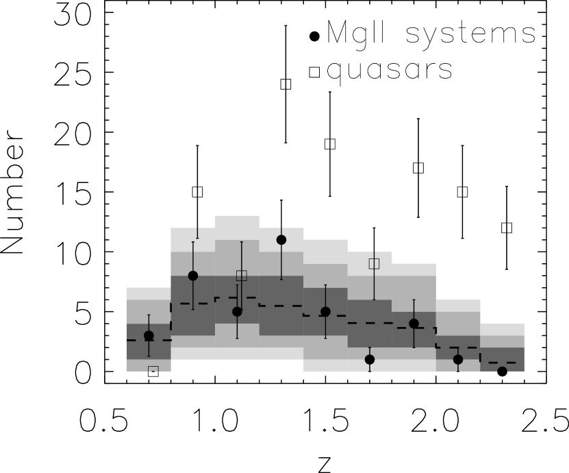
To account for cosmic variance, the number of Mg II absorbers in each random sample was drawn from a Poissonian distribution with a mean equal to the number of absorbers actually observed. For the strong survey, we find no significant deviation from a random distribution (perhaps due to the small sample size). However, for the weak survey, we find an overabundance of Mg II systems at , which is coincident with the Clowes & Campusano large quasar group: we find 11 absorbers, and expect . The Mg II redshift distribution, our selection function and (for reference) the quasar redshift distribution are shown in Fig. 4a. If we assume a Gaussian distribution for the simulated number of absorbers at , this would be a significance of . If we measure the probability directly from the number of simulations, 1.78% of any of the 90000 total redshift bins (9 bins 10000 simulations) produced an overdensity at the level; 2.05% had 11 or more absorbers in the bin. The large quasar group occupies the same redshift interval, which implies that the Mg II and quasar overdensities are related; in fact, despite the various selection methods used for the quasars, the ratio between quasars and Mg II absorbers remains constant (within Poissonian errors of ) over .
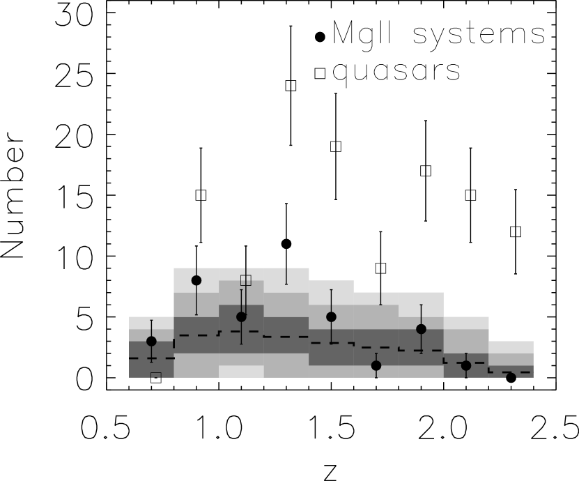
If there is an anomalous concentration of absorbers at a particular redshift, which could be the case if Mg II systems are associated with the large quasar group, then the expected number of Mg II systems in the same redshift range as the large quasar group would be overestimated by the above procedure, and the significance thus underestimated. If we draw 10000 random samples from a Poissonian number distribution with a mean of 24 (which is the expected number from the weak sample given our redshift coverage and the Steidel & Sargent redshift number density), then we would expect Mg II absorbers at , resulting in a overdensity in that redshift bin (Fig. 4b). Only 0.02% of the simulations produced 11 absorbers in that bin, and % produced more; only 0.06% of any of the 90000 bins in any simulation had a significance of 4.3 or higher.
A conservative estimate for the significance of the overdensity at is therefore , though it could be as high as depending on how we normalize our control sample.
4.2 Quasar-Mg II correlations
To test for quasar-Mg II correlations in three dimensions, we calculated the three dimensional two point correlation function between the 107 quasars at in our sample and all of the Mg II absorbers over all redshifts in our survey. We used 10000 control samples with randomized Mg II absorber redshifts similar to those described in the previous section. We found no significant signal for either the strong or weak survey at any scale.
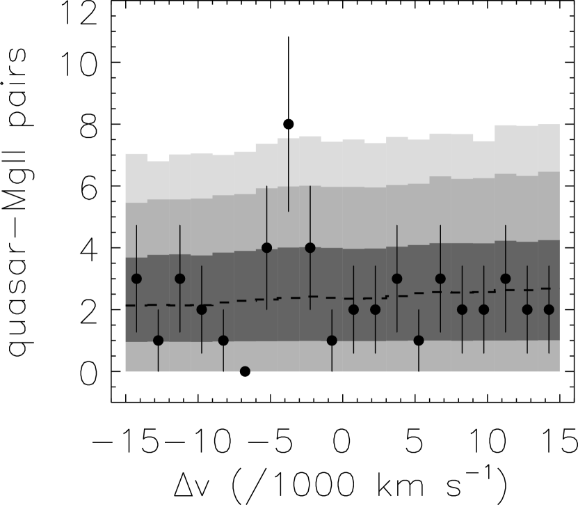
We then tested for correlations in the plane of the sky. Although no such three dimensional large scale correlation has been noted in the literature, there is a precedent for an association between quasars and C IV absorbers at a projected distance of Mpc (Møller 1995; private communication). We cross-correlated the same quasars with the strong and weak Mg II samples, but only along different lines of sight (which avoids effects from associated absorption) for a series of projected separations on the sky covering Mpc in the local frame. Again, we used 10000 control samples with randomized Mg II redshifts, drawing a number from a Poisson distribution with a mean equal to the number of observed absorbers, to determine the mean and standard deviation expected in each bin. As the number of quasar-Mg II pairs varied for each simulated data set, we normalized the total number of pairs for each simulation to that actually observed. There is no significant signal for the strong sample, but for the weak sample we find a signal which peaks at proper (rest frame) Mpc projected separation (35 arcmin at ) at the significance level (8 pairs observed, expected). The overdensity occurs at a velocity difference to km s-1. The negative sign indicates that a quasar is at a lower redshift than its paired Mg II absorber (Fig. 5; Table 5). We expect the peak to be at if the quasar redshifts are accurate, and if quasars and Mg II systems trace mass in a similar way. Only 0.23% of the simulations produced as many as 8 pairs in the to km s-1 velocity bin, with 0.26% of any bins among all of the Monte Carlo simulations producing an equal or greater overdensity of . There is no significant preference for strong or weak systems to be associated with the correlation. Most of the signal (i.e. 5 of 8 pairs) comes from quasars and Mg II absorbers in the large quasar group. Possible physical explanations for the overdensity will be discussed in §5.
It is possible, but unlikely, that the quasar-Mg II absorber pair velocity difference is produced by a systematic quasar offset between quasar rest frame UV and optical lines. Our quasar redshifts were taken either from the Veron-Cetty & Veron (2001) catalogue, measured from our own Å confirmation spectra (Clowes & Campusano, 1994; Clowes, Campusano, & Graham, 1999) or, in the case of 22 of the quasars (all except J104545+0523), from the data presented here. There is no systematic offset between the our two sets of measurements, independent of whether Mg II, C IV, Si IV or C III] emission lines were used. Five of the eight quasar-Mg II pairs at km s-1 have quasar redshifts determined from Mg II emission lines. The other three are from higher ionization C IV or C III] emission lines. McIntosh et al. (1999) and Scott et al. (2000, and references therein) find that quasar Mg II emission provides redshifts within km s-1 of [O III] 5007 (the systemic redshift fiducial), with a correlation between velocity differences and quasar luminosity. However, the observed peak in the distribution of quasar-Mg II absorber pairs is at times larger than would be expected from an offset between Mg II (rest frame UV) and the fiducial [O III] 5007 (rest frame optical) emission. IR spectroscopy of the quasars which produce the quasar-Mg II pair overdensity can confirm or rule out this rather unlikely explanation.
The luminosities of the quasars involved in the correlation are not unusual. The 8 quasars in the overdensity of pairs with to km s-1 have mean absolute magnitude , calculated with code kindly provided by M. Veron-Cetty for the purposes of using a uniform definition of . Our sample of quasars at has , whereas 16892 quasars in the Veron-Cetty & Veron catalogue at the same range have . Our quasar sample is not significantly more luminous than a very large but admittedly inhomogeneous sample, so it is doubtful that a luminosity effect contributes to part of the systematic velocity difference we observe between the quasars and Mg II absorbers. Indeed, the correlation may simply be a fluke due to small number statistics, and should be confirmed with a larger data sample.
4.3 Minimal spanning tree
The minimal spanning tree (MST) is a heuristic algorithm which can delineate and characterize structure within a data set. We have applied the technique of Graham, Clowes, & Campusano (1995) to search for clusters of Mg II absorbers in both the strong and weak samples. An identified cluster is assigned a statistical significance by determining how frequently structures of equivalent multiplicity111Multiplicity is a term used in spatial pattern statistics to denote the number of objects making up a cluster. and with a more clustered morphology occur in 10000 simulations of the data. A simulated absorber position is assigned the right ascension and declination of a randomly selected real absorber to maintain any selection effects in the plane of the sky. Its redshift is determined according to one of three prescriptions: (1) drawn from the observed redshift distribution binned in bins of width ; (2) drawn from the Steidel & Sargent (1992) redshift distribution; and (3) as (2) but with the total number count normalized to the observed number count. For (1), the bins were selected either to match the large quasar group width or to double it, to smooth out Poisson fluctuations on scales of half a bin width or smaller. For (2) and (3), cosmic variance is also taken into account as previously described. No significant structures are found in the strong survey, but a cluster of 10 absorbers is found in the weak survey at redshift . The significance level for the structure from prescription (1) is (0.002) for (0.4); for prescriptions (2) and (3), , 0.01 respectively.
Foreground structure at . At lower redshift, the MST test shows a group of 7 absorbers at with probability to reject that the decision to reject the null hypothesis (that the absorbers are intrinsically unclustered) is wrong of . The exact value of depends on which of the three prescriptions in the preceding paragraph was used to create the control samples. is largely independent of the choice of redshift bin width for the controls (). It appears that at least one of the absorbers is very close (within 1 arcmin) to a galaxy cluster at (Haines, 2001). There is also a structure of 14 quasars at , which is consistent with a random distribution with probability for the observed multiplicity, as determined from a MST analysis of the Chile-UK Quasar Survey (CUQS, Newman, 1999). The probability is again independent of control redshift bin widths. The number of quasars from our sample (Newman, 1999) is lower at , with the probability of any structure arising at of . Thus, the probability of seeing the observed structure at is . The coincidence of the Mg II absorber group, the quasar group and its size, and the proximity of a cluster of red galaxies support the notion of a foreground structure.
5 Discussion
The coincidence of the MgII absorber candidate overabundance with the large quasar group implies that the large quasar group is accompanied by a corresponding increase in galaxy density, possibly similar to those found associated with multiple C IV systems at by Aragón-Salamanca et al. (1994). The MST result provides an independent test which supports the existence of a structure of Mg II absorbers within the large quasar group. The quasar-Mg II correlation may reflect a characteristic size of filaments.
5.1 Mg II absorber overdensity
It may be that Mg II absorbers within the large quasar group could be associated with nearby enhanced ionizing sources such as undetected quasars or AGN. In that case, the halos of the galaxies responsible for the Mg II absorption could possess smaller detectable gas cross sections than in the field, the “galaxy proximity effect” (Pascarelle et al., 2001), which would cause us to underestimate the significance of the Mg II absorber (galaxy) number density in the region. Any mass estimates for the region would also have to take into account that numerical simulations and semi-analytic models show that galaxies should be more highly biased tracers of the mass at higher redshift. If so, then the overdensity of matter in galaxies which produce the Mg II absorption could be closer to the overdensity of matter in super large scale structure of above the mean predicted by Doroshkevich et al. (1999). Estimates of the matter associated with Mg II absorber overdensities could be redshift-dependent: in CDM models, as the amplitude of galaxy clustering remains roughly fixed, the dark matter structure grows with time. Large quasar groups and the galaxies they contain could provide the means to test for such a trend: direct imaging of the Mg II absorbers in the large quasar group should reveal whether there is a tendency for them to occur in areas of higher than average galaxy density, and velocity dispersions of any associated galaxy clusters/groups should constrain the amount of matter in the vicinity. High resolution imaging of Mg II absorbers in the large quasar group could also reveal whether quasars behind the large quasar group are being lensed by galaxies within the large quasar group, which would make it more likely to observe bright background quasars in the region and find foreground Mg II.
Though rare, large structures at have clearly been noted in simulations. Evrard et al. (2001, Hubble volume simulations) find a large cluster at in a CDM model which has a mass twice that of Coma, a line-of-sight velocity dispersion of km s-1 and an equivalent X-ray temperature of 17 keV. It is larger than any known cluster. Although unusual, it might be representative of parts of super large scale structure at . X-ray observations of our large quasar group field, for example around the merging galaxy clusters imaged in the optical and near IR by Haines et al. (2001), would provide the most direct confirmation for such large density perturbations. If baryonic gas evolution can be linked to the dark matter halos in simulations such as that of the Virgo Consortium (which is admittedly difficult, as Mg II arises in galaxies), it could be possible to make mock pencil-beam surveys through the simulated data, and thus make a direct comparison between the observed and predicted size and frequency of large quasar groups and the distribution of galaxies/Mg II absorbers within them. However, it would be more feasible to study Hubble volume simulations of Ly absorbers (which do not necessarily arise in galaxies), and to compare their distribution to the presence of very large structures. In that case, a comparison with observations would require HST spectroscopy for our target field.
A possible non-gravitational origin of such large structures as large quasar groups could be the destruction of H2 or the ionization of He, both of which can be affected over one to several tens Mpc by luminous quasars or other effects of “cooperative galaxy formation” (Miralda-Escudé et al., 2000; Ferrara, 1998; Bower et al., 1993; Kang & Shapiro, 1992; Babul & White, 1992). However, enhanced photoionization has been proposed to impede galaxy formation, at least for low mass halos, by heating the intergalactic medium, inhibiting the collapse of gas into dark halos and reducing the radiative cooling of gas within halos, though galaxies in deep potential wells (brighter than ) appear unaffected (Benson et al., 2001). Large scale perturbations approaching large quasar group size can produce bias on similar size scales, effectively reducing the galaxy formation efficiency in surrounding lower density regions, and thus enhancing the contrast of very large scale structure (Demianski & Doroshkevich, 1999). The effect of inhomogeneous photoionization on structure formation clearly deserves further investigation.
5.2 Quasar–Mg II absorber correlation
The quasar-Mg II absorber correlation may reflect the size of LSS filaments, and is close to the 7 Mpc size of filaments associated with low Ly forest clouds from simulations of structure evolution (Petitjean, Mücket, & Kates, 1995). The angular scale where the peak number of pairs is observed (corresponding to 35 arcmin at ) is consistent with the correlations of up to between AGN and early-type galaxies detected by Brown et al. (2001). We note that five of the eight quasar-Mg II system pairs occur within the large quasar group (). The five large quasar group quasar-Mg II absorber pairs as an ensemble produce most of the significance in the distribution of pairs as a function of velocity (an overdensity at the level), and form a pair and a triplet of quasars of scale 1-10 Mpc, a size on the order of that expected for filamentary structure. The peak at km s-1 should be confirmed with IR spectroscopy of the quasars in question, to rule out the unlikely possibility that the large velocity difference arises from high vs. low ionization line emission regions. Otherwise, the quasars and MgII systems could trace different parts of the same filamentary substructure within the large quasar group. Such a geometry may result as a consequence of the “periphery effect”, in which quasars tend to populate the peripheries of galaxy clusters and metal absorption line groups (Jakobsen & Perryman, 1992; Sánchez & González-Serrano, 1999; Tanaka et al., 2000; Haines et al., 2001; Söchting, Clowes, & Campusano, 2002). In a particularly analogous situation to the large quasar group in this study, Tanaka et al. (2001) detect clustering of faint red galaxies (, ) over a scale extending to 10 Mpc around a tight group of five radio-quiet quasars at , which are embedded in the Crampton, Cowley, & Hartwick (1987, 1989) large quasar group of 23 quasars. Haines et al. (2001) report a similar phenomenon around the quasar J104656+0541 within the large quasar group studied here, albeit in a smaller observed field.
If the periphery effect is the cause of our observed quasar-Mg II correlation at non-zero velocity difference, then we should in principle detect a signal at both positive and negative (according to our definition). However, we only see a negative velocity peak, in which the largest fraction of the signal arises from a set of quasars at separated by arcmin and 4900, 5600 km s-1 in front of a trio of Mg II absorbers separated by 5100, 5700 km s-1 toward two sightlines 29.8 arcmin apart. If the correlation is real, in larger data samples we would expect to find cases of quasars both in front of and behind groups of Mg II absorbers. Alternatively, such a quasar-Mg II correlation which arises for projected distances on the sky, but not in three dimensions, could arise as an effect of peculiar velocities along the line of sight, and may be related to the “bull’s-eye effect” (Praton, Melott, & McKee, 1997; Melott et al., 1998), in which peculiar velocities in collapsing structures tend to make structures more significant in redshift space than in real space. The number of quasar-Mg II pairs in the large quasar group is not sufficient to produce a significant signal on its own, however, and the correlation should be confirmed with a larger sample.
If the quasar-Mg II projected correlation is found to be real, it could be a useful tool to probe the extent and evolution of the overdensities giving rise to quasars themselves. It is possible that quasar clustering declines toward low redshift, as quasar activity moves from the most massive galaxies into lower mass systems that are less highly biased. We expect to continue to find more members of the large quasar group toward ESO/SERC field 927, which will provide better statistics with which to study the relationship between various matter overdensities in the form of quasars, Mg II systems and galaxies.
References
- Aragón-Salamanca et al. (1994) Aragón-Salamanca, A., Ellis, R. S., Schwartzenberg, J.-N., Bergeron, J. A. 1994, ApJ, 421, 27
- Babul & White (1992) Babul, A. & White, S. D. M. 1991, MNRAS, 253, 31P
- Benson et al. (2001) Benson, A. J., Lacey, C. G., Bauth, C. M., Cole, S., & Frenk, C. S. 2001, MNRAS, submitted, astro-ph/0108217
- Best (2000) Best, J. S. 2000, ApJ, 541, 519
- Bower et al. (1993) Bower, R. G., Coles, P., Frenk, C. S., & White, S. D. M. 1993, ApJ, 405, 403
- Brown et al. (2001) Brown, M. J. I., Boyle, B. J., & Webster, R. L. 2001, AJ, 122, 26
- Cen & Simcoe (1997) Cen, R. & Simcoe, R. A. 1997, ApJ, 483, 8
- Davé et al. (1999) Davé, R., Hernquist, L., Katz, N., Weinberg, D. H. 1999, ApJ, 511, 521
- Clowes (2001) Clowes, R. G. 2001, in, “The New Era of Wide Field Astronomy”, Clowes, R. G., Adamson, A., Bromage, G. eds., San Francisco, Astron. Soc. Pacific, ASP Conf Series, Vol. 232.
- Clowes & Campusano (1991) Clowes, R. G. & Campusano, L. E. 1991, MNRAS, 249, 218
- Clowes & Campusano (1994) Clowes, R. G. & Campusano, L. E. 1994, MNRAS, 266, 317
- Clowes, Campusano, & Graham (1995) Clowes, R. G., Campusano L. E., & Graham M. J. 1995, in Maddox S. J., Aragón-Salamanca A., eds, The 35th Herstmonceux Conference, Wide Field Spectroscopy and the Distant Universe. World Scientific Publishing, Singapore, p. 400
- Clowes, Campusano, & Graham (1999) Clowes, R. G., Campusano, L. E., & Graham, M. J. 1999, MNRAS, 309, 48
- Crampton, Cowley, & Hartwick (1987) Crampton D., Cowley A.P., & Hartwick F.D.A. 1987, ApJ, 314, 129
- Crampton, Cowley, & Hartwick (1989) Crampton D., Cowley A.P., & Hartwick F.D.A. 1989, ApJ, 345, 59
- Demianski & Doroshkevich (1999) Demianski, M. & Doroshkevich, A. G. 1999, ApJ, 512, 527
- Demianski & Doroshkevich (2000) Demianski, M. & Doroshkevich, A. G. 2000, MNRAS, 318, 665
- Doroshkevich et al. (2000) Doroshkevich, A. G., Fong, R., McCracken, H. J., Ratcliffe, A., Shanks, T., Turchaninov, V. I. 2000, MNRAS, 315, 767
- Doroshkevich et al. (1999) Doroshkevich, A. G., Müller, V., Retzlaff, J., Turchaninov, V. L. 1999, MNRAS, 306, 575
- Evrard et al. (2001) Evrard, A. E. et al. 2001, ApJ, submitted, astro-ph/0110246
- Ferrara (1998) Ferrara, A. 1998, ApJ, 499, L17
- Francis et al. (2000) Francis, P. J., Williger, G. M., Collins, N. R. et al. 2001, ApJ, 554, 1001
- Fynbo, Møller, & Warren (1999) Fynbo, J. U., Møller, P., & Warren, S. J. 1999, MNRAS, 305, 849
- Geller et al. (1997) Geller, M. J. et al. 1997, AJ, 114, 2205
- Guillemin & Bergeron (1997) Guillemin, P. & Bergeron, J. 1997, A&A, 328, 499
- Graham, Clowes, & Campusano (1995) Graham, M. J., Clowes R. G., & Campusano L. E. 1995, MNRAS 275, 790
- Haines (2001) Haines, C. P. 2001, PhD Thesis, Univ. of Central Lancashire
- Haines et al. (2001) Haines, C. P., Clowes, R. G., Campusano, L. E., Adamson, A. J. 2001, MNRAS, 323, 688
- Jakobsen & Perryman (1992) Jakobsen, P. & Perryman, M. 1992, ApJ, 392, 432
- Kang & Shapiro (1992) Kang, J. & Shapiro, P. R. 1992, ApJ, 386, 432
- Keable (1987) Keable, C. J. 1987, PhD Thesis, Univ. Edinburgh
- Komberg & Lukash (1994) Komberg, B. V. & Lukash, V. N. 1994, MNRAS, 269, 277
- Miralda-Escudé, Haehnelt, & Rees (2000) Miralda-Escudé, J., Haehnelt, M, & Rees, M. J. 2000, ApJ, 530, 1
- McIntosh et al. (1999) McIntosh, D.H., Rix, H.-W., Rieke, M.J., & Foltz, C.B. 1999, ApJ, 517, L73
- Melott et al. (1998) Melott, A. L., Coles, P., Feldman, H. A. & Wilhite, B. 1998, ApJ, 496, L85
- Miralda-Escudé et al. (2000) Miralda-Escudé, J., Haehnelt, M., & Rees, M. J. 2000, ApJ, 530, 1
- Møller (1995) Møller, P. 1995, in “Galaxies in the Young Universe”, eds. Hippelein, H., Meisenheimer, K., Röser, H-J., Springer-Verlag, Heidelberg, Lecture Notes in Physics, V. 463, p. 106
- Møller et al. (2002) Møller, P., Warren, S. J., Fall, S. M., Fynbo, J. U., Jakobsen, P. 2002, ApJ, in press, astro-ph/0203361
- Newman (1999) Newman, P. R. 1999, PhD thesis, Univ. of Central Lancashire
- Newman et al. (1998) Newman, P. R., Clowes, R. G., Campusano, L. E., Graham, M. J. 1998, 14 IAP Astrophys Coll, Éditions Frontieres, p. 408
- Pascarelle et al. (2001) Pascarelle, S. M., Lanzetta, K. M., Chen, H.-W., Webb, J. K. 2001, ApJ, 560, 101
- Petitjean, Mücket, & Kates (1995) Petitjean, P., Mücket, J.P., & Kates, R.E. 1995, A&A, 295, L9
- Pettini et al. (2001) Pettini, M. et al. 2001, ApJ, 554, 981
- Praton, Melott, & McKee (1997) Praton, E. A., Melott, A. L., & McKee, M. Q. 1997, ApJ, 479, 15
- Quashnock et al. (1996) Quashnock, J. M., vanden Berk, D. E., & York, D. G. 1996, ApJ, 472, L69
- Quashnock & Stein (1999) Quashnock, J. M. & Stein, M. L. 1999, ApJ, 515, 506
- Rao & Turnshek (2000) Rao, S. M., & Turnshek, D. A. 2000, ApJS, 130, 1
- Sánchez & González-Serrano (1999) Sánchez, S. & González-Serrano, J. 1999, A&A, 352, 383
- Scott et al. (2000) Scott, J., Bechtold, J., Dobrzycki, A., Kulkarni, V. P. 2000, ApJS, 130, 67
- Silk & Weinberg (1991) Silk, J. & Weinberg, D. 1991, Nature, 350, 272
- Söchting, Clowes, & Campusano (2002) Söchting, I. K., Clowes, R. G., & Campusano, L. E., 2002, MNRAS, 331, 569
- Steidel & Sargent (1992) Steidel, C.C. & Sargent, W.L.W. 1992, ApJS, 80, 1
- Steidel et al. (1997) Steidel, C. C., Dickinson, M., Meyer, D. M., Adelberger, K. L., Sembach, K. R. 1997, ApJ, 480, 568
- Tanaka et al. (2000) Tanaka, I., Yamada, T., Aragón-Salamanca, A., Kodama, T., Miyaji, T., Ohta, K., Arimoto, N. 2000, ApJ, 528, 123
- Tanaka et al. (2001) Tanaka, I., Yamada, T., Turner, E. L., & Suto, Y. 2001, ApJ, 547, 521
- Veron-Cetty & Veron (2001) Véron-Cetty, M.-P., & Veron, P. 2001, A&A, 374, 92
- Warren et al. (2001) Warren, S. J., Møller, P., Fall, S. M., & Jakobsen, P. 2001, MNRAS, 326, 759
- Webster (1982) Webster, A. 1982, MNRAS, 199, 683
- Williger et al. (1996) Williger, G. M., Hazard, C., Baldwin, J.A. & McMahon, R.G., 1996, ApJ Supp, 104, 145
Fig.1: (a-f) Spectra in the quasar sample. The error is shown by the solid line close to the bottom of each plot. The dashed and dotted lines show the wavelengths used for the strong and weak Mg II surveys, respectively. Regions deemed affected by telluric absorption are shaded. Absorption lines are indicated by ticks above the spectrum at (solid) and (dashed) significance; in the telluric bands, only identified extragalactic features are ticked. However, all absorption features are listed in Table 2.
Fig.2: (a-d) Plots of the Mg II doublets in velocity space. Normalized fluxes are shown. The 2803 component is shown offset by -0.2 in flux for clarity. The error array is indicated by the dot-dashed line. The background quasar is listed to the bottom left of each plot, the Mg II absorption redshift is at the bottom center, and four letters indicating the strength of the line (s=strong, w=weak, v=very weak), whether the absorber is in the strong and weak surveys (y/n) and the reality of the system (r=real, c=candidate, d=doubtful), as listed in Table 3. Only “real” systems which are in the strong or weak surveys are used in the analysis for this work.
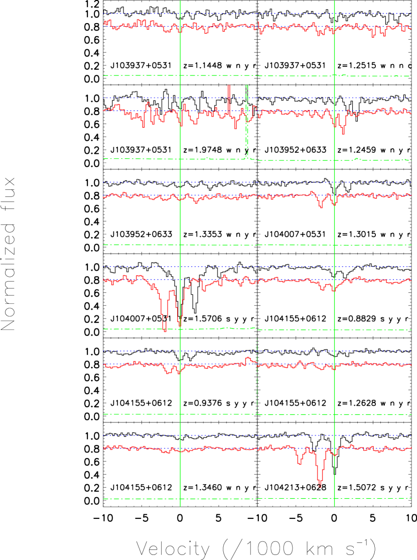
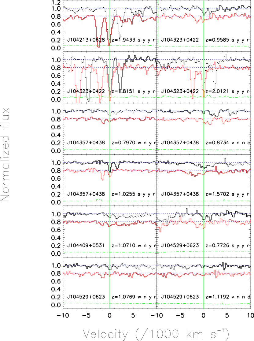
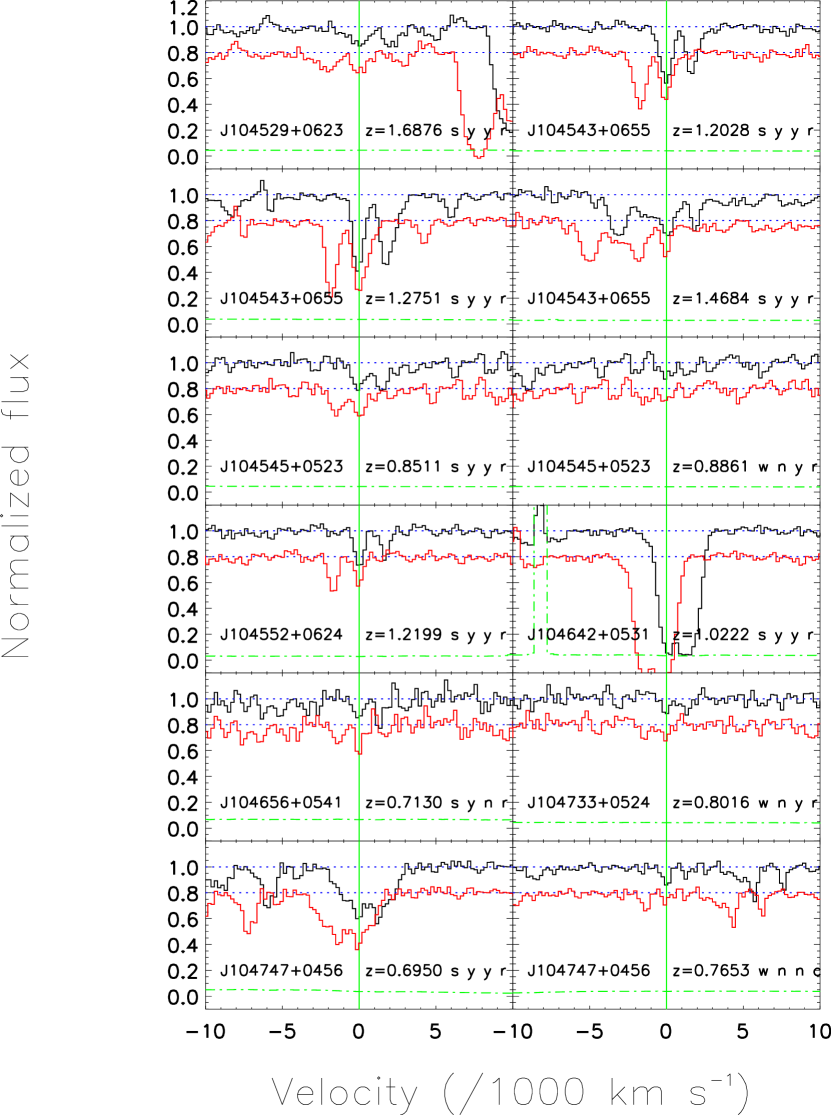
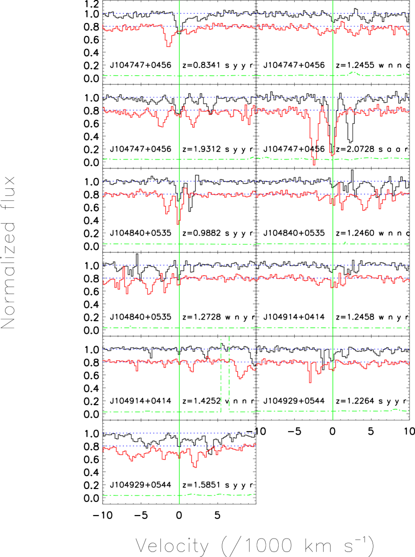
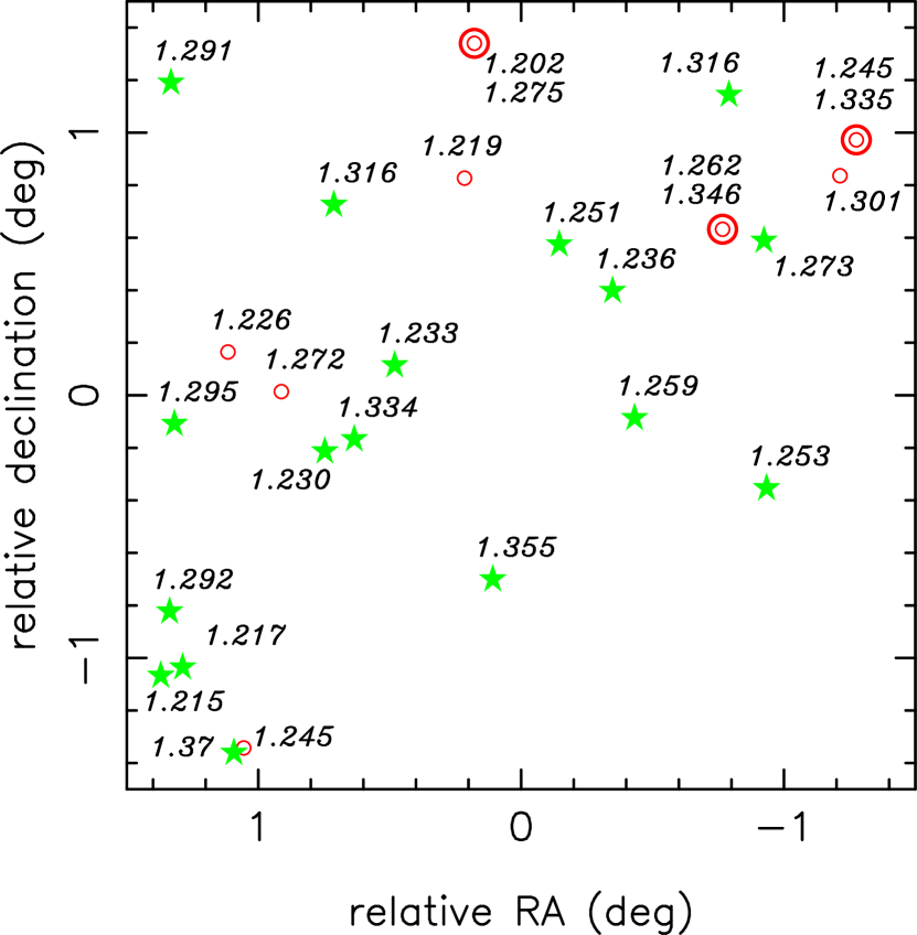
Fig.4:
(a) Redshift distribution of the weak Mg II absorber
sample, compared to simulations of the number observed.
Filled
circles: observed, with errors assuming a Poissonian distribution.
Dashed line: mean expected number per bin from 10000
Monte Carlo simulations, drawn from samples with mean totals equal to the
number observed (38).
Shaded regions: 68, 95, 99% scatter about
the expected mean. The overdensity at , which coincides with
the large quasar group, was matched or exceeded
in 2.05% of the simulations. Open boxes (slightly offset in for clarity): known quasars in
the field, with errors assuming a Poissonian distribution.
(b) Redshift distribution of the weak Mg II absorber
sample, compared to simulations of the number expected.
Filled
circles: observed, with errors assuming a Poissonian distribution.
Dashed line: mean expected number per bin from 10000
Monte Carlo simulations, drawn from samples with mean totals equal to the number
expected (24).
Shaded regions: 68, 95, 99% scatter about
the expected mean. The overdensity at was matched or exceeded
in 0.02% of the simulations. Open boxes (slightly offset in for clarity):
known quasars in the field,
with errors assuming a Poissonian distribution.
| quasar | RA | dec | expb | |||||||
|---|---|---|---|---|---|---|---|---|---|---|
| J2000 | J2000 | (s) | ||||||||
| J103937+0531 | 10:39:37.2 | 05:31:46 | 2.035 | 18.20 | 19.13 | 19.17 | 18.88 | 18.11 | 5d | 9899 |
| J103952+0633 | 10:39:52.2 | 06:33:22 | 1.395 | 18.14 | 18.90 | 18.73 | 18.19 | 18.13 | 4d | 5790 |
| J104007+0531 | 10:40:07.5 | 06:25:09 | 2.383 | 18.05 | 18.54 | 1c | 2400 | |||
| J104117+0610 | 10:41:17.1 | 06:10:17 | 1.273 | 15.42 | 17.03 | 1c | 900 | |||
| J104155+0612 | 10:41:55.7 | 06:12:57 | 1.480 | 18.21 | 19.28 | 3d | 5800 | |||
| J104213+0628 | 10:42:13.5 | 06:28:53 | 2.031 | 18.50 | 19.27 | 19.21 | 19.22 | 18.22 | 3d | 6600 |
| J104213+0619 | 10:42:13.6 | 06:19:42 | 1.560 | 18.73 | 19.24 | 19.09 | 18.60 | 17.87 | 2d | 5700 |
| J104323+0422 | 10:43:23.6 | 04:22:17 | 2.338 | 19.08 | 18.92 | 18.89 | 18.66 | 17.89 | 1c | 3000 |
| J104357+0438 | 10:43:57.8 | 04:38:23 | 2.409 | 18.33 | 18.60 | 18.63 | 18.38 | 17.98 | 3d | 6000 |
| J104409+0531 | 10:44:09.5 | 05:31:34 | 2.110 | 17.95 | 1c | 1500 | ||||
| J104529+0623 | 10:45:29.8 | 06:23:39 | 2.127 | 18.37 | 19.16 | 19.22 | 18.88 | 18.17 | 3d | 9600 |
| J104543+0655 | 10:45:43.6 | 06:55:24 | 2.121 | 18.91 | 19.29 | 19.08 | 18.46 | 17.58 | 7d | 10696 |
| J104545+0523 | 10:45:45.8 | 05:23:55 | 1.751 | 19.11 | 18.37 | 18.08 | 17.96 | 2d | 2500 | |
| J104552+0624 | 10:45:52.7 | 06:24:36 | 1.508 | 17.27 | 17.88 | 18.00 | 17.60 | 17.26 | 1c | 1500 |
| J104642+0531 | 10:46:42.9 | 05:31:06 | 2.681 | 19.58 | 19.18 | 18.85 | 18.23 | 17.52 | 1c | 3600 |
| J104656+0541 | 10:46:56.7 | 05:41:49 | 1.233 | 17.56 | 18.28 | 18.14 | 17.88 | 17.39 | 1c | 1500 |
| J104733+0524 | 10:47:33.2 | 05:24:55 | 1.334 | 16.84 | 17.87 | 1c | 1500 | |||
| J104747+0456 | 10:47:47.1 | 04:56:37 | 2.121 | 18.54 | 19.21 | 19.24 | 18.98 | 18.08 | 1c | 3600 |
| J104752+0618 | 10:47:52.7 | 06:18:28 | 1.316 | 18.28 | 19.12 | 19.16 | 18.56 | 18.18 | 2d | 4800 |
| J104840+0535 | 10:48:40.1 | 05:35:50 | 1.972 | 17.69 | 18.66 | 18.68 | 18.49 | 17.89 | 3d | 5100 |
| J104914+0414 | 10:49:14.3 | 04:14:27 | 1.613 | 18.61 | 19.07 | 19.04 | 18.79 | 18.25 | 2d | 5500 |
| J104929+0544 | 10:49:29.1 | 05:44:53 | 1.802 | 18.77 | 19.07 | 18.97 | 18.57 | 18.02 | 1c | 3000 |
| J105010+0432 | 10:50:10.1 | 04:32:48 | 1.217 | 17.71 | 18.42 | 18.33 | 18.01 | 17.66 | 1c | 2400 |
| Central wavelength | Equivalent | signifb | identification | ||
|---|---|---|---|---|---|
| (Å, vacuum) | width (Å) | /commentsc,d | |||
| J103937+0531 | |||||
| 5569.69 | 0.87 | 1.543 | 0.232 | 6.651 | |
| 5583.63 | 0.51 | 2.014 | 0.221 | 9.113 | |
| 5681.09 | 1.17 | 1.709 | 0.249 | 6.863 | |
| 5997.72 | 1.03 | 0.733 | 0.218 | 3.362 | Mg II 2796 |
| 6012.73 | 0.87 | 0.471 | 0.177 | 2.661 | Mg II 2803 |
| 6295.94 | 0.71 | 1.112 | 0.228 | 4.877 | Mg II 2796 ? (bl) |
| 6314.80 | 1.27 | 0.455 | 0.167 | 2.725 | Mg II 2803 ? (bl) |
| 6358.44 | 0.51 | 0.879 | 0.155 | 5.671 | |
| 6874.77 | 0.26 | 4.527 | 0.189 | 23.952 | |
| 6893.81 | 0.41 | 2.074 | 0.165 | 12.570 | |
| 6907.73 | 0.42 | 1.717 | 0.155 | 11.077 | |
| 6933.59 | 1.08 | 1.261 | 0.197 | 6.401 | |
| 7173.06 | 0.80 | 1.520 | 0.212 | 7.170 | |
| 7187.23 | 0.44 | 1.570 | 0.171 | 9.181 | |
| 7197.53 | 0.40 | 1.372 | 0.158 | 8.684 | |
| 7207.79 | 0.61 | 1.148 | 0.174 | 6.598 | |
| 7234.03 | 1.03 | 1.401 | 0.227 | 6.172 | |
| 7252.61 | 0.56 | 2.257 | 0.219 | 10.306 | |
| 7265.42 | 0.42 | 1.350 | 0.163 | 8.282 | |
| 7281.63 | 0.48 | 1.196 | 0.166 | 7.205 | |
| 7291.23 | 0.77 | 1.023 | 0.196 | 5.219 | |
| 7350.18 | 0.68 | 0.963 | 0.190 | 5.068 | |
| 7607.40 | 0.22 | 17.027 | 0.405 | 42.042 | |
| 7626.89 | 0.16 | 5.146 | 0.233 | 22.086 | |
| 7645.18 | 0.36 | 12.443 | 0.435 | 28.605 | |
| 7923.77 | 0.60 | 3.340 | 0.347 | 9.625 | Mg II 2796 ? |
| (bl; 2803 cpt very weak) | |||||
| 7971.77 | 0.49 | 1.906 | 0.272 | 7.007 | |
| 8000.41 | 0.57 | 2.582 | 0.322 | 8.019 | Mg II 2796 ? |
| (bl; 2803 cpt very weak) | |||||
| 8163.49 | 1.07 | 2.886 | 0.446 | 6.471 | |
| 8232.15 | 0.80 | 1.710 | 0.337 | 5.074 | |
| 8318.53 | 1.34 | 1.297 | 0.335 | 3.872 | Mg II 2796 |
| 8339.77 | 0.64 | 1.114 | 0.248 | 4.492 | Mg II 2803 |
| 8357.90 | 0.92 | 2.007 | 0.356 | 5.638 | |
| 8407.43 | 0.65 | 1.850 | 0.296 | 6.250 | |
| 8423.14 | 0.60 | 1.415 | 0.247 | 5.729 | |
| 8440.43 | 0.79 | 1.878 | 0.288 | 6.521 | |
| 8471.81 | 0.74 | 1.373 | 0.253 | 5.427 | |
| 8767.05 | 0.75 | 3.976 | 0.516 | 7.705 | |
| J103952+0633 | |||||
| 5840.62 | 0.60 | 0.553 | 0.143 | 3.867 | Fe II 2600 |
| 5873.53 | 1.30 | 1.185 | 0.223 | 5.314 | |
| 6280.34 | 0.81 | 0.739 | 0.173 | 4.272 | Mg II 2796 |
| 6296.15 | 0.48 | 1.522 | 0.181 | 8.409 | Mg II 2803 (bl) |
| 6306.73 | 0.37 | 2.333 | 0.252 | 9.258 | |
| 6529.33 | 1.30 | 0.792 | 0.198 | 4.000 | Mg II 2796 |
| 6547.39 | 0.97 | 0.726 | 0.174 | 4.172 | Mg II 2803 |
| 6567.63 | 1.08 | 1.209 | 0.205 | 5.898 | |
| 6873.75 | 0.45 | 2.475 | 0.214 | 11.565 | |
| 7253.49 | 1.12 | 1.773 | 0.288 | 6.156 | |
| 7607.59 | 0.22 | 15.994 | 0.390 | 41.010 | |
| 7631.31 | 0.21 | 8.257 | 0.299 | 27.615 | |
| 7650.74 | 0.42 | 8.467 | 0.389 | 21.766 | |
| 8374.97 | 0.61 | 1.626 | 0.285 | 5.705 | |
| J104007+0531 | |||||
| 4662.20 | 0.60 | 0.975 | 0.254 | 3.839 | Mg I 2026 ? |
| 4672.59 | 0.65 | 1.997 | 0.324 | 6.164 | |
| 4683.31 | 0.85 | 1.885 | 0.348 | 5.417 | |
| 4894.71 | 0.60 | 1.912 | 0.332 | 5.759 | |
| 4910.54 | 0.36 | 7.504 | 0.428 | 17.533 | |
| 4926.65 | 0.27 | 6.961 | 0.366 | 19.019 | |
| 4942.36 | 0.65 | 5.242 | 0.452 | 11.597 | |
| 5005.92 | 0.85 | 10.295 | 0.608 | 16.933 | |
| 5042.72 | 1.01 | 2.400 | 0.383 | 6.266 | |
| 5076.51 | 0.51 | 1.792 | 0.267 | 6.712 | |
| 5091.45 | 1.03 | 4.521 | 0.447 | 10.114 | |
| 5199.92 | 0.47 | 5.376 | 0.275 | 19.549 | |
| 5985.62 | 1.64 | 0.679 | 0.242 | 2.806 | Fe II 2600 ? |
| 6025.13 | 0.52 | 2.492 | 0.249 | 10.008 | Fe II 2344 |
| 6125.02 | 0.29 | 3.566 | 0.227 | 15.709 | Fe II 2383 |
| 6279.74 | 0.80 | 1.002 | 0.199 | 5.035 | |
| 6436.51 | 0.49 | 1.302 | 0.157 | 8.293 | Mg II 2796 |
| 6452.25 | 0.38 | 0.980 | 0.128 | 7.656 | Mg II 2803 |
| 6648.69 | 0.38 | 2.137 | 0.199 | 10.739 | Fe II 2587 |
| 6669.82 | 0.49 | 1.992 | 0.213 | 9.352 | |
| 6683.70 | 0.34 | 3.355 | 0.220 | 15.250 | Fe II 2600 |
| 6874.18 | 0.34 | 3.403 | 0.222 | 15.329 | |
| 6894.76 | 0.84 | 2.118 | 0.258 | 8.209 | |
| 7185.86 | 0.33 | 8.898 | 0.296 | 30.061 | Mg II 2796 (bl) |
| 7206.79 | 0.27 | 7.317 | 0.260 | 28.142 | Mg II 2803 |
| 7239.46 | 1.14 | 1.541 | 0.305 | 5.052 | |
| 7607.35 | 0.16 | 16.446 | 0.271 | 60.686 | |
| 7642.49 | 0.29 | 18.384 | 0.358 | 51.352 | |
| 7682.27 | 0.78 | 2.952 | 0.286 | 10.322 | |
| 8231.52 | 0.71 | 2.153 | 0.266 | 8.094 | |
| 8990.29 | 0.74 | 2.965 | 0.381 | 7.782 | |
| 9006.93 | 0.80 | 2.159 | 0.376 | 5.742 | |
| 9086.04 | 0.89 | 1.573 | 0.304 | 5.174 | |
| 9178.15 | 0.44 | 1.199 | 0.232 | 5.168 | |
| J104117+0610 | |||||
| 4941.03 | 0.28 | 0.791 | 0.126 | 6.278 | |
| 6874.27 | 0.29 | 5.115 | 0.186 | 27.500 | |
| 6892.20 | 0.26 | 2.392 | 0.133 | 17.985 | |
| 6907.82 | 0.36 | 2.859 | 0.162 | 17.648 | |
| 6923.93 | 0.39 | 1.062 | 0.120 | 8.850 | |
| 6934.03 | 0.43 | 0.933 | 0.116 | 8.043 | |
| 6942.85 | 0.36 | 0.835 | 0.105 | 7.952 | |
| 6954.61 | 0.61 | 1.515 | 0.160 | 9.469 | |
| 6997.40 | 0.69 | 1.521 | 0.165 | 9.218 | |
| 7022.00 | 0.68 | 0.936 | 0.138 | 6.783 | |
| 7174.44 | 0.54 | 1.485 | 0.155 | 9.581 | |
| 7189.29 | 0.35 | 1.811 | 0.138 | 13.123 | |
| 7204.02 | 0.51 | 1.834 | 0.163 | 11.252 | |
| 7237.41 | 0.67 | 0.705 | 0.137 | 5.146 | |
| 7278.62 | 0.68 | 1.151 | 0.169 | 6.811 | |
| 7292.02 | 0.72 | 0.820 | 0.146 | 5.616 | |
| 7308.47 | 0.83 | 0.874 | 0.157 | 5.567 | |
| 7566.52 | 0.91 | 0.803 | 0.159 | 5.050 | |
| 7607.47 | 0.10 | 16.496 | 0.188 | 87.745 | |
| 7640.97 | 0.22 | 16.928 | 0.260 | 65.108 | |
| 7673.15 | 0.40 | 1.109 | 0.129 | 8.597 | |
| 7683.59 | 0.57 | 0.810 | 0.133 | 6.090 | |
| 8152.73 | 0.88 | 1.473 | 0.224 | 6.576 | |
| 8167.96 | 0.74 | 1.225 | 0.196 | 6.250 | |
| 8182.55 | 0.66 | 1.162 | 0.190 | 6.116 | |
| 8233.64 | 0.43 | 2.685 | 0.222 | 12.095 | |
| 8295.65 | 0.48 | 1.358 | 0.226 | 6.009 | |
| 8324.75 | 1.17 | 1.392 | 0.257 | 5.416 | |
| 8992.45 | 0.37 | 1.456 | 0.235 | 6.196 | |
| 9157.19 | 0.86 | 2.007 | 0.333 | 6.027 | |
| J104155+0612 | |||||
| 4617.26 | 0.92 | 0.864 | 0.196 | 4.408 | Fe II 2383 (bl) |
| 5262.48 | 0.69 | 1.756 | 0.174 | 10.092 | Mg II 2796 (bl) |
| 5279.90 | 0.54 | 1.946 | 0.165 | 11.794 | Mg II 2803 |
| 5417.93 | 0.46 | 1.384 | 0.138 | 10.029 | Mg II 2796 |
| 5432.21 | 0.71 | 1.222 | 0.151 | 8.093 | Mg II 2803 |
| 5531.16 | 0.66 | 0.804 | 0.131 | 6.137 | Mg I 2852 (bl) |
| 5561.91 | 0.89 | 0.671 | 0.130 | 5.162 | |
| 5887.21 | 0.85 | 0.958 | 0.141 | 6.794 | |
| 5906.31 | 0.69 | 0.540 | 0.107 | 5.047 | |
| 6327.06 | 0.62 | 0.849 | 0.115 | 7.383 | Mg II 2796 |
| 6342.97 | 0.88 | 0.725 | 0.123 | 5.894 | Mg II 2803 |
| 6559.49 | 0.88 | 0.742 | 0.126 | 5.889 | Mg II 2796 |
| 6576.77 | 0.98 | 0.559 | 0.118 | 4.737 | Mg II 2803 |
| 6875.11 | 0.24 | 3.649 | 0.138 | 26.442 | |
| 6896.83 | 0.98 | 1.504 | 0.159 | 9.459 | |
| 7607.47 | 0.20 | 15.239 | 0.292 | 52.188 | |
| 7642.19 | 0.35 | 17.754 | 0.374 | 47.471 | |
| 7800.37 | 0.76 | 0.972 | 0.184 | 5.283 | |
| 8164.86 | 0.95 | 1.709 | 0.257 | 6.650 | |
| 8200.24 | 1.16 | 1.478 | 0.271 | 5.454 | |
| 8230.23 | 0.63 | 2.309 | 0.253 | 9.126 | |
| 8770.24 | 0.49 | 1.960 | 0.279 | 7.025 | |
| 8891.98 | 1.12 | 2.581 | 0.417 | 6.189 | |
| 8991.11 | 0.72 | 3.068 | 0.385 | 7.969 | |
| 9014.77 | 1.56 | 2.473 | 0.477 | 5.184 | |
| J104213+0628 | |||||
| 4636.78 | 0.35 | 3.847 | 0.259 | 14.853 | |
| 4648.04 | 0.45 | 3.781 | 0.245 | 15.433 | |
| 4669.49 | 0.74 | 0.833 | 0.153 | 5.444 | |
| 4729.72 | 0.86 | 2.936 | 0.292 | 10.055 | Fe II 1608 (bl) |
| 4917.36 | 0.52 | 2.589 | 0.232 | 11.159 | Al II 1670 |
| 5086.27 | 0.79 | 0.971 | 0.165 | 5.885 | |
| 5134.07 | 0.33 | 0.823 | 0.119 | 6.916 | |
| 5320.27 | 1.15 | 0.644 | 0.160 | 4.025 | Si II 1808 ? |
| S I 1803 ? | |||||
| 5455.91 | 0.87 | 0.630 | 0.159 | 3.962 | Al III 1855 ? |
| 5536.95 | 0.31 | 1.020 | 0.137 | 7.445 | |
| 5581.36 | 0.39 | 1.037 | 0.174 | 5.960 | |
| 6564.21 | 0.24 | 0.641 | 0.089 | 7.202 | |
| 6873.74 | 0.38 | 3.087 | 0.185 | 16.686 | |
| 6897.79 | 0.32 | 5.329 | 0.211 | 25.256 | Fe II 2344 |
| 6987.87 | 0.33 | 1.868 | 0.152 | 12.289 | Fe II 2374 |
| 7011.50 | 0.25 | 5.304 | 0.194 | 27.340 | Mg II 2796 , |
| Fe II 2383 (bl) | |||||
| 7028.62 | 0.70 | 0.836 | 0.146 | 5.726 | Mg II 2803 |
| 7195.83 | 0.66 | 0.763 | 0.146 | 5.226 | |
| 7606.77 | 0.18 | 16.070 | 0.291 | 55.223 | |
| 7629.57 | 0.19 | 7.815 | 0.233 | 33.541 | |
| 7653.95 | 0.37 | 11.034 | 0.334 | 33.036 | Fe II 2600 |
| 8230.49 | 0.23 | 8.122 | 0.319 | 25.461 | Mg II 2796 |
| 8251.27 | 0.33 | 7.438 | 0.351 | 21.191 | Mg II 2803 |
| 8280.89 | 0.89 | 2.044 | 0.315 | 6.489 | |
| 8323.14 | 1.23 | 1.900 | 0.338 | 5.621 | |
| 8355.79 | 0.66 | 1.578 | 0.258 | 6.116 | |
| 8394.65 | 0.70 | 1.347 | 0.234 | 5.756 | Mg I 2852 |
| 8630.36 | 1.47 | 1.988 | 0.390 | 5.097 | |
| 8667.91 | 0.92 | 2.198 | 0.352 | 6.244 | |
| 9108.49 | 0.62 | 1.721 | 0.309 | 5.570 | |
| J104213+0619 | |||||
| 4668.71 | 0.70 | 1.524 | 0.265 | 5.751 | |
| 4787.50 | 0.78 | 0.747 | 0.144 | 5.188 | |
| 4798.76 | 0.73 | 0.742 | 0.135 | 5.496 | |
| 4818.97 | 0.81 | 1.745 | 0.244 | 7.152 | |
| 4866.27 | 0.83 | 1.189 | 0.131 | 9.076 | |
| 4916.56 | 1.15 | 0.906 | 0.140 | 6.471 | |
| 6282.88 | 0.97 | 1.143 | 0.148 | 7.723 | |
| 6874.80 | 0.26 | 3.085 | 0.152 | 20.296 | |
| 6893.95 | 0.54 | 1.939 | 0.166 | 11.681 | |
| 6907.41 | 0.50 | 0.815 | 0.118 | 6.907 | |
| 6918.80 | 0.75 | 0.696 | 0.129 | 5.395 | |
| 7198.82 | 0.90 | 2.474 | 0.194 | 12.753 | |
| 7236.26 | 0.79 | 0.747 | 0.146 | 5.116 | |
| 7607.89 | 0.20 | 15.031 | 0.279 | 53.875 | |
| 7642.38 | 0.35 | 15.899 | 0.348 | 45.687 | |
| 7723.50 | 1.08 | 1.199 | 0.225 | 5.329 | |
| 8233.02 | 0.83 | 2.116 | 0.307 | 6.893 | |
| 8890.62 | 0.98 | 2.328 | 0.398 | 5.849 | |
| 8967.70 | 0.65 | 1.587 | 0.299 | 5.308 | |
| 9058.41 | 0.79 | 1.684 | 0.330 | 5.103 | |
| 9105.85 | 0.99 | 2.711 | 0.422 | 6.424 | |
| J104323+0422 | |||||
| 4667.44 | 0.56 | 3.837 | 0.311 | 12.338 | Fe II 2383 ?, |
| CI 1657 ?, | |||||
| CIV 1548/1550 ? (bl) | |||||
| 4705.27 | 0.38 | 4.293 | 0.286 | 15.010 | Al II 1671 |
| 5033.88 | 0.49 | 2.271 | 0.239 | 9.502 | Al II 1671 ? (bl) |
| 5092.36 | 1.17 | 0.565 | 0.191 | 2.958 | Fe II 2600 |
| 5222.99 | 0.55 | 1.954 | 0.209 | 9.349 | Al III 1855 |
| 5243.75 | 1.22 | 1.134 | 0.240 | 4.725 | Al III 1863 ; |
| Ni II 1742 ? (bl) | |||||
| 5477.48 | 0.76 | 1.454 | 0.214 | 6.794 | Mg II 2796 |
| 5490.31 | 0.59 | 0.963 | 0.164 | 5.872 | Mg II 2803 |
| 5606.34 | 0.70 | 1.384 | 0.209 | 6.622 | |
| 6363.71 | 0.82 | 0.699 | 0.165 | 4.236 | Fe II 2261 |
| 6419.84 | 1.30 | 1.084 | 0.204 | 5.314 | |
| 6600.02 | 0.27 | 3.835 | 0.198 | 19.369 | Fe II 2344 |
| 6685.02 | 0.44 | 3.038 | 0.211 | 14.398 | Fe II 2374 |
| 6708.32 | 0.19 | 4.978 | 0.187 | 26.620 | Fe II 2383 |
| 6875.17 | 0.38 | 2.767 | 0.205 | 13.498 | |
| 6893.81 | 1.15 | 1.078 | 0.214 | 5.037 | |
| 7060.68 | 0.19 | 2.229 | 0.146 | 15.267 | Fe II 2344 |
| 7153.05 | 0.79 | 1.143 | 0.196 | 5.832 | Fe II 2374 (bl) |
| 7176.85 | 0.23 | 4.925 | 0.198 | 24.874 | Fe II 2383 (bl) |
| 7188.89 | 0.31 | 1.629 | 0.146 | 11.158 | |
| 7202.35 | 0.46 | 2.488 | 0.197 | 12.629 | |
| 7236.88 | 0.68 | 1.830 | 0.239 | 7.657 | |
| 7255.71 | 0.48 | 1.588 | 0.190 | 8.358 | Mn II 2577 |
| 7266.80 | 0.60 | 0.910 | 0.158 | 5.759 | |
| 7282.02 | 0.35 | 5.376 | 0.297 | 18.101 | Fe II 2587 |
| 7305.65 | 0.57 | 1.359 | 0.191 | 7.115 | Mn II 2594 |
| 7320.58 | 0.26 | 5.736 | 0.259 | 22.147 | Fe II 2600 |
| 7336.50 | 0.88 | 1.293 | 0.246 | 5.256 | Mn II 2606 (bl) |
| 7349.42 | 0.74 | 1.127 | 0.208 | 5.418 | |
| 7607.03 | 0.16 | 15.576 | 0.257 | 60.607 | |
| 7632.53 | 0.16 | 9.512 | 0.223 | 42.655 | |
| 7653.80 | 0.40 | 6.556 | 0.281 | 23.331 | |
| 7790.19 | 0.43 | 2.251 | 0.239 | 9.418 | Fe II 2587 (bl) |
| 7829.39 | 0.10 | 9.348 | 0.208 | 44.942 | Fe II 2600 |
| 7872.12 | 0.33 | 7.783 | 0.370 | 21.035 | Mg II 2796 |
| 7893.07 | 0.20 | 7.206 | 0.274 | 26.299 | Mg II 2803 |
| 8033.92 | 0.85 | 1.509 | 0.277 | 5.448 | Mg I 2852 |
| 8164.45 | 1.38 | 1.571 | 0.290 | 5.417 | |
| 8232.17 | 0.45 | 2.279 | 0.224 | 10.174 | |
| 8279.64 | 1.15 | 2.152 | 0.392 | 5.490 | |
| 8341.03 | 0.75 | 2.150 | 0.347 | 6.196 | |
| 8352.79 | 0.85 | 2.145 | 0.397 | 5.403 | |
| 8422.64 | 0.34 | 5.803 | 0.339 | 17.118 | Mg II 2796 |
| 8445.00 | 0.38 | 5.825 | 0.320 | 18.203 | Mg II 2803 |
| 8593.56 | 0.71 | 1.376 | 0.242 | 5.686 | Mg I 2852 |
| 9135.55 | 0.58 | 1.546 | 0.259 | 5.969 | |
| 9155.95 | 1.08 | 2.223 | 0.378 | 5.881 | |
| J104357+0438 | |||||
| 5024.69 | 0.80 | 0.797 | 0.158 | 5.044 | Mg II 2796 |
| 5038.07 | 1.15 | 0.676 | 0.168 | 4.024 | Mg II 2803 |
| 5238.75 | 0.71 | 0.275 | 0.085 | 3.235 | Mg II 2796 |
| 5255.08 | 0.34 | 0.891 | 0.089 | 10.011 | Mg II 2803 (bl) |
| 5264.85 | 0.23 | 1.222 | 0.081 | 15.086 | Mg II 2796 ? |
| + Fe II2600 (bl) | |||||
| 5292.51 | 0.34 | 0.626 | 0.074 | 8.459 | |
| 5301.70 | 0.65 | 0.469 | 0.088 | 5.330 | |
| 5664.06 | 0.41 | 1.385 | 0.125 | 11.080 | Mg II 2796 |
| 5678.71 | 0.46 | 1.059 | 0.120 | 8.825 | Mg II 2803 |
| 5777.71 | 1.08 | 0.915 | 0.157 | 5.828 | Mg I 2852 |
| 5894.71 | 0.93 | 0.888 | 0.143 | 6.210 | |
| 6297.34 | 0.76 | 0.731 | 0.138 | 5.297 | |
| 6874.70 | 0.27 | 3.923 | 0.168 | 23.351 | |
| 6894.46 | 0.40 | 2.587 | 0.162 | 15.969 | |
| 6909.81 | 0.44 | 0.898 | 0.114 | 7.877 | |
| 6932.87 | 0.95 | 1.544 | 0.181 | 8.530 | |
| 6955.02 | 0.91 | 0.804 | 0.141 | 5.702 | |
| 7172.04 | 0.87 | 0.933 | 0.141 | 6.617 | |
| 7187.80 | 0.42 | 1.946 | 0.143 | 13.608 | Mg II 2796 (bl) |
| 7203.78 | 0.66 | 1.284 | 0.146 | 8.795 | Mg II 2803 |
| 7248.06 | 0.94 | 0.960 | 0.157 | 6.115 | |
| 7607.10 | 0.14 | 15.501 | 0.248 | 62.504 | |
| 7634.09 | 0.17 | 11.365 | 0.238 | 47.752 | |
| 7659.26 | 0.40 | 6.611 | 0.267 | 24.760 | |
| 7697.25 | 0.81 | 1.469 | 0.208 | 7.062 | |
| 7830.18 | 0.39 | 0.333 | 0.113 | 2.947 | Mg II 2796 ? |
| 8166.43 | 0.78 | 0.942 | 0.181 | 5.204 | |
| 8201.58 | 0.67 | 1.065 | 0.177 | 6.017 | |
| 8230.63 | 0.77 | 1.384 | 0.206 | 6.718 | |
| 8834.54 | 0.20 | 0.718 | 0.127 | 5.654 | |
| J104409+0531 | |||||
| 4668.79 | 0.78 | 2.040 | 0.277 | 7.365 | |
| 4815.80 | 0.21 | 1.039 | 0.128 | 8.117 | |
| 4981.05 | 0.38 | 1.271 | 0.167 | 7.611 | |
| 5808.31 | 0.78 | 1.470 | 0.182 | 8.077 | |
| 5826.56 | 0.64 | 1.297 | 0.160 | 8.106 | |
| 5842.15 | 0.71 | 1.156 | 0.159 | 7.270 | |
| 5791.13 | 0.95 | 0.750 | 0.155 | 4.839 | Mg II 2796 |
| 5808.31 | 0.78 | 1.470 | 0.182 | 8.077 | Mg II 2803 |
| 6277.99 | 0.70 | 1.599 | 0.194 | 8.242 | |
| 6597.23 | 0.91 | 0.886 | 0.176 | 5.034 | |
| 6875.04 | 0.41 | 3.324 | 0.217 | 15.318 | |
| 6889.63 | 0.57 | 0.674 | 0.134 | 5.030 | |
| 6902.20 | 0.86 | 1.592 | 0.216 | 7.370 | |
| 6963.35 | 0.71 | 0.961 | 0.169 | 5.686 | |
| 7027.06 | 0.63 | 0.868 | 0.158 | 5.494 | |
| 7176.63 | 0.62 | 0.833 | 0.149 | 5.591 | |
| 7188.17 | 0.46 | 1.667 | 0.165 | 10.103 | |
| 7198.49 | 0.37 | 0.983 | 0.124 | 7.927 | |
| 7206.17 | 0.62 | 0.832 | 0.149 | 5.584 | |
| 7413.59 | 0.77 | 0.926 | 0.178 | 5.202 | |
| 7563.14 | 0.76 | 0.934 | 0.175 | 5.337 | |
| 7607.26 | 0.17 | 16.141 | 0.243 | 66.424 | |
| 7641.85 | 0.29 | 17.679 | 0.319 | 55.420 | |
| 7679.28 | 0.47 | 0.816 | 0.133 | 6.135 | |
| 7695.45 | 0.73 | 1.172 | 0.185 | 6.335 | |
| 8230.71 | 0.31 | 2.199 | 0.198 | 11.106 | |
| 8991.03 | 0.66 | 1.785 | 0.294 | 6.071 | |
| 9073.02 | 0.52 | 1.287 | 0.235 | 5.477 | |
| 9134.65 | 0.51 | 1.317 | 0.235 | 5.604 | |
| 9178.82 | 0.54 | 1.607 | 0.249 | 6.454 | |
| J104529+0623 | |||||
| 4764.66 | 1.21 | 1.525 | 0.291 | 5.241 | |
| 4819.66 | 0.24 | 6.105 | 0.180 | 33.917 | |
| 4842.84 | 0.24 | 1.353 | 0.095 | 14.242 | |
| 4851.02 | 0.37 | 0.872 | 0.094 | 9.277 | |
| 4875.50 | 0.51 | 4.063 | 0.212 | 19.165 | |
| 4895.32 | 0.80 | 0.951 | 0.189 | 5.032 | |
| 4956.87 | 0.96 | 1.310 | 0.274 | 4.781 | Mg II 2796 |
| 4968.93 | 0.94 | 1.107 | 0.257 | 4.307 | Mg II 2803 |
| 5144.16 | 0.64 | 0.959 | 0.178 | 5.388 | |
| 5153.51 | 0.56 | 1.075 | 0.173 | 6.214 | |
| 5555.66 | 0.60 | 1.107 | 0.192 | 5.766 | |
| 5576.94 | 0.49 | 2.631 | 0.278 | 9.464 | |
| 5585.46 | 0.42 | 0.818 | 0.148 | 5.527 | |
| 5807.68 | 0.70 | 1.019 | 0.177 | 5.757 | Mg II 2796 (bl) |
| 5822.67 | 1.20 | 0.583 | 0.173 | 3.370 | Mg II 2803 |
| 5897.69 | 1.17 | 1.206 | 0.188 | 6.415 | |
| 5926.09 | 1.01 | 0.573 | 0.126 | 4.548 | Mg II 2796 |
| 5943.24 | 1.06 | 0.793 | 0.133 | 5.962 | Mg II 2803 |
| 5967.20 | 0.13 | 0.414 | 0.046 | 9.000 | |
| 5993.73 | 1.41 | 0.801 | 0.151 | 5.305 | |
| 6874.56 | 0.31 | 4.350 | 0.233 | 18.670 | |
| 6889.71 | 0.35 | 2.161 | 0.186 | 11.618 | |
| 6902.10 | 0.56 | 1.995 | 0.215 | 9.279 | |
| 6918.61 | 0.75 | 1.053 | 0.195 | 5.400 | |
| 6950.85 | 0.77 | 1.021 | 0.196 | 5.209 | |
| 7514.30 | 1.23 | 2.145 | 0.326 | 6.580 | Mg II 2796 |
| 7535.84 | 0.92 | 1.717 | 0.274 | 6.266 | Mg II 2803 |
| 7608.03 | 0.18 | 16.702 | 0.342 | 48.836 | |
| 7627.16 | 0.14 | 4.892 | 0.201 | 24.338 | |
| 7648.34 | 0.40 | 14.046 | 0.424 | 33.127 | |
| 7758.35 | 0.61 | 1.592 | 0.241 | 6.606 | |
| 7885.48 | 1.40 | 2.068 | 0.360 | 5.744 | |
| 7927.10 | 0.70 | 1.426 | 0.249 | 5.727 | |
| 8165.16 | 1.01 | 1.826 | 0.357 | 5.115 | |
| 8231.78 | 0.82 | 1.923 | 0.341 | 5.639 | |
| 8281.22 | 0.82 | 3.113 | 0.404 | 7.705 | |
| 8346.12 | 0.56 | 3.598 | 0.388 | 9.273 | |
| 8459.58 | 0.68 | 1.695 | 0.334 | 5.075 | |
| 8766.22 | 0.67 | 4.400 | 0.339 | 12.979 | |
| 8839.01 | 0.45 | 4.599 | 0.398 | 11.555 | |
| 8890.24 | 0.74 | 4.739 | 0.505 | 9.384 | |
| 8925.27 | 0.89 | 3.650 | 0.515 | 7.087 | |
| 8956.31 | 0.75 | 2.353 | 0.436 | 5.397 | |
| 8966.35 | 0.77 | 2.396 | 0.460 | 5.209 | |
| J104543+0655 | |||||
| 5082.38 | 1.13 | 1.507 | 0.247 | 6.101 | |
| 5163.85 | 0.73 | 1.610 | 0.225 | 7.156 | Fe II 2344 (bl) |
| 5249.28 | 0.72 | 2.055 | 0.258 | 7.965 | Fe II 2383 |
| 5333.13 | 0.33 | 3.327 | 0.240 | 13.863 | Fe II 2344 |
| 5401.96 | 0.35 | 2.844 | 0.219 | 12.986 | Fe II 2374 |
| 5421.10 | 0.53 | 4.886 | 0.298 | 16.396 | Fe II 2383 |
| 5583.38 | 0.56 | 1.184 | 0.231 | 5.126 | |
| 5697.37 | 1.01 | 0.713 | 0.208 | 3.428 | Fe II 2587 |
| 5727.68 | 0.50 | 2.171 | 0.235 | 9.238 | Fe II 2600 |
| 5785.31 | 0.66 | 1.018 | 0.194 | 5.247 | Fe II 2344 |
| 5860.84 | 0.64 | 1.160 | 0.183 | 6.339 | Fe II 2374 ; |
| Mn II 2577 ? (bl) | |||||
| 5883.41 | 0.26 | 5.521 | 0.228 | 24.215 | Fe II 2587 , |
| Fe II2383 (bl) | |||||
| 5902.81 | 0.68 | 0.587 | 0.138 | 4.254 | Mn II 2594 ? (bl |
| 5917.79 | 0.49 | 5.669 | 0.252 | 22.496 | Fe II 2600 |
| 6159.68 | 0.31 | 3.822 | 0.231 | 16.545 | Mg II 2796 |
| 6175.99 | 0.43 | 3.189 | 0.236 | 13.513 | Mg II 2803 |
| 6282.55 | 1.41 | 2.343 | 0.318 | 7.368 | Mg I 2852 |
| 6361.95 | 0.32 | 5.149 | 0.240 | 21.454 | Mg II 2796 |
| 6380.18 | 0.30 | 6.016 | 0.240 | 25.067 | Mg II 2803 , |
| Fe II2587 (bl) | |||||
| 6417.60 | 0.53 | 1.334 | 0.176 | 7.580 | Fe II 2600 |
| 6490.56 | 0.50 | 1.943 | 0.188 | 10.335 | Mg I 2852 |
| 6874.05 | 0.28 | 3.996 | 0.180 | 22.200 | |
| 6888.16 | 0.28 | 1.174 | 0.114 | 10.298 | |
| 6902.13 | 0.30 | 4.360 | 0.189 | 23.069 | Mg II 2796 |
| 6920.69 | 0.40 | 2.065 | 0.161 | 12.826 | Mg II 2803 |
| 6936.36 | 0.75 | 0.747 | 0.140 | 5.336 | |
| 6955.57 | 0.75 | 0.798 | 0.148 | 5.392 | |
| 7046.56 | 0.69 | 0.655 | 0.130 | 5.038 | |
| 7187.76 | 0.72 | 0.835 | 0.148 | 5.642 | |
| 7202.23 | 1.04 | 1.558 | 0.216 | 7.213 | |
| 7280.76 | 0.86 | 0.943 | 0.175 | 5.389 | |
| 7294.88 | 0.90 | 1.247 | 0.194 | 6.428 | |
| 7607.21 | 0.19 | 16.904 | 0.317 | 53.325 | |
| 7628.28 | 0.13 | 5.778 | 0.191 | 30.251 | |
| 7647.14 | 0.38 | 11.395 | 0.357 | 31.919 | |
| 8231.14 | 0.73 | 1.577 | 0.283 | 5.572 | |
| 8437.04 | 0.52 | 1.478 | 0.267 | 5.536 | |
| 8471.21 | 0.47 | 1.654 | 0.272 | 6.081 | |
| 8636.64 | 0.77 | 3.407 | 0.380 | 8.966 | |
| 8676.01 | 0.76 | 1.635 | 0.269 | 6.078 | |
| 8770.99 | 0.76 | 1.368 | 0.258 | 5.302 | |
| 8890.75 | 0.58 | 3.513 | 0.396 | 8.871 | |
| 9061.46 | 0.77 | 2.228 | 0.427 | 5.218 | |
| J104545+0523 | |||||
| 4866.14 | 0.71 | 2.519 | 0.311 | 8.100 | |
| 4961.75 | 1.09 | 1.869 | 0.320 | 5.841 | |
| 5176.46 | 0.65 | 1.975 | 0.248 | 7.964 | Mg II 2796 |
| 5191.88 | 0.74 | 2.289 | 0.266 | 8.605 | Mg II 2803 |
| 5274.32 | 0.84 | 1.042 | 0.216 | 4.824 | Mg II 2796 |
| 5287.80 | 0.91 | 0.759 | 0.200 | 3.795 | Mg II 2803 |
| 5581.56 | 0.67 | 0.925 | 0.178 | 5.197 | |
| 5899.43 | 1.01 | 0.984 | 0.192 | 5.125 | |
| 6298.46 | 1.11 | 1.370 | 0.220 | 6.227 | |
| 6570.00 | 0.51 | 2.897 | 0.215 | 13.474 | |
| 6838.33 | 0.36 | 1.004 | 0.158 | 6.354 | |
| 6874.63 | 0.32 | 3.539 | 0.197 | 17.964 | |
| 6894.57 | 0.60 | 1.552 | 0.181 | 8.575 | |
| 6906.17 | 0.50 | 1.257 | 0.157 | 8.006 | |
| 7166.05 | 1.05 | 1.091 | 0.200 | 5.455 | |
| 7179.69 | 0.45 | 1.775 | 0.172 | 10.320 | |
| 7193.51 | 0.48 | 1.672 | 0.174 | 9.609 | |
| 7207.30 | 0.65 | 1.587 | 0.198 | 8.015 | |
| 7237.67 | 0.92 | 1.934 | 0.238 | 8.126 | |
| 7254.87 | 0.79 | 1.056 | 0.180 | 5.867 | |
| 7293.65 | 0.90 | 1.325 | 0.208 | 6.370 | |
| 7607.81 | 0.19 | 15.268 | 0.311 | 49.093 | |
| 7628.77 | 0.18 | 5.352 | 0.211 | 25.365 | |
| 7649.29 | 0.36 | 10.461 | 0.341 | 30.677 | |
| 7676.35 | 0.57 | 1.415 | 0.199 | 7.111 | |
| 8167.98 | 0.85 | 1.884 | 0.277 | 6.801 | |
| 8232.50 | 1.53 | 3.131 | 0.416 | 7.526 | |
| 8508.16 | 0.90 | 1.489 | 0.290 | 5.134 | |
| 8551.96 | 0.84 | 2.690 | 0.358 | 7.514 | |
| 8993.23 | 1.00 | 1.986 | 0.384 | 5.172 | |
| 9008.03 | 0.92 | 1.774 | 0.353 | 5.025 | |
| J104552+0624 | |||||
| 4759.16 | 0.96 | 2.210 | 0.282 | 7.837 | |
| 5151.98 | 1.55 | 0.529 | 0.204 | 2.593 | Ni II 2321 ? |
| 5289.50 | 0.87 | 0.547 | 0.166 | 3.295 | Fe II 2382 |
| 5772.02 | 1.25 | 0.458 | 0.165 | 2.776 | Fe II 2600 ? |
| 5990.02 | 0.36 | 2.239 | 0.176 | 12.722 | |
| 6207.89 | 0.34 | 1.786 | 0.149 | 11.987 | Mg II 2796 |
| 6223.43 | 0.54 | 1.391 | 0.163 | 8.534 | Mg II 2803 |
| 6752.64 | 0.66 | 1.767 | 0.184 | 9.603 | |
| 6768.51 | 0.40 | 0.620 | 0.109 | 5.688 | |
| 6875.22 | 0.25 | 3.825 | 0.166 | 23.042 | |
| 6895.42 | 0.43 | 2.489 | 0.170 | 14.641 | |
| 6914.26 | 0.57 | 1.920 | 0.172 | 11.163 | |
| 6939.86 | 0.57 | 3.008 | 0.197 | 15.269 | |
| 6958.21 | 0.39 | 1.004 | 0.113 | 8.885 | |
| 6969.51 | 0.48 | 1.272 | 0.132 | 9.636 | |
| 6983.88 | 0.39 | 1.253 | 0.121 | 10.355 | |
| 6992.98 | 0.25 | 1.071 | 0.093 | 11.516 | |
| 7000.62 | 0.23 | 0.851 | 0.086 | 9.895 | |
| 7191.95 | 0.75 | 0.818 | 0.151 | 5.417 | |
| 7207.39 | 1.10 | 0.950 | 0.182 | 5.220 | |
| 7237.15 | 0.49 | 1.076 | 0.154 | 6.987 | |
| 7607.31 | 0.13 | 15.604 | 0.214 | 72.916 | |
| 7626.80 | 0.11 | 4.179 | 0.131 | 31.901 | |
| 7644.01 | 0.17 | 10.867 | 0.220 | 49.395 | |
| 7673.20 | 0.83 | 0.991 | 0.178 | 5.567 | |
| 8167.64 | 0.63 | 1.694 | 0.205 | 8.263 | |
| 8181.67 | 0.50 | 1.187 | 0.172 | 6.901 | |
| 8199.07 | 0.49 | 0.982 | 0.168 | 5.845 | |
| 8231.65 | 0.69 | 2.218 | 0.240 | 9.242 | |
| 8967.82 | 0.46 | 1.927 | 0.258 | 7.469 | |
| 8990.46 | 0.67 | 2.854 | 0.330 | 8.648 | |
| 9020.38 | 1.16 | 1.986 | 0.332 | 5.982 | |
| 9135.81 | 0.65 | 1.315 | 0.247 | 5.324 | |
| J104642+0531 | |||||
| 5094.18 | 0.54 | 6.341 | 0.347 | 18.274 | |
| 5127.33 | 0.76 | 4.432 | 0.345 | 12.846 | |
| 5533.61 | 0.89 | 1.789 | 0.253 | 7.071 | |
| 5545.86 | 0.75 | 1.811 | 0.235 | 7.706 | |
| 5654.47 | 0.19 | 11.734 | 0.268 | 43.784 | Mg II 2796 (bl) |
| 5669.19 | 0.12 | 14.172 | 0.236 | 60.051 | Mg II 2803 (bl) |
| 6264.19 | 1.00 | 0.959 | 0.184 | 5.212 | |
| 6280.21 | 0.89 | 1.226 | 0.189 | 6.487 | |
| 6312.88 | 1.09 | 1.457 | 0.249 | 5.851 | |
| 6875.25 | 0.27 | 3.469 | 0.165 | 21.024 | |
| 6893.14 | 0.43 | 1.503 | 0.141 | 10.660 | |
| 6905.82 | 0.66 | 0.994 | 0.142 | 7.000 | |
| 7175.24 | 0.46 | 1.436 | 0.142 | 10.113 | |
| 7187.60 | 0.27 | 1.889 | 0.125 | 15.112 | |
| 7197.09 | 0.22 | 1.329 | 0.101 | 13.158 | |
| 7207.00 | 0.32 | 1.954 | 0.135 | 14.474 | |
| 7220.29 | 0.46 | 0.874 | 0.116 | 7.534 | |
| 7233.13 | 0.29 | 2.201 | 0.141 | 15.610 | |
| 7245.81 | 0.32 | 2.583 | 0.180 | 14.350 | |
| 7257.88 | 0.30 | 1.398 | 0.122 | 11.459 | |
| 7266.95 | 0.29 | 1.034 | 0.105 | 9.848 | |
| 7278.61 | 0.42 | 2.313 | 0.187 | 12.369 | |
| 7293.34 | 0.39 | 1.450 | 0.139 | 10.432 | |
| 7307.51 | 0.37 | 2.730 | 0.174 | 15.690 | |
| 7322.88 | 0.50 | 1.533 | 0.165 | 9.291 | |
| 7338.74 | 0.70 | 1.132 | 0.171 | 6.620 | |
| 7348.38 | 0.57 | 0.615 | 0.121 | 5.083 | |
| 7607.85 | 0.12 | 16.552 | 0.203 | 81.537 | |
| 7639.88 | 0.19 | 16.054 | 0.242 | 66.339 | |
| 7670.49 | 0.53 | 1.560 | 0.160 | 9.750 | |
| 8030.08 | 0.82 | 1.813 | 0.234 | 7.748 | |
| 8160.99 | 0.62 | 3.908 | 0.245 | 15.951 | |
| 8182.11 | 0.56 | 1.086 | 0.152 | 7.145 | |
| 8193.80 | 0.50 | 0.971 | 0.141 | 6.887 | |
| 8202.45 | 0.73 | 0.849 | 0.154 | 5.513 | |
| 8234.59 | 0.54 | 4.590 | 0.251 | 18.287 | |
| 8260.87 | 0.94 | 0.984 | 0.179 | 5.497 | |
| 8281.87 | 0.73 | 2.809 | 0.274 | 10.252 | |
| 8295.63 | 0.40 | 0.950 | 0.164 | 5.793 | |
| 8323.67 | 1.24 | 2.199 | 0.279 | 7.882 | |
| 8355.92 | 0.87 | 2.164 | 0.297 | 7.286 | |
| 8436.14 | 0.67 | 1.716 | 0.249 | 6.892 | |
| 8469.09 | 1.02 | 1.503 | 0.266 | 5.650 | |
| 8727.60 | 1.00 | 1.618 | 0.235 | 6.885 | |
| 8770.87 | 0.58 | 2.941 | 0.331 | 8.885 | |
| 8893.45 | 0.67 | 1.919 | 0.281 | 6.829 | |
| 8945.11 | 0.87 | 1.292 | 0.244 | 5.295 | |
| 9137.34 | 0.90 | 1.505 | 0.236 | 6.377 | |
| 9156.99 | 0.52 | 3.161 | 0.259 | 12.205 | |
| J104656+0541 | |||||
| 4790.03 | 1.28 | 1.075 | 0.340 | 3.162 | Mg II 2796 (bl) |
| 4803.63 | 1.04 | 1.316 | 0.338 | 3.893 | Mg II 2803 |
| 5156.68 | 0.99 | 1.718 | 0.295 | 5.824 | |
| 5249.52 | 1.08 | 1.748 | 0.299 | 5.846 | |
| 6875.97 | 0.39 | 3.423 | 0.230 | 14.883 | |
| 6892.73 | 0.48 | 1.899 | 0.198 | 9.591 | |
| 6906.61 | 0.59 | 1.941 | 0.222 | 8.743 | |
| 7188.73 | 0.58 | 2.119 | 0.214 | 9.902 | |
| 7202.69 | 0.62 | 1.472 | 0.198 | 7.434 | |
| 7607.33 | 0.16 | 13.907 | 0.262 | 53.080 | |
| 7627.06 | 0.17 | 3.472 | 0.169 | 20.544 | |
| 7644.42 | 0.29 | 10.134 | 0.299 | 33.893 | |
| 7667.74 | 0.90 | 1.118 | 0.219 | 5.105 | |
| 8160.04 | 0.54 | 1.018 | 0.191 | 5.330 | |
| 8169.99 | 0.63 | 1.504 | 0.235 | 6.400 | |
| 8180.86 | 0.71 | 1.350 | 0.238 | 5.672 | |
| 8229.41 | 0.79 | 2.534 | 0.316 | 8.019 | |
| 8970.08 | 1.11 | 3.258 | 0.525 | 6.206 | |
| 8992.33 | 0.75 | 3.093 | 0.448 | 6.904 | |
| 9087.42 | 0.78 | 1.776 | 0.343 | 5.178 | |
| J104733+0524 | |||||
| 5038.27 | 1.29 | 0.675 | 0.216 | 3.125 | Mg II 2796 |
| 5050.45 | 1.17 | 0.739 | 0.215 | 3.437 | Mg II 2803 |
| 5139.21 | 0.68 | 0.724 | 0.170 | 4.259 | Mg I 2852 |
| 5205.02 | 0.21 | 4.992 | 0.231 | 21.610 | |
| 6395.08 | 0.35 | 2.574 | 0.172 | 14.965 | |
| 6632.33 | 0.57 | 0.601 | 0.119 | 5.050 | |
| 6874.62 | 0.58 | 3.457 | 0.233 | 14.837 | |
| 6895.74 | 0.72 | 1.905 | 0.199 | 9.573 | |
| 7173.25 | 0.59 | 1.914 | 0.195 | 9.815 | |
| 7186.71 | 0.29 | 2.089 | 0.150 | 13.927 | |
| 7202.28 | 0.60 | 2.731 | 0.220 | 12.414 | |
| 7235.71 | 0.94 | 1.320 | 0.214 | 6.168 | |
| 7247.21 | 0.65 | 0.997 | 0.188 | 5.303 | |
| 7256.89 | 0.63 | 0.838 | 0.152 | 5.513 | |
| 7607.48 | 0.13 | 15.184 | 0.220 | 69.018 | |
| 7638.01 | 0.22 | 14.049 | 0.267 | 52.618 | |
| 7665.63 | 0.54 | 1.896 | 0.196 | 9.673 | |
| 8167.15 | 0.73 | 1.232 | 0.224 | 5.500 | |
| 8182.57 | 0.65 | 1.361 | 0.220 | 6.186 | |
| 8199.28 | 0.94 | 1.425 | 0.258 | 5.523 | |
| 8232.18 | 0.72 | 1.891 | 0.262 | 7.218 | |
| J104747+0456 | |||||
| 4533.44 | 0.87 | 3.398 | 0.510 | 6.663 | |
| 4642.00 | 0.57 | 1.337 | 0.220 | 6.077 | |
| 4658.96 | 0.53 | 1.147 | 0.211 | 5.436 | |
| 4684.25 | 0.58 | 3.050 | 0.306 | 9.967 | |
| 4735.33 | 0.39 | 5.933 | 0.286 | 20.745 | Mg II 2796 (bl); |
| CIV 1548/1550 ? | |||||
| 4754.13 | 0.27 | 6.015 | 0.233 | 25.815 | Mg II 2803 (bl) |
| 4859.17 | 1.00 | 1.076 | 0.186 | 5.785 | |
| 4936.36 | 0.79 | 0.809 | 0.185 | 4.373 | Mg II 2796 |
| 4949.75 | 1.16 | 0.426 | 0.171 | 2.491 | Mg II 2803 |
| 4984.92 | 0.91 | 2.540 | 0.288 | 8.819 | |
| 5130.69 | 0.38 | 3.462 | 0.206 | 16.806 | Mg II 2796 (bl) |
| 5144.62 | 0.61 | 0.437 | 0.116 | 3.767 | Mg II 2803 |
| 5153.16 | 0.59 | 0.883 | 0.150 | 5.887 | |
| 6281.25 | 0.97 | 1.339 | 0.225 | 5.951 | Mg II 2796 ? |
| 6291.79 | 0.78 | 0.404 | 0.137 | 2.949 | Mg II 2803 ? (heavily bl) |
| 6320.74 | 0.78 | 1.811 | 0.244 | 7.422 | |
| 6876.97 | 0.54 | 3.321 | 0.259 | 12.822 | |
| 6893.35 | 0.50 | 1.393 | 0.173 | 8.052 | |
| 6902.53 | 0.38 | 1.053 | 0.138 | 7.630 | |
| 7175.90 | 0.29 | 2.729 | 0.174 | 15.684 | |
| 7190.56 | 0.47 | 1.311 | 0.152 | 8.625 | |
| 7204.08 | 0.32 | 3.274 | 0.185 | 17.697 | Fe II 2344 (bl |
| 7296.57 | 0.55 | 1.166 | 0.187 | 6.235 | Fe II 2374 |
| 7309.50 | 0.55 | 0.848 | 0.163 | 5.202 | |
| 7321.43 | 0.28 | 4.032 | 0.242 | 16.661 | Fe II 2383 |
| 7611.03 | 0.12 | 15.204 | 0.214 | 71.047 | |
| 7634.38 | 0.14 | 7.774 | 0.188 | 41.351 | |
| 7650.83 | 0.17 | 6.008 | 0.174 | 34.529 | |
| 7665.46 | 0.33 | 2.098 | 0.171 | 12.269 | |
| 7680.90 | 0.73 | 1.536 | 0.195 | 7.877 | |
| 7832.62 | 0.12 | 8.095 | 0.206 | 39.296 | |
| 7947.92 | 0.75 | 2.148 | 0.278 | 7.727 | Fe II 2587 |
| 7989.57 | 0.37 | 3.409 | 0.273 | 12.487 | Fe II 2600 |
| 8196.96 | 0.52 | 2.682 | 0.240 | 11.175 | Mg II 2796 (bl) |
| 8216.89 | 0.75 | 0.670 | 0.174 | 3.851 | Mg II 2803 |
| 8234.38 | 0.47 | 2.468 | 0.222 | 11.117 | |
| 8592.36 | 0.16 | 7.253 | 0.218 | 33.271 | Mg II 2796 |
| 8614.91 | 0.41 | 7.370 | 0.350 | 21.057 | Mg II 2803 |
| 8765.76 | 0.74 | 0.724 | 0.231 | 3.134 | Mg I 2852 |
| 8847.89 | 1.10 | 2.269 | 0.431 | 5.265 | |
| J104752+0618 | |||||
| 5893.08 | 0.65 | 0.835 | 0.158 | 5.285 | |
| 6128.07 | 0.91 | 1.163 | 0.205 | 5.673 | |
| 6874.24 | 0.40 | 3.677 | 0.231 | 15.918 | |
| 6892.90 | 0.80 | 1.586 | 0.220 | 7.209 | |
| 7173.35 | 0.87 | 1.123 | 0.213 | 5.272 | |
| 7186.40 | 0.46 | 2.056 | 0.207 | 9.932 | |
| 7198.32 | 0.59 | 1.035 | 0.176 | 5.881 | |
| 7278.25 | 0.65 | 0.960 | 0.181 | 5.304 | |
| 7607.88 | 0.22 | 15.608 | 0.378 | 41.291 | |
| 7641.82 | 0.45 | 16.234 | 0.486 | 33.403 | |
| 8165.17 | 0.94 | 1.929 | 0.348 | 5.543 | |
| 8230.33 | 1.03 | 2.758 | 0.412 | 6.694 | |
| 8474.91 | 0.37 | 1.618 | 0.260 | 6.223 | |
| J104840+0535 | |||||
| 4654.73 | 1.96 | 2.861 | 0.442 | 6.473 | |
| 4738.41 | 0.85 | 1.386 | 0.255 | 5.435 | Fe II 2383 (bl)? |
| 5142.25 | 0.81 | 1.687 | 0.217 | 7.774 | Fe II 2586 (bl)? |
| 5169.18 | 0.50 | 1.345 | 0.167 | 8.054 | Fe II 2600 |
| 5559.66 | 0.26 | 2.222 | 0.142 | 15.648 | Mg II 2796 |
| 5573.81 | 0.19 | 3.003 | 0.142 | 21.148 | Mg II 2803 |
| 5894.22 | 0.94 | 1.061 | 0.192 | 5.526 | |
| 5911.38 | 1.08 | 0.515 | 0.160 | 3.219 | Fe II 2600 ? |
| 6282.77 | 0.86 | 0.715 | 0.151 | 4.735 | Mg II 2796 (bl) |
| 6296.83 | 0.77 | 0.929 | 0.178 | 5.219 | Mg II 2803 |
| 6309.78 | 0.56 | 1.323 | 0.161 | 8.217 | |
| 6335.09 | 0.72 | 2.647 | 0.221 | 11.977 | |
| 6356.18 | 0.41 | 1.175 | 0.141 | 8.333 | Mg II 2796 (bl) |
| 6371.43 | 0.59 | 0.450 | 0.115 | 3.913 | Mg II 2803 |
| 6877.07 | 0.25 | 4.052 | 0.163 | 24.859 | |
| 6893.53 | 0.37 | 1.046 | 0.113 | 9.257 | |
| 6902.96 | 0.49 | 0.599 | 0.102 | 5.873 | |
| 6910.65 | 0.58 | 0.681 | 0.115 | 5.922 | |
| 7172.91 | 0.91 | 0.787 | 0.155 | 5.077 | |
| 7182.17 | 0.41 | 0.793 | 0.114 | 6.956 | |
| 7189.64 | 0.48 | 0.679 | 0.114 | 5.956 | |
| 7608.87 | 0.17 | 16.527 | 0.307 | 53.834 | |
| 7644.16 | 0.37 | 18.692 | 0.418 | 44.718 | |
| 7737.45 | 1.01 | 1.661 | 0.325 | 5.111 | |
| 8202.76 | 0.78 | 1.005 | 0.193 | 5.207 | |
| 8232.72 | 0.69 | 1.563 | 0.208 | 7.514 | |
| 8969.82 | 0.89 | 1.769 | 0.340 | 5.203 | |
| J104914+0414 | |||||
| 5038.32 | 0.87 | 1.357 | 0.187 | 7.257 | |
| 6278.62 | 1.28 | 0.962 | 0.194 | 4.959 | Mg II 2796 |
| 6297.95 | 0.59 | 1.256 | 0.161 | 7.801 | Mg II 2803 (bl) |
| 6308.84 | 0.27 | 0.635 | 0.100 | 6.350 | |
| 6781.62 | 0.57 | 0.290 | 0.096 | 3.021 | Mg II 2796 ? |
| 6813.82 | 0.42 | 0.859 | 0.124 | 6.927 | |
| 6875.28 | 0.34 | 2.983 | 0.174 | 17.144 | |
| 6890.69 | 0.41 | 1.058 | 0.127 | 8.331 | |
| 6897.27 | 0.32 | 0.430 | 0.080 | 5.375 | |
| 6906.98 | 0.44 | 1.893 | 0.161 | 11.758 | |
| 6921.90 | 0.61 | 1.145 | 0.152 | 7.533 | |
| 7178.34 | 1.10 | 1.334 | 0.231 | 5.775 | |
| 7193.41 | 0.55 | 1.352 | 0.161 | 8.398 | |
| 7205.45 | 0.61 | 0.817 | 0.145 | 5.634 | |
| 7254.07 | 1.55 | 1.395 | 0.234 | 5.962 | |
| 7607.73 | 0.23 | 15.309 | 0.357 | 42.882 | |
| 7626.83 | 0.18 | 3.875 | 0.201 | 19.279 | |
| 7644.00 | 0.34 | 10.416 | 0.362 | 28.773 | |
| 8231.04 | 1.17 | 1.603 | 0.296 | 5.416 | |
| 8970.47 | 0.65 | 3.215 | 0.401 | 8.017 | |
| J104929+0544 | |||||
| 5037.35 | 0.76 | 1.338 | 0.221 | 6.054 | |
| 5049.36 | 0.40 | 1.588 | 0.182 | 8.725 | |
| 5060.29 | 0.25 | 3.136 | 0.194 | 16.165 | |
| 5074.03 | 0.22 | 5.936 | 0.229 | 25.921 | |
| 5098.05 | 0.38 | 8.034 | 0.309 | 26.000 | |
| 5121.74 | 0.50 | 1.908 | 0.208 | 9.173 | |
| 5134.30 | 0.67 | 0.970 | 0.187 | 5.187 | |
| 5788.65 | 1.74 | 0.902 | 0.247 | 3.652 | Fe II 2600 |
| 6214.01 | 0.35 | 0.958 | 0.146 | 6.562 | |
| 6226.14 | 0.85 | 1.359 | 0.224 | 6.067 | Mg II 2796 |
| 6240.95 | 0.74 | 0.951 | 0.203 | 4.685 | Mg II 2803 |
| 6552.28 | 0.65 | 1.492 | 0.210 | 7.105 | |
| 6634.44 | 0.80 | 1.088 | 0.189 | 5.757 | |
| 6658.92 | 0.38 | 2.314 | 0.188 | 12.309 | |
| 6836.05 | 0.45 | 3.044 | 0.239 | 12.736 | |
| 6873.58 | 0.69 | 4.045 | 0.286 | 14.143 | |
| 6895.23 | 0.50 | 2.009 | 0.192 | 10.464 | |
| 6909.76 | 0.40 | 2.500 | 0.194 | 12.887 | |
| 6924.25 | 0.62 | 1.174 | 0.181 | 6.486 | |
| 7175.92 | 0.64 | 1.267 | 0.177 | 7.158 | |
| 7189.99 | 0.37 | 2.580 | 0.183 | 14.098 | |
| 7204.87 | 0.51 | 1.940 | 0.192 | 10.104 | |
| 7227.88 | 0.61 | 1.988 | 0.209 | 9.512 | Mg II 2796 |
| 7248.90 | 0.76 | 1.815 | 0.267 | 6.798 | Mg II 2803 |
| 7266.26 | 0.34 | 2.991 | 0.198 | 15.106 | |
| 7279.42 | 0.88 | 1.370 | 0.261 | 5.249 | |
| 7608.27 | 0.14 | 15.088 | 0.244 | 61.836 | |
| 7632.30 | 0.13 | 9.167 | 0.203 | 45.158 | |
| 7655.15 | 0.29 | 12.435 | 0.309 | 40.243 | |
| 7814.49 | 0.19 | 4.248 | 0.196 | 21.673 | |
| 7830.08 | 0.09 | 10.544 | 0.178 | 59.236 | |
| 8138.74 | 0.80 | 1.014 | 0.201 | 5.045 | |
| 8162.68 | 0.73 | 4.246 | 0.316 | 13.437 | |
| 8186.05 | 0.44 | 2.709 | 0.228 | 11.882 | |
| 8198.79 | 0.74 | 1.141 | 0.210 | 5.433 | |
| 8231.03 | 0.72 | 2.606 | 0.273 | 9.546 | |
| 8306.98 | 0.15 | 2.166 | 0.188 | 11.521 | |
| 9165.46 | 0.52 | 1.520 | 0.274 | 5.547 | |
| J105010+0432 | |||||
| 6874.24 | 0.39 | 3.903 | 0.222 | 17.581 | |
| 6888.89 | 0.40 | 0.927 | 0.128 | 7.242 | |
| 6902.39 | 0.80 | 2.322 | 0.231 | 10.052 | |
| 7176.59 | 0.75 | 1.651 | 0.195 | 8.467 | |
| 7190.13 | 0.43 | 1.713 | 0.159 | 10.774 | |
| 7204.80 | 0.43 | 1.774 | 0.166 | 10.687 | |
| 7239.59 | 1.11 | 1.981 | 0.272 | 7.283 | |
| 7608.35 | 0.12 | 14.992 | 0.209 | 71.732 | |
| 7643.35 | 0.35 | 15.987 | 0.331 | 48.299 | |
| 8146.60 | 1.48 | 1.923 | 0.308 | 6.244 | |
| 8167.29 | 0.70 | 1.907 | 0.232 | 8.220 | |
| 8232.17 | 0.60 | 2.400 | 0.252 | 9.524 | |
| 8991.66 | 0.73 | 2.153 | 0.390 | 5.521 | |
| quasar | typeb | survey | cle | comments | ||||||
|---|---|---|---|---|---|---|---|---|---|---|
| sc | wd | (Å) | (Å) | /other metals | ||||||
| J103937+0531 | 1.1448 | w | n | y | r | 0.342 0.102 | 3.362 | 0.220 0.083 | 2.661 | |
| J103937+0531 | 1.2515 | w | n | n | c | 0.494 0.101 | 4.877 | 0.202 0.074 | 2.725 | |
| J103937+0531 | 1.9748 | w | n | y | r | 0.436 0.113 | 3.872 | 0.374 0.083 | 4.492 | |
| J103952+0633 | 1.2459 | w | n | y | r | 0.329 0.077 | 4.272 | 0.678 0.081 | 8.409 | Fe II |
| J103952+0633 | 1.3353 | w | n | y | r | 0.339 0.085 | 4.000 | 0.311 0.075 | 4.172 | |
| J104007+0531 | 1.3015 | w | n | y | r | 0.566 0.068 | 8.293 | 0.426 0.056 | 7.656 | Mg I?; Fe II |
| J104007+0531 | 1.5706f | s | y | y | r | 3.462 0.115 | 30.061 | 2.846 0.101 | 28.142 | Fe II |
| J104155+0612 | 0.8829 | s | y | y | r | 0.933 0.092 | 10.092 | 1.034 0.088 | 11.794 | |
| J104155+0612 | 0.9376 | s | y | y | r | 0.714 0.071 | 10.029 | 0.631 0.078 | 8.093 | Fe II, Mg I |
| J104155+0612 | 1.2628 | w | n | y | r | 0.375 0.051 | 7.383 | 0.320 0.054 | 5.894 | |
| J104155+0612 | 1.3460 | w | n | y | r | 0.316 0.054 | 5.889 | 0.238 0.050 | 4.737 | |
| J104213+0628 | 1.5072 | s | y | y | r | 2.115 0.077 | 27.340 | 0.333 0.058 | 5.726 | |
| J104213+0628 | 1.9433f | s | y | y | r | 2.759 0.108 | 25.461 | 2.527 0.119 | 21.191 | Fe II , Mg I, Al II; |
| Si II?, S I?, Al III? | ||||||||||
| J104323+0422 | 0.9585 | s | y | y | r | 0.742 0.109 | 6.794 | 0.492 0.084 | 5.872 | Fe II ? |
| J104323+0422 | 1.8151f | s | y | y | r | 2.765 0.131 | 21.035 | 2.559 0.097 | 26.299 | C I?, Al II, Al III, Mn II, |
| Mg I, Fe II | ||||||||||
| J104323+0422 | 2.0121f | s | y | y | r | 1.927 0.113 | 17.118 | 1.934 0.106 | 18.203 | C IV?, Mg I, Al II?; |
| Fe II | ||||||||||
| J104357+0438 | 0.7970 | w | n | y | r | 0.444 0.088 | 5.044 | 0.376 0.093 | 4.024 | |
| quasar | typeb | survey | cle | comments | ||||||
|---|---|---|---|---|---|---|---|---|---|---|
| sc | wd | (Å) | (Å) | /other metals | ||||||
| J104357+0438 | 0.8734 | v | n | n | c | 0.147 0.045 | 3.235 | 0.476 0.048 | 10.011 | |
| J104357+0438 | 1.0255f | s | y | y | r | 0.684 0.062 | 11.080 | 0.523 0.059 | 8.825 | Mg I, |
| Fe II (bl) | ||||||||||
| J104357+0438 | 1.5702 | s | y | y | r | 0.757 0.056 | 13.608 | 0.500 0.057 | 8.795 | |
| J104409+0531 | 1.0710 | w | n | y | r | 0.362 0.075 | 4.839 | 0.710 0.088 | 8.077 | |
| J104529+0623 | 0.7726 | s | y | y | r | 0.739 0.155 | 4.781 | 0.625 0.145 | 4.307 | |
| J104529+0623 | 1.0769 | w | n | y | r | 0.491 0.085 | 5.757 | 0.281 0.083 | 3.370 | |
| J104529+0623 | 1.1192 | v | n | n | d | 0.270 0.059 | 4.548 | 0.374 0.063 | 5.962 | |
| J104529+0623 | 1.6876 | s | y | y | r | 0.798 0.121 | 6.580 | 0.639 0.102 | 6.266 | |
| J104543+0655 | 1.2028f | s | y | y | r | 1.735 0.105 | 16.545 | 1.448 0.107 | 13.513 | Fe II , Mg I |
| J104543+0655 | 1.2751f | s | y | y | r | 2.263 0.105 | 21.454 | 2.643 0.105 | 25.067 | Mn II?; Mg I, Fe II |
| J104543+0655 | 1.4684f | s | y | y | r | 1.766 0.077 | 23.069 | 0.837 0.065 | 12.826 | Fe II |
| J104545+0523 | 0.8511 | s | y | y | r | 1.067 0.134 | 7.964 | 1.236 0.144 | 8.605 | |
| J104545+0523 | 0.8861 | w | n | y | r | 0.552 0.115 | 4.824 | 0.402 0.106 | 3.795 | profile blended |
| J104552+0624 | 1.2199 | s | y | y | r | 0.805 0.067 | 11.987 | 0.627 0.073 | 8.534 | Ni II?; Fe II |
| J104642+0531 | 1.0222 | s | y | y | r | 5.803 0.133 | 43.784 | 7.008 0.117 | 60.051 | |
| J104656+0541 | 0.7130 | s | y | n | r | 0.628 0.198 | 3.162 | 0.768 0.197 | 3.893 | |
| J104733+0524 | 0.8016 | w | n | y | r | 0.3750.120 | 3.125 | 0.4100.119 | 3.437 | Mg I |
| J104747+0456 | 0.6950 | s | y | y | r | 3.500 0.169 | 20.745 | 3.549 0.137 | 25.815 | |
| J104747+0456 | 0.7653 | w | n | n | c | 0.458 0.105 | 4.373 | 0.241 0.097 | 2.491 | |
| quasar | typeb | survey | cle | comments | ||||||
|---|---|---|---|---|---|---|---|---|---|---|
| sc | wd | (Å) | (Å) | /other metals | ||||||
| J104747+0456 | 0.8341 | s | y | y | r | 1.887 0.112 | 16.806 | 0.238 0.063 | 3.767 | |
| J104747+0456 | 1.2455 | w | n | n | c | 0.596 0.100 | 5.951 | 0.180 0.061 | 2.949 | |
| J104747+0456 | 1.9312 | s | y | y | r | 0.915 0.082 | 11.175 | 0.229 0.059 | 3.851 | |
| J104747+0456 | 2.0728f | s | a | a | r | 2.360 0.071 | 33.271 | 2.398 0.114 | 21.057 | Fe II , Mg I; C IV? |
| J104840+0535 | 0.9882f | s | y | y | r | 1.118 0.071 | 15.648 | 1.510 0.071 | 21.148 | Fe II |
| J104840+0535 | 1.2460 | w | n | n | c | 0.318 0.067 | 4.735 | 0.414 0.079 | 5.219 | |
| J104840+0535 | 1.2728 | w | n | y | r | 0.517 0.062 | 8.333 | 0.198 0.051 | 3.913 | Fe II ? |
| J104914+0414 | 1.2458 | w | n | y | r | 0.428 0.086 | 4.959 | 0.559 0.072 | 7.801 | |
| J104914+0414 | 1.4252 | v | n | n | r | 0.120 0.040 | 3.021 | 0.610 0.101 | 6.067 | |
| J104929+0544 | 1.2264f | s | y | y | r | 0.427 0.091 | 4.685 | 0.769 0.081 | 9.512 | Fe II |
| J104929+0544 | 1.5851 | s | y | y | r | 0.702 0.103 | 6.798 | 0.342 0.102 | 3.362 | |
| sample | total path | observed Mg II | expected Mg II |
|---|---|---|---|
| Weak: Å | 24.13 | 38 | 24.0 |
| Strong: Å | 25.75 | 26 | 14.0 |
| quasar | Mg II toward | class | ||||
|---|---|---|---|---|---|---|
| quasar | ( Mpc) | (strong/weak) | ||||
| J103908+0459 | 1.942 | J103936+0531 | 1.9748 | -3330 | 8.1 | w |
| J104117+0610 | 1.273 | J104007+0531 | 1.3015 | -3740 | 5.9 | w |
| J104149+0643 | 1.316 | J104155+0612 | 1.3460 | -3860 | 8.0 | w |
| J104155+0612 | 1.480 | J104213+0628 | 1.5072 | -3270 | 4.3 | s |
| J104200+0441 | 1.97 | J104323+0422 | 2.0121 | -4220 | 7.0 | s |
| J104336+0558c | 1.236 | J104155+0612 | 1.2628 | -3570 | 7.4 | w |
| J105010+0432 | 1.217 | J104914+0414 | 1.2458 | -3870 | 5.9 | w |
| J105030+0430 | 1.215 | J104914+0414 | 1.2458 | -4140 | 6.4 | w |