Pulsar “Drifting”-Subpulse Polarization: No Evidence for Systematic Polarization-Angle Rotations

Polarization-angle density displays are given for pulsars B0809+74 and B2303+30, which exhibit no evidence of the systematic polarization-angle rotation within individual subpulses previously reported for these two stars. The “drifting” subpulses of both pulsars exhibit strikingly linear and circular polarization which appears to reflect the characteristics of two nearly orthogonally polarized emission “modes”—along which the severe average-profile depolarization that is characteristic of their admixture at comparable overall intensities.

1 Introduction

In this letter we provide straightforward, definitive evidence to the effect that pulsar “drifting” subpulses exhibit polarization reflecting virtually only the projected magnetic field direction. We find that the linear position angles (hereafter PAs) of such subpulses are oriented—like almost all other pulsar radiation—either parallel to or perpendicular to this direction. That is, drifting-subpulse polarization closely follows the rotating-vector model (hereafter RVM) first articulated by Radhakrishnan & Cooke (1969) and by Komesaroff (1970).

Several influential papers, however, have suggested or reported precisely the opposite situation—that a characteristic rotation of the PA can be observed within some subpulses. In perhaps the first report of individual pulse polarization—the oscilloscope images reproduced by Clark & Smith (1969)—such an effect is clearly suggested, and other investigators writing within the first several years after the pulsar discovery (e.g., Lyne et al. 1971) emphasize the great variability of individual-pulse polarization in contrast to the usual great stability of the average or profile polarization, including the PA traverse. This latter compendium, along with Manchester’s (1971) work, nonetheless demonstrated that most pulsars could at least partially be reconciled with the RVM, so that questions could be entertained regarding the manner in which the apparently disorderly subpulse polarization diverged from the more orderly average characteristics.

In this context, pulsar B0809+74 with its bright, regular, beautiful sequences of drifting subpulses has developed as the canonical example of extraordinary polarization behavior. Both Lyne et al. and Manchester determined that the pulsar’s average linear polarization at meter wavelengths was low, with a PA characterized by two shallow, negatively rotating segments offset by about 90^∘. It was then interesting to assess whether its individual pulses exhibited rotations over and above what might be expected from changes in the projected magnetic field direction, or namely, whether their behavior seemed compatible with the RVM model above.

It was difficult, anywhere, in 1971 to measure the polarization of individual pulses reliably, and in their now classic paper Taylor et al. used the NRAO 92-m telescope with a four-channel, 235-MHz polarimeter to record Stokes parameters I, Q and U of sequences from pulsar B0809+74. They noted that the pulsar’s polarization properties “are closely linked with [its] bands of drifting subpulses” and that “successive bands of subpulses displayed nearly identical polarization behavior”. Obvious also was that the individual subpulses were much more highly polarized than the pulsar’s average profile. Such “drift” bands in this pulsar are, of course, regularly spaced by very nearly 11 rotation periods, so Taylor et al. were able to average some 10 complete drifting cycles to improve their signal-to-noise (hereafter S/N) ratio. This original and inventive technique then permitted the authors to remark that “the position angle is moving with the subpulses and is not fixed on the rotating star.” The paper’s fig. 1 indicates that most subpulses exhibit a characteristic PA rotation irrespective of where they fall in longitude—that is, most subpulses have a similar leading-edge PA which then rotates in a consistent manner throughout its duration. Taylor et al. ’s interpretation then appears virtually inescapable.

Unfortunately, this conclusion is incorrect as we will show below, but the authors of the above paper had no reasonable means of deducing this circumstance at the time. With 30-years hindsight we can now identify major clues to this three-decade-old deception: a) the total rotation within each subpulse (in their fig. 1) is usually close to 90^∘; and b) their resolution (between 3 and $4^{\circ}$) represents a signicant fraction of the subpulse width. Indeed, only slowly did evidence emerge to the effect that pulsar PAs tend to assume two mutually orthogonal orientations. Manchester et al. (1975) were the first to give histograms suggesting a bimodal PA distribution in certain stars, but it was not for a further five years that the generality of this phenomenon began to be appreciated fully (Backer & Rankin 1980). By this time, however, most interest in PSR B0809+74 and its drifting-subpulse polarization had subsided. Only now are we beginning to apprehend fully the crucial role played by the orthogonal polarization modes within drifting-subpulse sequences.

2 Polarization-Modal Structure of Conal Single Profiles

We can now see clearly that conal single (${\bf S}_{\rm d}$) pulsar profiles are strongly affected by the interaction of the two orthogonal polarization modes. Of those stars known to have discernible drifting subpulses (e.g., see Rankin 1986, 1993) every single one exhibits low fractional linear polarization in the metre-wavelength region, and many show “90^∘ flips” (accompanied by complete depolarization) at longitudes where the dominant mode switches—all of which results in segmented or disorderly PA behavior bearing almost no resemblance to any underlying geometrical (RVM) origin.

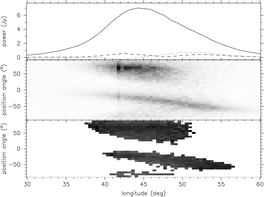
Figure 1: Polarisation-angle-density diagram for PSR B0809+74 at 328 MHz. The top panel gives the usual average Stokes parameters: total power $I$ (solid line); average linear power $L$ (=$\sqrt{Q^{2}+U^{2}}$), corrected for the statistical bias (dashed curve); and average circularly polarized power $V$ (dotted curve). The usual box showing the resolution and off-pulse noise rms level has not been plotted because it would be almost invisible. The central panel displays (in grey scale) the polarization position-angle distibution, where the values in each pixel are weighted properly by the square of their S/N level (see text). Note the two distinct “tracks” corresponding to the two orthogonal polarization modes (separated by about 90^∘). A sequence of length 3600 pulses was used. The bottom panel shows (again in gray scale) the fractional linear polarization distribution for those samples falling above a five standard-deviation noise threshold and weighted as in the central panel. The peak of the distribution is some 60%.

We can see this general behavior in all of these pulsars which have received adequate investigation: B0031$-$07 exhibits low linear polarization and PA “flips” below 1 GHz [Gould & Lyne (1998); hereafter GL]; in PSR B0809+74 we see a similar behavior (Manchester 1971; Lyne et al.  1971); 0820+02 seems to show two “flips” at 408 MHz (GL); 1923+04 has a single “flip” (Hankins et al.  2001); and in 2016+28, perhaps the best studied of all the ${\bf S}_{\rm d}$ pulsars, we see consistent modal dominance effects near the center of its profile (e.g., see GL). For 2016+28 the polarization histograms in Backer & Rankin (1980) and Stinebring et al.  (1984)—see their figs. 18 and 31, respectively—leave no doubt about the characteristics of this overall modal behavior. Studies of pulsar B0943+10 give a detailed, completely consistent example of the situation wherein one mode is consistently stronger than the other (Suleymanova et al.  1998; Deshpande & Rankin 2001). We also see this situation clearly documented in PSR B2303+30 (Backer & Rankin 1980), and GL and Hankins et al. ’s work on 1540+06, 1612+07, 1923+04, 1940$-$12, 2110+27, and 2303+30 reveals compatible behavior. Indeed, that 1923+04 exhibits both behaviors (modal “flips” in some observations and not in others) suggests that modal power variations are probably common in ${\bf S}_{\rm d}$ stars, where they are often comparable in intensity—and slight changes in their relative amplitude would produce different average polarization effects.

3 Observations and analysis

Our 328-MHz observation of PSR B0809+74 was conducted with the Westerbork Synthesis Radio Telescope (WSRT), using its pulsar backend, PuMa. WSRT is an east-west array with fourteen equatorially mounted 25-m dishes. For this observation (which was made on the 26th November 2000), the delays between the dishes were compensated, and the signals were added ‘in phase’ to construct an equivalent 94-m single dish having a sensitivity of about 1.2 K Jy^-1. We also calibrated the telescope array for polarisation measurements following the procedure given by Weiler (1973) and Weiler & Raymond (1976; 1977). With a bandwidth of 10 MHz, centred around 328 MHz, the signals were Nyquist-sampled, and Fourier transformed to synthesize a filterbank of 64 complex frequency channels. Stokes parameters were computed on-line in this frequency domain. Finally, after some averaging, 2-bit (4-level) data samples were recorded for all Stokes parameters and frequency channels, with a time resolution of 819.2 $\mu$sec. During the offline analysis, we removed the interstellar-despersion delay between the signals of various frequency channels, producing multi-bit, floating-point sample values. For this purpose, we used a dispersion measure (DM) of 5.7513$\pm$0.0002 pc cm^-3 as determined by Popov et al. (1987).

Figure 2: Polarisation-angle histogram for PSR B0809+74 at 1365 MHz. The top panel gives the usual average Stokes parameters: total power $I$ (solid line); linear power $L$ (=$\sqrt{Q^{2}+U^{2}}$) (dashed curve); and circularly polarized power $V$ (dotted curve). A box showing the resolution and off-pulse noise rms level is just visible at the left of the diagram. The lower panel represents the histogram of sample position angles with estimated errors less than 30^∘ (see text), together with the superposed average PA traverse. Note the two distict “tracks” corresponding to the two orthogonal polarization modes (separated by about 90^∘). A 2708-pulse sequence was used.

Figure 3: PA histogram for PSR B2303+30 as in Fig. 2. Again, note the two well separated modal PA “tracks”. The display used 2370 pulses and a polarization-angle threshold of 8^∘.

The 1380-MHz observations were also conducted with the WSRT with its pulsar backend, PuMa. All the Stokes parameters were recorded as mentioned above, with a bandwidth of 80 MHz and 512 frequency channels.

The 430-MHz observation of PSR B2303+30 was recorded at Arecibo on 15 October 1992, using the 40-MHz correlator, which “dumped” the ACF/CCF’s of the right- and left-handed channel voltages at 1206 $\mu$sec intervals. Using 10-MHz bandwidth and retaining 32 lags, dispersion delays were reduced to negligible values. The time resolution was then about 0.^∘276 longitude (one rotation period equals 360^∘ longitude). After 3-level correction, the ACF/CCFs were calibrated and Fourier transformed to produce Stokes parameters, which were then corrected for dispersion delays, Faraday rotation, and feed effects (see Suleymanova et al. 1998).

Figures 1 & 2 (at 328 and 1385 MHz, respectively) represent the first available polarization PA “histograms” for pulsar B0809+74. The top panels in these two figures show the usual average polarization properties: total power (Stokes parameter $I$; solid curve), linear power, corrected for the statistical bias (dashed curve), and circular power ($V$; dotted curve). The middle panel of Fig. 1 and the bottom panel of Fig. 2 then give the PA distribution information: in the former as a grey scale with the values contributing to each pixel carefully weighted in order to maximize their significance; and in the latter as a display of sample values comprising a “density plot”. In the first figure, the values contributing to a pixel were weighted according the square of their S/N values—after taking care to estimate the PA error according to the procedure given in Rankin & Rathnasree (1997; see footnote 11); whereas in the latter the PA values are given as “dots” corresponding to all data samples for which the error in the PA, $\sigma_{\chi}$ ($=\sigma_{\rm on}/L$) was less than 30^∘. The on-pulse noise level $\sigma_{\rm on}$ was estimated as $\sigma_{\rm off}(I_{\rm sys}+L)/I_{\rm sys}$, where $I_{\rm sys}$ is the total power corresponding to the system temperature and $\sigma_{\rm off}$ is the standard deviation of the noise in Stokes parameter $I$ well away from the pulse window. (Clearly, $\sigma_{\rm off}/I_{\rm sys}=(2\tau\Delta\nu)^{-{1\over 2}}$, where $\Delta\nu$ is the total bandwidth and $\tau$ the effective integration time.). Finally, the bottom panel of Fig. 1 gives the density of the fractional linear polarization, also as a grey scale—where a fully black pixel represents a value of about 60%. Here, in addition to S/N weighting as above, a threshold of 5 $\sigma_{\rm on}$ was imposed to improve the quality of the display. This detailed analysis and display was possible for the 328-MHz sequence, because the average S/N was relatively high, but was not practical for the other two sequences. A display similar to Fig. 2 for pulsar B2303+30 can be seen in Figure 3.

For both these pulsars the two parallel tracks—corresponding to the two orthogonal modes, separated by about 90^∘—can be very clearly seen. For PSR B0809+74 at the lower frequency, the two modes have comparable power throughout much of the pulse, resulting in severe depolarization; whereas at the higher frequency we see little secondary-mode (herafter SPM) emission during the first half of the pulse, so that most of the depolarization occurs after the peak of the average profile. We can also see here that the PA-traverse rate associated with this SPM emission is -2${}^{\circ}/^{\circ}$ or steeper, a fact that cannot readily be determined from the usual average polarimetry (e.g., the otherwise very well measured profiles recently of GL) as well as one having considerable importance for future efforts to understand the configuration of this pulsar’s rotating subbeam system. These PA “tracks” can now be assessed and interpreted according to the RVM of Radhakrishnan & Cooke (1969)—and the initial evidence here is that they are nearly, but not precisely, orthogonal.

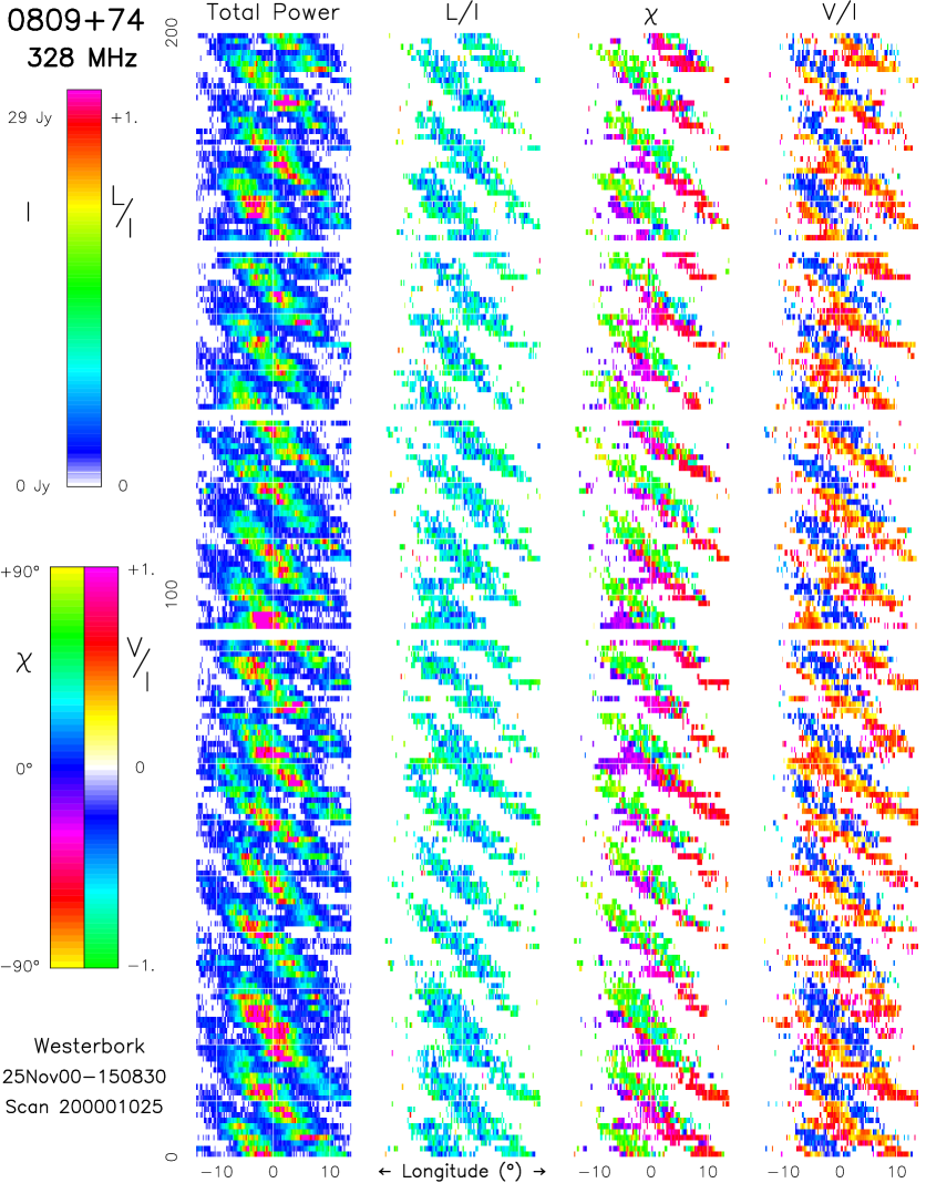
Figure 4: Color display of a 200-pulse portion of the 328-MHz observation in Fig. 1. The first column of the displays gives the total intensity (Stokes parameter $I$), with the vertical axis representing the pulse number and the horizontal axis pulse longitude, colour-coded according to the left-hand scale of the top bar to the left of the displays. The second and third columns give the corresponding fractional linear polarisation ($L/I=\sqrt{Q^{2}+U^{2}}/I$) and its angle ($\chi={1\over 2}\tan^{-1}{U/Q}$), according to the scales at the top-right and bottom-left of the left-most panel. The last column gives the fractional circular polarisation ($V/I$), according to the scale at the bottom-right of the left-hand panel. Plotted values have met a threshold corresponding to 2.5 standard deviations of the off-pulse noise level. Note the strikingly modal character of the polarized power, with the linear assuming nearly orthogonal angles—color-coded as either chartreuse or magneta—and with the corresponding circular falling at about 40% negative (purple) and positive (orange), respectively. It is also notable that the PAs exhibit (apart from noise variations) virtually only these angle values, so that with a single pulse or subpulse, we see not primarily rotation, but modal 90^∘ “flips”. Can it be any wonder that polarization behavior of such remarkable complexity caused so much early confusion?

We further note that while the PA histograms clearly exhibit the modal nature of the polarized power in pulsars 0809+74 and 2303+30, these distributions remain remarkably complex. The widths of the primary polarization-mode (hereafter PPM) and SPM distributions is very different. When the two modal contributions have about equal power, some of the radiation will be randomly polarised (as can be clearly seen in the figures); whereas, when one dominates the other, its PA determines the ensemble PA. Statistical theory discussions of this phenomenon are rather complex (see Davenport & Root 1958; Moran 1976; and especially McKinnon & Stinebring 1998).

Finally, the color polarization display in Figure 4 provides a completely different way of looking at the polarization characteristics of the subpulses. The four columns give the total power, fractional linear polarization (corrected for statistical bias), polarization angle, and fractional circular polarization of the first 200 pulses of the 328-MHz sequence of Fig. 1—all color-coded according to the respective color scales at the far left of the display. Immediately, we see the drift bands—with the individual subpulses drifting from left to right (the pulses are numbered from the bottom to top), the three intervals of “null” pulses, and the fairly consistent, about 40% level of fractional linear polarization. More arresting, however, are the associated polarization angle and circular-polarization behavior, where we find two strongly preferred values for both the PAs—nearly orthogonal values coded chartreuse and magenta, respectively, and respective 40% negative and positive fractional circular values, coded purple and orange.

Careful inspection of the pulse-sequence PA behavior in the figure shows that there are very frequent 90^∘“flips”—usually from about -20^∘ (magenta) to +70^∘ (chartreuse)—but no good example of systematic rotation. Of course, we see variations which may be partly modal and partly the effect of the noise, but were the pulsar subpulses are strongest (e.g., between number 18 and 27) the modal “flips” are clearly seen in every pulse. We do see the longitude of these “flips” occuring at progressively earlier phases, so as to remain approximately parallel to the drift-band and thus within the subpulses as they “drift”—and it was a smeared out signature of this phenomenon which Taylor et al.  recorded 30 years ago.

The full story is, however, much more complex: there is a progressive mixing of the two polarization modes as the subpulses drift across the profile “window”—as subpulses at the extreme edges tend to exhibit only one of the modes. In this context, the constancy of the fractional linear polarization is striking; indeed, one gets the impression that most of individual samples are not modally depolarized—only the contrasting (dark blue) ones which usually lie close to the PA “flips”. Also intriguing is the circular, which is highly correlated with the modal linear power, while exhibiting a slightly displaced distribution along the drift bands. We will return to these questions in much more detail in subsequent papers on 0809+74.

4 Discussion

Polarisation position-angle displays for PSRs B0809+74 and PSR B2303+30, computed from well measured sequences and given above, show clearly that the PAs trace out two well defined, nearly parallel trajectories (separated by approximately 90^∘) as a function of longitude. As such, they individually trace curves which are completely compatible (within their errors) with the Radhakrishnan & Cooke (1969) RVM, and thus entirely exclude the large ($\sim 90^{\circ}$), extraordinary, subpulse-related PA rotations previously reported for these two stars. If such systematic rotations occurred, the character of the distributions would have to be very different—and the Taylor et al.  result—about 90^∘ PA rotation across subpulses occurring over a subpulse-width-order interval of longitude is completely explained by the the prominent, stongly longitude-segregated regions of modal power, together with their subpulse-width-order instrumental resolution. Of course, we can say nothing about any small extraordinary PA rotation within the respective PPM and SPM “tracks”—but this question is well beyond the limited scope of our paper.

Nonetheless, we also see here that the character of the modal emission is exceedingly complex, entailing at least four factors: a) its overall angular and/or temporal distribution—probably following from its generation within a rotating subbeam system, b) our viewing geometry, which determines the manner in which the profile “window” weights the various contributions, and c) the level of instrumental noise. The PA distributions for PSR B0809+74’s two modes at 328 MHz, for instance, are quite different; the PPM’s PA width is much broader than the SPM and their separation may not be just 90^∘. For all these reasons the depolarization in this pulsar is very complex, such that the individual pulse polarization—which is typically 40% linear and circular—is reduced in their aggregation to hardly 5 and 10%, respectively.

Consequently, it should perhaps neither be surprising that PSR B0809+74’s subpulses appeared to exhibit the extraordinary “PA rotation” on the basis of early observational and analytical methods, nor that it has taken fully 30 years to discern that this interpretation was incorrect. Thus, we now hope and trust that this truer, more universal characterization of the pulsar’s polarized emission will facilitate broader and more comprehensive physical explanations of its overall nature.

- (1) Backer, D. C., Rankin, J. M. 1980, ApJS, 42, 143.
- (2) Clark, R. R., Smith, F. G. 1969, Nature 221, 724.
- (3) Davenport, W. B., Root, W. L. 1958, “Random signals and noise” (New York: McGraw Hill)
- (4) Deshpande, A. A., Rankin, J. M. 2001, MNRAS 322, 488.
- (5) Gil, J. A. 1992, A&A 256, 495.
- (6) Gould, D. M., Lyne, A. G. 1998, MNRAS 301, 253.
- (7) Hankins, T. H., Rankin, J. M. & Eilek, J. A. 2001, preprint.
- (8) Komesaroff, M. M. 1970, Nature, 225, 612
- (9) Lyne, A. G., Smith, F., Graham, D. 1971, MNRAS 153, 337.
- (10) Manchester, R. N. 1971, ApJS, 23, 283.
- (11) Manchester, R. N., Taylor, J. H., Huguenin, G. R. 1975, ApJ 196, 83.
- (12) McKinnon, M. M., Stinebring, D. R. 1998, ApJ, 502, 883
- (13) Moran, J. M. 1976, Meth. Exp. Physics, 12C, 228
- (14) Popov, M. V., Smirnova, T. V., Soglasnov, V. A. 1987, Sov. Astr., 31, 529
- (15) Radhakrishnan, V., Cooke, D. J. 1969, ApLett, 3, 225
- (16) Rankin, J. M. 1986, ApJ, 301, 901.
- (17) Rankin, J. M. 1993, ApJS, 85, 145
- (18) Rankin, J. M. & Rathnasree, N. 1997, JAA, 18, 91
- (19) Stinebring, D. R., Cordes, J. M., Rankin, J. M., Weisberg, J. M., Boriakoff, V. 1984, ApJS, 55, 247.
- (20) Suleymanova, S. A., Izvekova, V. A., Rankin, J. M., Rathnasree, N. 1998, JAA 19, 1.
- (21) Taylor, J. H., Huguenin, G. R., Hirsch, R. M., Manchester, R. M. 1971, ApLett 9, 205.
- (22) Weiler, K. W. 1973, A&A, 26, 403
- (23) Weiler, K. W., Raimond, E. 1976, A&A, 52, 397
- (24) Weiler, K. W., Raimond, E. 1977, A&A, 54, 965