The Angular Clustering of Galaxy Pairs

Abstract

We identify close pairs of galaxies from $278\,\rm deg^{2}$ of Sloan Digital Sky Survey commissioning imaging data. The pairs are drawn from a sample of 330,041 galaxies with $18<r^{*}<20$. We determine the angular correlation function of galaxy pairs, and find it to be stronger than the correlation function of single galaxies by a factor of $2.9\pm 0.4$. The two correlation functions have the same logarithmic slope of 0.77. We invert Limber’s equation to estimate the three-dimensional correlation functions; we find clustering lengths of $r_{0}=4.2\pm 0.4\,h^{-1}$ Mpc for galaxies and $7.8\pm 0.7~{}h^{-1}$ Mpc for galaxy pairs. These results agree well with the global richness dependence of the correlation functions of galaxy systems.

1 Introduction

Clusters are observed to be more strongly clustered than galaxies (Bahcall & Soneira 1983; Bahcall 1988; Postman et al. 1992; Croft et al. 1997; Abadi et al. 1998). Moreover, the clustering strength of groups and clusters has been shown to increase with richness (Bahcall & Soneira 1983, Szalay & Schramm 1985, Bahcall & West 1992). Groups of galaxies have a smaller correlation length than that of rich clusters (Merchán et al. 2000) but larger than that of individual galaxies (Connolly et al. 1998, Loveday et al. 1996, Infante & Pritchet 1995). A number of authors have examined the correlation function of groups of galaxies from relatively shallow redshift surveys (Jing & Zhang 1988; Maia & da Costa 1990; Ramella et al. 1990; Trasarti-Battistoni et al. 1997; Girardi, Boschin & da Costa 2000; Merchán, Maia, & Lambas 2000), finding that the groups exhibit a correlation function somewhat stronger than that of galaxies. The richness dependence of the correlation function is generally explained in terms of high-density peak biasing of the galaxy systems (Kaiser 1984), and is seen in cosmological simulations (e.g. , Bahcall & Cen 1992, Colberg et al.  2000 and references therein).

This paper quantifies the angular clustering of pairs of galaxies, thus exploring the dependence of clustering on system richness in the regime between single galaxies and groups. In future work, as an appropriately large sample becomes available, we will investigate the clustering of groups of galaxies (see also Lee & Tucker 2001).

The Sloan Digital Sky Survey (SDSS; York et al. 2000) commissioning data (Stoughton et al. 2001) provide a photometrically reliable catalog of galaxies over a large field to $r^{*}$ $\approx 22.0$. We define a uniform sample of compact galaxy pairs from these data over an area of $278\,\rm deg^{2}$. Scranton et al. (2001) show that systematic effects on galaxy clustering due to star-galaxy separation, varying seeing, photometric calibration, reddening, and so on, are small in these data. The resulting galaxy clustering analysis is presented by Connolly et al. (2001), Tegmark et al. (2001), Szalay et al. (2001), and Dodelson et al. (2001). In the present paper, we extend these results by comparing the angular correlation function of galaxies to that of galaxy pairs. Our magnitude slice samples galaxies with a median redshift of roughly 0.22, appreciably deeper than that of previous group studies.

Assuming an appropriate redshift distribution, we invert Limber’s equation to determine correlation lengths for both galaxies and pairs, and its dependence on the number density of these systems.

In § 2 we describe the Sloan Digital Sky Survey imaging data, the properties of the galaxy catalog, and the definition of galaxy pairs. Estimation of the angular correlation function of galaxies and of pairs is presented in § 3. In § 4 we invert the angular function to determine the spatial correlation scales of galaxies and pairs. The dependence of the correlation scale on richness is presented in § 5, and we give our conclusions in § 6.

2 The Sloan Digital Sky Survey Imaging Survey

The Sloan Digital Sky Survey is a photometric and spectroscopic survey of 1/4 of the sky, above Galactic latitude of $\sim\rm 30^{\circ}$ (York et al. 2000). The photometric data are taken with a dedicated 2.5 m altitude-azimuth telescope at Apache Point, New Mexico, with a $\rm 2.5^{\circ}$ wide distortion-free field and an imaging camera consisting of a mosaic of 30 imaging 2048$\times$2048 SITe CCDs with $\rm 0.4^{\prime\prime}$ pixels (Gunn et al. 1998). The CCDs are arranged in six columns of five CCDs each, using five broad-band filters ($u$, $g$, $r$, $i$ and $z$). The total integration time per filter is 54.1 seconds. Each column of CCDs observes a scanline on the sky roughly $13^{\prime}$ wide; the six scanlines of a given observation make up a strip, and two interleaved strips give a stripe $2.5^{\circ}$ wide. The measured survey depth at which repeat scans show 95% reproducibility is 22.0, 22.2, 22.2, 21.3, and 20.5 magnitudes for the 5 filters, respectively. The SDSS photometric system is measured in the $\rm AB_{\nu}$ system (Oke & Gunn 1983, Fukugita et al. 1996).

Several aspects of the SDSS photometric pipeline (Lupton et al. 2001) are worthy of mention in the context of studies of pairs and groups of galaxies. We use Petrosian (1976) magnitudes, as described by Blanton et al. (2001), Yasuda et al. (2001), and Stoughton et al. (2001). Overlapping images are deblended consistently in five colors, using an algorithm which makes no assumption regarding profile shape or symmetry thereof, and which works with an arbitrary number of overlapping objects. Visual inspection shows that the morphologies and photometry of overlapping galaxies are correctly determined for pairs of objects of similar brightness whose centers are separated by as little as 3 arcsec.

Star-galaxy separation is accurate at the 99% level to at least $r^{*}=20.5$, and better than 90% for $r^{*}\leq 22$ (for $\leq 1.5^{\prime\prime}$ seeing); we discuss this further below. The data are deep enough that the typical photometric error in the Petrosian magnitude of an $r^{*}=20.8$ galaxy is 0.05 mag, plus 0.03 magnitude error to be added in quadrature due to uncertainties in the overall photometric calibration.

2.1 The Data

We use imaging data taken during the commissioning period of the SDSS (on 21 and 22 March 1999), which together make up a stripe $2.5^{\circ}$ wide and $100^{\circ}$ long centered on the Celestial Equator (runs 752 and 756); these data are included in the SDSS Early Data Release (Stoughton et al. 2001). These runs lie within the area $7^{h}.7<{\rm R.A.}\,(2000)<16^{h}.8$ and $-1^{\circ}.26<{\rm Dec.}\,(2000)<1^{\circ}.26$, although the two strips overlap for only the central part of this right ascension range. The seeing ranged from $1.2^{\prime\prime}$ to $2.5^{\prime\prime}$.

For each of the six scanlines of the two runs, we use the data that is more than $30^{\prime\prime}$ from the edge of the CCDs. We carried out tests of the robustness of the derived angular correlation function to the masking of bright stars, and found it to be insensitive to the masking; in what follows, we do not mask the stars. We carry out the pair counts on each of the twelve scanlines separately, normalizing in each one, and then average the results. Note that this differs from the approach of Scranton et al. (2001), who analyze the twelve scanlines together; they also define a mask which excludes bright stars and regions of particularly poor seeing. We will see below that our angular correlation function is essentially identical to theirs. The resulting sample has an effective area of $278.13\,\rm deg^{2}$.

The turnover in the galaxy number counts as a function of magnitude (Yasuda et al. 2001) provides a good estimate of completeness. The galaxy number counts in $r^{*}$ rise as $d\log N/dm\approx 0.4$ up to $R<25$ (Infante, Pritchet, & Quintana 1986; Tyson 1988). Thus any turnover relative to this power law at $r^{*}<25$ can be attributed to incompleteness. Figure 1 shows the galaxy counts for our sample, after correcting for reddening using the extinction maps of Schlegel, Finkbeiner, & Davis (1998) (see Yasuda et al. 2001 for a thorough discussion of the SDSS galaxy counts). The thin solid lines represent the counts for each of the 12 scanlines analyzed. The solid dots are the overall counts for the sample. The bold solid line is the best power law fit to the data points. The slope of the counts is $d\log N/dm=0.46$. The counts begin to turn over noticeably fainter than $r^{*}=20.5$ (although Scranton et al. 2001 show that one can push star-galaxy separation fainter for galaxy clustering analyses). We therefore take our galaxy catalog to be complete to $r^{*}$ $\leq 20.5$.

2.2 The Catalogs

The next step is to generate catalogs of galaxies and galaxy pairs.

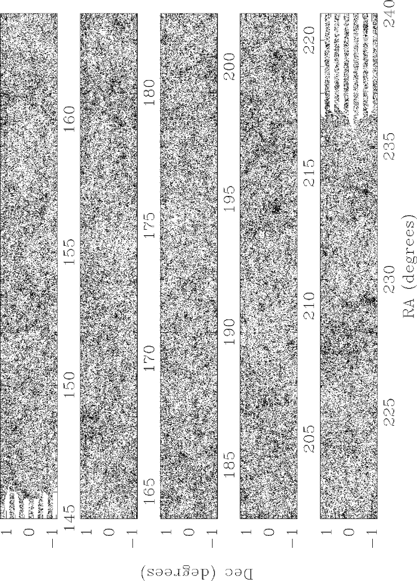
Figure 2: Distribution on the sky of galaxies from runs 752 and 756 with $18<r^{*}<20$. The region shown is centered on the right ascension range over which the two runs overlap.

We wish to work in a fairly narrow magnitude range to minimize redshift projection effects. We also want to avoid problems with completeness, and work in a range where the redshift distribution of galaxies is well-understood (see below). With this in mind, we define a sample in the range $18\leq r^{*}\leq 20$, after correction for reddening as above; this includes $330,041$ galaxies over an area of $278.13\,\rm deg^{2}$. The distribution on the sky of the galaxies in our sample is shown in Figure 2, which shows the region centered on the right ascension range in which the two strips overlap. Although these data are drawn from 12 separate scanlines, the scanline boundaries are invisible where they overlap.

The reliability of the catalog depends on photometric uniformity, the performance of the object deblender, the number of spurious detections around bright stars and edge effects. These issues are discussed by Scranton et al. (2001) and Lupton et al. (2001). In brief, overlaps between adjacent scanlines show photometric zero-point offsets of less than 0.03 mag; similar conclusions are reached from the agreement in galaxy counts between the scanlines as shown in Figure 1. Visual examination of pairs and triplets of galaxies found in the sample (as described below) shows that the deblender works well in over 95% of close pairs. Similarly, examination of regions around bright stars shows essentially no spurious objects in the magnitude range we use. Finally, the overlap between scanlines (roughly $1^{\prime}$) means that, for galaxies smaller than $20^{\prime\prime}$ (which includes essentially all galaxies in our sample), we can reject objects which overlap the edges of the CCDs without leaving any gaps.

We turn now to describe our criteria for selecting isolated galaxy pairs. The galaxy angular correlation function, $\omega(\theta)$, quantifies the ratio of clustered to unclustered systems; we thus work at separations where $\omega(\theta)>1$, to ensure that the excess of pairs over a random distribution is more than a factor of two (see Infante, de Mello, & Menanteau 1996 and Carlberg, Pritchet, & Infante 1994 for further discussion).

The SDSS galaxy redshift survey (cf. Zehavi et al. 2001, Stoughton et al. 2001) extends only to $r^{*}=17.77$, so we use the luminosity function of the CNOC2 redshift survey by Lin et al. (1999) to determine the expected redshift distribution of the sample. We carried out transformations of the photometric bands, following Fukugita et al. (1996), for each galaxy type (see Dodelson et al. 2001 for further discussion of this point). The predicted redshift distribution of galaxies, $dN/dz$, in the range $18\leq r^{*}\leq 20$ is plotted in Figure 3, and of course is consistent with the distributions shown by Dodelson et al. (2001). The predicted median redshift is $\langle z\rangle=0.22$ with a dispersion of $0.09$. In what follows, we explicitly assume that the luminosity function of galaxies in pairs is the same as that of isolated galaxies.

We select groups of galaxies as follows; below, we will limit our analysis to those groups which have exactly two members. We examine all galaxies in the catalog, and find all galaxies within an angular separation of $\theta=15^{\prime\prime}$ (in practice, we also require $\theta>2^{\prime\prime}$, as the deblender rarely separates objects reliably at closer separation). $15^{\prime\prime}$ corresponds to $37\,h^{-1}$ kpc at the median redshift of the sample. We then merge all groups which have members in common. For each group, we define the group radius, R_G, as the angular radius of the smallest circle containing the centers of the group members (for pairs, R_G is half the separation of the two galaxies), and R_N, as the distance from the group centroid to the next galaxy not in the group. Our sample of isolated groups is defined by the criterion R_N/R${}_{G}\geq 3$, which is based on those used for local samples (Karachentsev 1972; Hickson 1982; Prandoni et al. 1994), who show that this decreases the fraction of chance projections in group-finding. We note however that our isolation criterion does not consider galaxies fainter than the sample limit of $r^{*}=20$; in contrast, the low-redshift samples referenced above considered all galaxies up to three magnitudes fainter than the brightest member. We will show below that this makes little difference in our analysis.

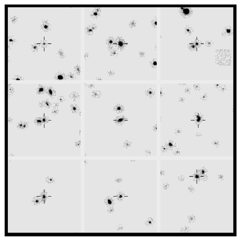
Figure 4: Examples of galaxy pairs in $r^{*}$ . The cross-hair marks one of the members. Each panel is $1.34\times 1.34~{}\rm arcmin^{2}$. These images include foreground stars as well, and are recreated from the SDSS “Atlas Images”, postage stamps extracted around each detected object. Thus there is no background sky noise beyond the boundary of each object.

This sample contains 15,492 close pairs, but only 1175 groups with three or more members, too small a sample to measure a robust correlation function. We therefore carry out the clustering analysis only on the pairs. We inspected the images of a large number of these pairs. Fewer than 3% are spurious detections, e.g. improperly deblended bright extended objects or bright star spikes, meteor trails, etc.. Fig. 4 shows some examples of galaxy pairs from our sample.

In Table 1 we present the main characteristics of the galaxy and pair catalogs. We explicitly assume that the luminosity function, and thus the redshift distribution of galaxies in pairs is the same as that of field galaxies. We list the mean redshift and effective width of the $dN/dz$ distribution. The effective volume, weighted by $dN/dz$, is listed for the samples (equation 6). The correlation statistics are described below.

3 The Angular Correlation Function of Galaxies and Pairs

We determine the angular correlation function of galaxies and of pairs of galaxies using a catalog of randomly distributed points over the survey area, and using the estimator suggested by Landy & Szalay (1993):

$$\omega(\theta)={{N_{dd}-2~{}N_{dr}+N_{rr}}\over{N_{rr}}}.$$ (1)

Here $N_{dd}$ is the number of galaxy pairs in a given range of separations summed over all SDSS fields, $N_{dr}$ is the number of galaxy-random pairs, and $N_{rr}$ is the number of random pairs. Pair counts were done in each scanline separately. The random pair counts were obtained from 100 random catalogs, with galaxies randomly distributed within the net survey area. Random counts were normalized to each scanline separately. We also calculated the correlation function using the method of Infante (1994); the results are indistinguishable.

The resulting angular correlation functions of galaxies and galaxy pairs are shown in Figure 5 and Table 1. The error bars result from 100 bootstrap re-sampling variations; these conservative errors (see the discussion in Fisher et al. 1994) are somewhat larger than the scatter from one scanline to another, presented for the galaxy pair sample in Figure 6. The galaxy angular correlation function follows a power law, $\omega=A_{\omega}\theta^{(1-\gamma)}$, with $\gamma=1.77\pm 0.04$, and an amplitude essentially identical with that given by Connolly et al. (2001), when their results for the $18<r^{*}<19$ and $19<r^{*}<20$ slices are combined. In agreement with the latter paper, we find no breaks in the correlation function on scales smaller than one degree.

The galaxy pair correlation function shows the same power law behavior as the galaxies, but with a significantly larger amplitude.

The error bars determined by the bootstrap resampling method in the galaxy correlations are smaller than the symbols. Scranton et al. (2001) discuss the angular correlation and the related uncertainties in greater detail; our results are consistent with theirs. We have also carried out a jack-knife estimation of the errors, and find consistent results with those presented here.

We fit each of the correlation functions to a power law; the results are given in Table 1. These fits use the bootstrap errors, but unlike Connolly et al. (2001) do not take the covariance into account; we may therefore be underestimating our error bars on $r_{0}$ somewhat.

Our galaxy pair sample is defined without redshifts, over a fairly narrow range of apparent magnitude. This could give rise to two types of systematic error in the estimated clustering strength. First, distant clusters of galaxies might have only two members bright enough to enter the galaxy sample, and therefore could masquerade as a galaxy pair; as clusters exhibit appreciably stronger clustering than do groups (e.g., Bahcall 1988), this could bias the results. However, at $z\sim 0.22$, the density of galaxy pairs is much higher than the density of clusters. Thus, any contamination from background clusters should be small. To check this, we searched for galaxies as faint as $r^{*}=21.5$ around each pair, and found no significant density enhancements. Thus there is no evidence that many of our pairs are the “tips of the iceberg” of distant clusters.

Second, inclusion of pairs in projection will tend to systematically decrease the clustering amplitude. We have carried out simulations of the effects of random projection on the clustering of our pair catalog. We find that of order $f=30\%$ of our pairs are likely to be chance projections along the line of sight. The angular correlation function is depressed by a factor $(1-f)^{2}$ by projection; this suggests that the correlation amplitude of groups listed in Table 1 should be multiplied by a factor of order two.

4 The Three-Dimensional Correlation Function of Galaxies and Pairs

We relate our $\omega(\theta)$ measurements to the three-dimensional correlation functions $\xi(r)$ via Limber’s Equation (Limber 1953). The spatial correlation function is assumed to be a power law weighted by the standard phenomenological evolutionary factor, $\xi(r,z)=\left({r}\over{r_{0}}\right)^{-\gamma}(1+z)^{-(3+\epsilon)}$, where $r$ is the proper distance, $r_{0}$ is the proper correlation length, and $\epsilon$ is the clustering evolution index. $\epsilon=\gamma-3$ corresponds to clustering fixed in comoving coordinates, while $\epsilon=0$ represents stable clustering in physical coordinates (Phillips et al. 1978).

Parameterizing the angular clustering as $\omega(\theta)=A_{\omega}\theta^{(1-\gamma)}$, $r_{0}$ is given by

$$r_{0}^{\gamma}=A_{\omega}^{-1}~{}C~{}{{\int_{0}^{\infty}g(z)(dN/dz)^{2}dz}\over{[\int_{0}^{\infty}(dN/dz)dz]^{2}}}$$ (2)

(e.g. Efstathiou et al. 1991; see also Peebles 1980 and Phillips et al. 1978). $C$ is a constant involving purely numerical factors,

$$C=\pi^{1/2}~{}{{\Gamma[(\gamma-1)/2]}\over{\Gamma(\gamma/2)}}$$ (3)

and the function $g(z)$ depends only on $\epsilon$, $\gamma$, and cosmology:

$$g(z)=\left({dz}\over{dx}\right)x^{1-\gamma}F(x)(1+z)^{-(3+\epsilon-\gamma)}$$ (4)

where $x(z)$ is the coordinate distance and $F(x)$ is

$$F(x)=[1-(H_{0}a_{0}x/c)^{2}(\Omega_{0}-1)]^{1/2}.$$ (5)

We use a cosmology with $q_{0}=0.1$ and $\Lambda=0$, and an evolution index of $\epsilon=0$ as suggested by observations (Carlberg et al. 2000).

The $H_{0}$ dependence of $g(z)$ is canceled by that in the measured value of $r_{0}$. The strong dependence of $A_{\omega}$ on $dN/dz$ is clear in this equation. Note in particular that the above equations are not affected by galaxy evolution, except in the calculation of the redshift distribution $dN/dz$ (Peebles 1980, eqs. [56.7] and [56.13]). However, Limber’s equation, as presented here, does assume that galaxy clustering is independent of luminosity; the high-redshift objects in our narrow magnitude slice are of higher luminosity than the low-redshift objects. Clustering is in fact weakly dependent on luminosity (e.g., Norberg et al. 2001 and references therein), but the quantification of this effect on our results is beyond the scope of this paper.

Because our sample covers a narrow magnitude range, and the galaxies in pairs have essentially the same mean magnitude as the entire galaxy sample (Table 1), we expect the $dN/dz$ of pairs to be identical to that of galaxies (Figure 3). This allows us to estimate the correlation lengths, $r_{0}$, for the clustering of galaxies and pairs. We find that pairs have a significantly larger correlation length than do galaxies; $r_{0}=4.2\pm 0.4$ $h^{-1}~{}\rm Mpc$ for galaxies and $7.8\pm 0.7h^{-1}~{}\rm Mpc$ for pairs. These values are to be compared with $\sim 5$ $h^{-1}~{}\rm Mpc$ for galaxies (Davis & Peebles 1983; Loveday et al. 1996, Infante & Pritchet 1995), $\sim 7-8$ $h^{-1}~{}\rm Mpc$ for groups (Carlberg et al. 2001, Girardi et al. 2000, Merchán et al. 2000) and $\sim 15-20$ $h^{-1}~{}\rm Mpc$ for rich clusters (Bahcall & West 1992). The errors in our derived $r_{0}$ include both statistical uncertainty, as well as an uncertainty added in quadrature due to our imperfect knowledge of the redshift distribution (cf., the discussion by Dodelson et al. 2001).

In the following section, we will relate the clustering length to the mean inter-system separation of galaxies and groups. We determine the latter from the effective volume of the sample, based on the model redshift distribution:

$$V={{\int_{z_{min}}^{z_{max}}(dN/dz)V(z)dz}\over{\int_{z_{min}}^{z_{max}}(dN/dz)dz}}$$ (6)

which then yields the number density, $n={N_{systems}\over{V}}$, and mean separation, $d=\left({1}\over{n}\right)^{1/3}$. We find the mean separation of galaxies and galaxy pairs is 3.7 and 10.2 $h^{-1}$ Mpc, respectively. Note that random superpositions will artificially depress the pairs value of $d$ by a factor $(1-f)^{1/3}\approx 0.9$; thus the true value of $d$ for pairs is probably closer to $11\,h^{-1}$ Mpc.

5 The $r_{0}~{}-~{}d$ Relation

The correlation lengths of galaxies and galaxy pairs are compared with the global richness-dependent correlations of galaxy systems (Bahcall & Soneira 1983, Szalay & Schramm 1985, Bahcall 1988) in Fig. 7. Here the correlation scales $r_{0}$ of various systems are plotted as a function of the mean separation of the objects, $d$; since richer systems are rarer, the quantity $d$ scales with the richness or mass of the systems. The data points include groups and clusters of galaxies of different richnesses and different samples: rich Abell clusters (Bahcall & Soneira 1983, Peacock & West 1992, Postman et al. 1992, Lee & Park 2000; note that Richness 0 clusters cannot be included in any statistical analyses since they are no complete samples of these objects); APM clusters (Croft et al. 1997 (C97); Lee & Park 2000 (LP00); the latter find considerably larger $r_{0}$ in their re-analysis of the APM clusters); EDCC clusters (Nichol et al. 1992): X-ray selected clusters (REFLEX survey, Böhringer et al. 2001; XBACS survey, Abadi et al. 1998, Lee & Park 2000); and groups of galaxies (Merchán et al. 2000; Girardi et al. 2000). The well-known dependence of $r_{0}$ on $d$ (Bahcall 1988, Bahcall & West 1992) is clearly observed. The new result presented for pairs of galaxies, with $d=10.2~{}h^{-1}$ Mpc and $r_{0}=7.8\pm 0.7~{}h^{-1}$ Mpc, fits well within this universal clustering trend; it is significantly larger than the galaxy correlation scale, and somewhat smaller than the correlation scales observed for small groups of galaxies.

Also presented in Fig. 7 is the expected $r_{0}~{}-~{}d$ relation for two cosmological models: LCDM ($\Omega_{m}=0.3$, $\Omega_{L}=0.7$, $h=0.7$) and Standard CDM (SCDM; $\Omega_{m}=1$, $h=0.5$) (both models are normalized to the present-day cluster abundance). These relations are obtained from large scale, high resolution cosmological simulations (Governato et al. 2000; Colberg et al. 2000; Bahcall et al. 2001). Figure 7 highlights the fact that the SCDM model is highly inconsistent with the clustering data – not only for rich clusters, as was previously known (e.g., Bahcall & Cen 1992, Croft et al. 1997, Governato et al. 2000, Colberg et al. 2000) – but also for small groups and galaxy pairs; the correlation strength observed for all these systems is systematically stronger than predicted by SCDM models. The LCDM model provides a considerably better match to the data; the lower the value of $\Omega_{m}$, the stronger the group correlations predicted. This ‘canonical’ model is consistent with most other observations of large scale structure, clusters of galaxies, supernovae Ia, and the cosmic microwave fluctuations (e.g. , Bahcall et al. 1999, Wang et al. 2000). In fact, the data may even suggest a somewhat lower $\Omega_{m}$ than 0.3, as some of the best data points exhibit stronger correlations than expected for $\Omega_{m}=0.3$.

Note that the lower $r_{0}$ values for the two richest (but small) sub-samples of APM clusters are due to their exceptionally steep correlation function slope: $\gamma\sim-3$ instead of $\sim-2$; all other sample have a slope of $\sim-2$. This steepness reduces $r_{0}$, bringing it lower than the other relevant data.

6 Conclusions

We use a sample of 330,041 galaxies within a stripe of area 278 deg² centered on the Celestial Equator, with magnitudes $18\leq r^{*}\leq 20$, obtained from SDSS commissioning imaging data. We use these data to select isolated pairs of galaxies. We determine the angular correlation function of the galaxies and of the galaxy pairs. We find the following results:

• Pairs of galaxies are more strongly clustered than are single galaxies. The angular correlation amplitude of galaxy pairs is $2.9\pm 0.4$ times larger than that of galaxies.

• The power-law slopes of the two correlation functions are the same, corresponding to $\gamma=1.77\pm 0.04$.

• We measure $\omega(\theta)$ up to 1 deg scales, corresponding to $\sim 9~{}h^{-1}~{}\rm Mpc$ at the mean redshift of 0.22. No breaks are detected in either correlation function.

• Assuming a redshift distribution from the CNOC2 survey luminosity function, we invert the angular correlations and determine a three-dimensional correlation length, $r_{0}$, for each sample. We find $r_{0}=4.2\pm 0.4$ $h^{-1}~{}\rm Mpc$ for galaxies and $7.8\pm 0.7h^{-1}~{}\rm Mpc$ for pairs; the latter may be biased downward somewhat by projection effects.

• The mean separation between systems is $d=3.7$ and $10.2~{}h^{-1}$ Mpc for galaxies and pairs respectively. The correlation lengths fit the global $r_{0}~{}-~{}d$ relation observed for galaxy systems well (Bahcall & West 1994).

This work suggests a number of follow-up studies. We have defined pairs of galaxies from their positions on the sky, and we need to quantify what fraction of these objects are pairs at the same redshift. We are in the process of carrying out a redshift survey of a subset of the pairs sample, which will also be useful in tying down the $dN/dz$ relation. We can also use photometric redshifts from the multi-band photometry of the SDSS to define a cleaner sample of galaxy pairs. Finally, we have used just under 300 deg² of SDSS data in this study; the survey has now imaged over five times this area. Thus we are in the process of defining samples of richer (and thus rarer) systems from this larger area, and measuring their correlations, to investigate the $r_{0}-d$ relation between for richer groups.

Table 1: Properties of Galaxies and Pairs ($18\leq r^{*}\leq 20$)

Property	Galaxies	Pairs
Mean redshift $\langle z\rangle$	$0.22\pm 0.1$	$0.22\pm 0.1$
Effective Volume [$h^{-3}~{}\rm Mpc^{3}$]	$17.8\times 10^{6}$	$17.8\times 10^{6}$
$\langle r^{*}\rangle$ [SDSS band]	19.34	19.30
Number	330,041	15,492
$A_{\omega}$, ($\gamma$)	$4.94\pm 0.02$ (1.77)	$13.54\pm 0.07$ (1.76)
Correlation length $r_{0}~{}[h^{-1}~{}\rm Mpc]$	$4.2\pm 0.4$	$7.8\pm 0.7$
Mean spacing $d\ [h^{-1}~{}\rm Mpc]$	3.7	$10.2$

Note. — $H_{0}=100h\rm\,km\,s^{-1}\,Mpc^{-1}$, $q_{0}=0.1$, $\Lambda=0$, $\epsilon=0$;

Area covered: $278.13~{}\rm deg^{2}$

Figure 1: $r^{*}$ differential galaxy number counts. The data are the number of galaxies per magnitude per deg². The thin solid lines represent the counts of 12 individual scanlines. The solid circles are the overall number counts in the total $278.13\,\rm deg^{2}$. The bold solid line is a power law fit to the data. The line can be represented as ${\log(N\,\rm mag\,\rm deg^{2})}=0.46r^{*}-6.03$. The galaxy sample is complete to $r^{*}=20.5$.

Figure 3: Normalized redshift distribution of galaxies in the range $18\leq r^{*}\leq 20$ based on luminosity functions from the CNOC2 redshift survey (Lin et al. 1999). The median redshift is $\langle z\rangle=0.22$, with a FWHM of $0.09$.

Figure 5: Angular correlation function of galaxies and galaxy pairs for $18\leq r^{*}\leq 20$. The x-axis is separation in arcsec, measured on a logarithmic scale on the lower axis, and a linear scale on the upper axis. The open points are the measured galaxy correlation function, and the solid points are the measured pair correlation function. The thin solid line is the fit to the Connolly et al. (2001) correlation function with $\gamma=1.73$, scaled to our magnitude range. The dashed line is the best fit model for galaxies, with $r_{0}=4.2~{}h^{-1}$ Mpc. The dot-dashed line is the best fit model for pairs with $r_{0}=7.8~{}h^{-1}$ Mpc. The error bars are determined by bootstrap resampling, and are smaller than the symbol size for the galaxies.

Figure 6: Angular correlation function of galaxy pairs for each scanline separately. The solid line is the fit to the SDSS galaxy correlation function from Connolly et al. (2001), scaled to our magnitude range.

Figure 7: Correlation length $r_{0}$ versus mean separation $d\,(=n^{-1/3})$ for galaxies and pairs, as well as groups and clusters of galaxies (see § 5, which describes the different samples plotted). The predictions from simulations of two cosmological models, LCDM and SCDM, are shown for comparison, as well as the original approximate relation of $r_{0}~{}\approx~{}0.4~{}d$ for rich systems (Bahcall 1988).

References

- (1) Abadi, M.G., Lambas, D.G., & Muriel, H. 1998, ApJ, 507, 526
- (2) Bahcall, N.A. 1988, ARA&A, 26, 631
- (3) Bahcall, N.A., & Cen, R. 1992, ApJ, 309, L81
- (4) Bahcall, N.A., Ostriker, J.P., Perlmutter, S., & Steinhardt, P.J. 1999, Science, 284, 1481
- (5) Bahcall, N.A., & Soneira, R.M. 1983, ApJ, 270, 20
- (6) Bahcall, N.A., & West, M.J. 1992, ApJ, 392, 419
- (7) Bahcall, N.A., et al. 2001, in preparation
- (8) Blanton, M. et al. 2001, AJ, 121, 2358
- (9) Böhringer, H. et al. 2001, A&A. 369, 826
- (10) Carlberg, R., Pritchet, C., & Infante, L. 1994, ApJ, 435, 540
- Carlberg et al. (2000) Carlberg, R. G., Yee, H. K. C., Morris, S. L., Lin, H., Hall, P. B., Patton, D., Sawicki, M., & Shepherd, C. W. 2000, ApJ, 542, 57
- (12) Carlberg, R., Yee, H.K., Morris, S.L., Lin, H., Hall, P.B., Patton, D.R., Sawicki, M. & Shepherd, C.W. 2001, ApJ, 552, 427
- (13) Colberg, J.M. et al. 2000, MNRAS, 319, 209
- (14) Connolly, A.J., Szalay, A.S., & Brunner, R.J. 1998, ApJ, 499, L125
- (15) Connolly, A.J. et al. 2001, AJ, submitted (astro-ph/0107417)
- (16) Croft, R.A.C, Dalton, G.B., Efstathiou, G., Sutherland, W.J., & Maddox, S.J. 1997, MNRAS, 291, 305
- (17) Davis, M., & Peebles, P. J. E. 1983, ApJ, 267, 465
- (18) Dodelson, S. et al. 2001, ApJ, submitted (astro-ph/0107421)
- (19) Fisher, K. B., Davis, M., Strauss, M. A., Yahil, A., & Huchra, J. P. 1994, MNRAS, 266, 50
- (20) Fukugita, M., Ichikawa, T., Gunn, J.E., Doi, M., Shimasaku, K., & Schneider, D.P. 1996, AJ, 111, 1748
- (21) Girardi, M., Boschin, W., & da Costa, L.N. 2000, A&A, 353, 57
- (22) Governato, F., Babul. A., Quinn, T., Tozzi, P., Baugh, C.M., Katz, N. & Lake, G., 1999, MNRAS, 307, 949
- (23) Gunn, J.E., Carr, M.A., Rockosi, C., et al. 1998, AJ, 116, 3040
- (24) Hickson, P. 1982, ApJ, 255, 382
- (25) Infante, L. 1994, A&A, 282, 353
- (26) Infante, L., de Mello, D.F., & Menanteau, F. 1996, ApJ, 469, L85
- (27) Infante, L. & Pritchet, C. 1995, ApJ, 439, 565
- (28) Infante, L., Pritchet, C., & Quintana, H. 1986, AJ, 91, 217
- (29) Jing, Y., & Zhang, J. 1988, A&A, 190, L21
- (30) Karachentsev, I.. 1972, Comm. Spec. Astrophys. Obs., 7, 1
- (31) Kaiser, N. 1984, ApJ, 284, L9
- (32) Landy, S.D. & Szalay, A.S. 1993, ApJ, 412, 64
- (33) Lee, S., & Park, C. 2000, ApJ, submitted (astro-ph/9909008)
- (34) Lee, B., & Tucker, D. 2001, in The New Era of Wide Field Astronomy, edited by R. Clowes, A. Adamson, and G. Bromage, ASP Conference Series # 232, 170
- (35) Limber, D. N. 1953, ApJ, 117, 134
- (36) Lin H., Yee., H.K.C., Carlberg, R.G., Morris, S.L., Sawicki, M., Patton, D.R., Wirth, G., & Shepherd, C.W. 1999, ApJ, 516, 552
- (37) Loveday, J., Efstathiou, G., Maddox, S.J., & Peterson, B.A. 1996, ApJ, 468, L1
- (38) Lumsden, S.L., Nichol, R.C., Collins, C.A., & Guzzo, L. 1992, MNRAS, 258, L1
- (39) Lupton, R.H. et al. 2001, in preparation
- (40) Maia, M.A.G. & da Costa, N.L. 1990, ApJ, 349, 477
- (41) Merchán, M.E., Maia, M.A.G., & Lambas, D.G. 2000, ApJ, 545, 26
- (42) Nichol, R., Collins, C., Guzzo, L. & Lumsden, S.L., 1992, MNRAS, 255, L21
- (43) Norberg, P. et al. 2001, MNRAS, 328, 64
- (44) Oke, J.B., & Gunn, J.E. 1983, ApJ, 266, 713
- (45) Peacock, J.A., & West, M.J. 1992, MNRAS, 259, 494
- (46) Peebles, P.J.E. 1980, “The Large Scale Structure in The Universe” (Princeton: Princeton University Press)
- (47) Petrosian, V. 1976, ApJ, 209, L1
- (48) Phillips, S., Fong, R., Fall, R.S., Ellis, S.M., & MacGillivray, H.T. 1978, MNRAS, 182, 673
- (49) Postman, M., Huchra, J.P., & Geller, M.J. 1992, ApJ, 384, 404
- (50) Prandoni, I., Iovino, A., & MacGillivray, H.T. 1994, AJ, 107, 1235
- (51) Ramella, M., Geller, M.J., & Huchra, J.P. 1990, ApJ, 353, 51
- (52) Schlegel, D., Finkbeiner, D., & Davis, M. 1998, ApJ, 500, 525
- (53) Scranton, R. et al. 2001, ApJ, submitted (astro-ph/0107416)
- (54) Stoughton, J. et al. 2001, AJ, submitted
- (55) Szalay, A.S., & Schramm, D.N. 1985, Nature, 314, 718
- (56) Szalay, A.S. et al. 2001, ApJ, submitted (astro-ph/0107419)
- (57) Tegmark, M. et al. 2001, ApJ, submitted (astro-ph/0107418)
- (58) Trasarti-Battistoni, R., Invernizzi, G., & Bonometto, S.A. 1997, ApJ, 475, 1
- (59) Tyson, J.A. 1988, AJ, 96, 1
- (60) Wang, L., Caldwell, R.R., Ostriker, J.P., & Steinhardt, P.J. 2000, ApJ, 530, 17
- (61) Yasuda, N. et al. 2001, AJ, 122, 1104
- (62) York, D.G. et al. 2000, AJ, 120, 1588
- (63) Zehavi, I. et al. 2001, ApJ, submitted (astro-ph/0106476)