Variability of accretion flow in the core of the Seyfert galaxy NGC 4151

Abstract

We analyze observations of the Seyfert galaxy NGC 4151 covering 90 years in the optical band and 27 years in the 2 - 10 keV X-ray band. We compute the Normalized Power Spectrum Density (NPSD), the Structure Function (SF) and the Autocorrelation Function (ACF) for these data. The results show that the optical and X-ray variability properties are significantly different. X-ray variations are predominantly in the timescale range of 5 - 1000 days. The optical variations have also a short timescale component which may be related to X-ray variability but the dominant effect is the long timescale variability, with timescales longer than $\sim 10$ years. We compare our results with observations of NGC 5548 and Cyg X-1. We conclude that the long timescale variability may be caused by radiation pressure instability in the accretion disk, although the observed timescale in NGC 4151 is by a factor of few longer than expected. X-ray variability of this source is very similar to what is observed in Cyg X-1 but scaled with the mass of the black hole, which suggests that the radiation pressure instability does not affect considerably the X-ray production.

1 Introduction

NGC 4151 ($z=0.00332$; $D=13.2$ Mpc assuming Hubble constant 75 km s^-1 Mpc^-1) is one of the classical Seyfert 1 galaxies. It is among the most frequently observed AGN and therefore it is an excellent object for variability studies, although it is both typical and atypical representative of its class, as nicely and extensively summarized by Ulrich (2000). We therefore chose it as a second source (after NGC 5548; Czerny, Schwarzenberg-Czerny, & Loska 1999) for which the nature of the variability can be studied by computing the normalized power spectrum density (hereafter NPSD) in both the optical and the X-ray bands.

The host galaxy is a typical spiral galaxy SAB(rs)ab of 11.3 mag brightness in B band (Perez et al. 1998). The extinction due to our Galaxy is low (A${}_{V}<0.01$ in B band) because NGC 4151 is located near the North Galactic Pole ($b_{II}=75.1^{\circ}$). However, the intrinsic extinction in NGC 4151 is considerable: in the optical region, A${}_{V}=1^{m}.0$ in BLR and A${}_{V}=0^{m}.7$ in NLR (Ward et al. 1987). Direct estimates in the UV bands give much less extinction (E${}_{B-V}=0.06$) for wavelength $\lambda 2200$ Å  corresponding to A${}_{V}=0^{m}.18$ (Wu & Weedman 1978). The hydrogen column density inferred from the equivalent widths of ultraviolet absorption CIII lines is about $1.7\times 10^{19}$ cm^-2 (Kriss et al. 1992), smaller than the inferred X-ray column density. The X-ray observations clearly indicate that the nuclear X-ray continuum is significantly obscured, by an equivalent hydrogen column $N_{H}=(1-10)\times 10^{22}$ cm^-2) (Yaqoob et al. 1993), which would correspond to A${}_{V}\approx 5^{m}-50^{m}$ according to the standard relation between A_V and N_H from Reina & Tarenghi (1973).

HST observations suggested that the line of sight towards the nucleus (at least in the epoch when the observation was performed, on 1991 June 18/19) lies outside the ionization cone (Evans et al. 1993). However, broad emission lines - which can vary in strength - are usually easily detected, although with superimposed absorption features (e.g. Brandt et al. 2001); only during one observation, in 1984, the broad component of H_β was absent (Lyutyj, Oknyanskij & Chuvaev 1984; Penston & Pérez 1984; see also Pronik, Sergeev, & Sergeeva 2001) and the spectrum more closely resembled that of a narrow emission line or a Seyfert 2 type galaxy. Therefore it seems that most of time the nucleus is viewed directly and the scattered component characteristic for Seyfert 2 galaxies does not dominate the spectrum, apart from the soft X-ray band (see Ogle et al. 2000).

Regardless of the fact that X-ray extinction is high, the intrinsic X-ray spectrum seems to be fairly typical for a Seyfert galaxy (Zdziarski, Johnson, & Magdziarz 1996). The brightness of the nucleus varies dramatically on all timescales in all energy bands. Spectrum and variability in the 50 - 150 keV band was studied by Johnson et al. (1997); the source shows a factor of 2 variability in days and years. The X ray (2 - 10 keV) variability of this source was studied in more detail using Fourier analysis, starting with the paper by Fiore et al. (1989). It was found (Papadakis & McHardy 1995) that X-ray variability power spectrum of NGC 4151 covering the range $10^{-6}-10^{-8}$ Hz can be described by a power law, which is significantly flatter than that measured on short time scales ($10^{-2}-10^{-5}$ Hz) derived from EXOSAT observations. The power law index measured by Hayashida et al. (1998) on the basis of the Ginga data in the frequency region of $10^{-4}-10^{-6}$ Hz has an index $\alpha=2.1$.

The long-term optical variability of the continuum in the UBV band was studied by Lyuty & Doroshenko (1999). They showed that a long photometric minimum in years 1984 - 1989 separates two active phases: 1968 - 1988 (Cycle $\cal A$) and 1989 - 2000 (Cycle $\cal B$). The decrease of brightness continued in 2000 and at the end of 2000, the brightness of the variable component reached almost the same level as in 1987 - 1988 (Doroshenko et al. 2001). These phases are also seen in the JHKL-bands (Lyutyi, Taranova, & Shenavrin 1998).

The power spectrum density (PSD) of the NGC 4151 optical flux variations in 1968 - 1987 was studied by Terebizh, Terebizh, & Biryukov (1989). It was found that the PSD in the frequency range $10^{-4}-2\times 10^{-2}$ day^-1 (time interval from 50 days to 30 years) corresponds to flicker noise with slope $\approx$ 1 in logarithmic scales and the light curve may be interpreted as a result of superposition of flares randomly distributed in time. The behavior of the structure function (hereafter SF), focusing on the intra-night variability and conducted between 1989 - 1996 was studied by Merkulova, Metik & Pronik (2001). Collier & Peterson (2001), using the same technique, determined the characteristic timescale to be $13^{+11}_{-5}$ days.

Long timescale trends in optical variability of NGC 4151 were studied by Lyutyj & Oknyanskij (1987) and Fan & Su (1999), on the basis of data covering the period from 1910. Lyutyj & Oknyanskij (1987) noted the quasi-periodic changes with typical time of 4 and 14 years. Also Fan & Su (1999) claimed the presence of the periodicity, with the period 14.0 $\pm$ 0.8 yr, during which both the brightness and the spectral type changed. It is not surprising that both groups found the similar quasi-periodical processes in optical light curve because the main data set used by both teams was the same. Some earlier papers also claimed the presence of the periodic variability albeit with other values of the period (e.g. Pacholczyk (1971) found a period of 5.1 years), while other papers argued against any strict periodicity (e.g. Pacholczyk et al. 1983; Terebizh et al. 1989).

The short term multiwavelength variability was best studied by AGN Watch team and was summarized by Edelson et al. (1996). They concluded that significant and correlated variability was observed in the X-ray, UV and optical bands, with phase differences consistent with zero lag and normalized variability amplitude decreasing with increasing wavelength. They calculated the power spectrum in the UV on timescales of $\approx$ 0.2 - 5 days and showed that the power spectrum is falling down rapidly at short timescales and the bulk of the variability power is on timescales of days or longer.

In the present paper we reanalyze the optical and X-ray data available in the literature which cover respectively 90 and 25 years. Such a broad dynamical range allows us to draw conclusions about the character of the accretion flow and the possible nature of the instabilities responsible for the observed variability.

2 Observational data

2.1 Optical band

The observational data in optical region used in the present paper come from different sources. Long data sets were collected by the team at the Crimean Station of the Sternberg Astronomical Institute (1968 - 2000), the Special Astrophysical Observatory in the Caucasus (1997 - 2000), and the Maidanak Observatory of the Ulugbek Astronomical Institute in Uzbekistan (1990 - 2000). Below, we will refer to these data as the Crimean data. The data collected in the three bands (U, B, and V) cover the period from 1968 till 2000. The data points are not distributed uniformly since the source was at some seasons unobservable at the sites involved. Nonetheless, the sets consist of about 1150 points in each color, thus providing an exceptionally long and well sampled light curve for any AGN. The light curve and the discussion of the variability amplitude and color changes were presented by Lyuty & Doroshenko (1999) and Doroshenko et al. (2001). Additionally, shorter data set (about 300 points during 1989 - 1999) in the infrared band R is also available (Doroshenko et al. 2001).

Shorter, but more densely spaced data set was taken from the AGN Watch team (Kaspi et al. 1996). Those data cover only 98 days but they add 62 points to the long set. Continuum flux in the spectral band 4560 - 4640 Å was fitted to the flux in the B-band of Crimean data set using regression relation based on 17 common dates of observations.

The majority of the oldest data points was derived by Pacholczyk et al. (1983) from the old Harvard and Stewart Observatories photographic plates. These data cover the period from 1910 until 1968. Besides those observations we used data from Fitch, Pacholczyk, & Weymann (1967), Cannon, Penston, & Brett (1971), Penston et al. (1971), and Oknyanskij (1978; 1983). Comparison of the photographic magnitudes between various data sets and with Crimean photoelectric data in B-band for overlapping dates of observations allowed us to reduce the photographic data into photoelectric B-bands magnitudes.

As a result, in the B-band we obtained a quite long data set covering years 1910 - 2000. We must note that the similar work of gathering all photographic observations was made by Lyuty and Oknyanskij (1987), but in comparison with this work we added more photoelectric observations made after 1984. A subsequent compilation of the 1910 - 1991 data was prepared by Longo et al. (1996) but they used even older data from heterogeneous sources and interpolated the data in order to obtain equally spaced data points which lead to large errors so finally they had to ignore the first 30 years of observations.

The full combined light curve of the NGC 4151 nucleus in the B band is shown in Fig. 1. Open circles mark the historical photographic plate data while the Crimean data are shown with the continuous line. A small expanded fraction of the light curve from JD2449150 till JD2449550 is inserted in that Figure. It includes the three month period when the dense AGN Watch data were collected. Crimean data are shown with continuous line and the AGN Watch points are marked with crosses. The figure demonstrates that the variability in 1910 - 1978 based on photographic data is similar in its character to the variability in 1968 - 1989 covered by photoelectric observations. Also the AGN Watch data agrees well with the corresponding fragment of the Crimean observations: the AGN Watch data points are located on the quasi-linear part of the light curve showing local rise in brightness. Therefore, we consider the old data as generally reliable.

The overall character of the variability is not constant over the entire data set - the behavior of the optical light curve in 1990 - 2000 appears different from that in 1910 - 1985. The evolution up to 1985 can be represented by a single parabolic-type curve with maximum flux of about 75 - 80 mJy in B band and with superimposed on it more rapid variations. In 1935 there was (if the photographic magnitudes were estimated correctly) the strongest flare which lasted only 10 - 15 days. A less intense flare happened in 1946 but it is based on a single point. The evolution in 1990 - 2000 appears as a single giant outburst but this change in the character of variability occurred in the middle of the epoch 1968 - 2000 covered by the photoelectric data.

2.2 X-ray data

The data in the 2 - 10 keV X-ray band also came from different papers and databases which were collected using different satellites. Fluxes were corrected for absorption. The observed time coverage is from October 1974.

The data points during 1975 - 1992 were taken from Papadakis & McHardy (1995). Of their 133 data points, a majority came from the Ariel V Sky Survey, and others were taken from literature including observations by EXOSAT, GINGA, OSO-8, HEAO-1, TENMA and Ariel VI satellites. Some additional points (in period May 1987 - May 1995) were taken from Yaqoob & Warwick (1991) and Yaqoob et al. (1993) and were also taken from the Tartarus Database of ASCA observations . We corrected their fluxes for absorption using the HEASARC’s online W3PIMMS Version 3.1 flux converter as well as papers of Weaver et al. (1994) and Edelson et al. (1996). Data from the first three years of RXTE observations during October 1998 – November 1999 were taken from Markowitz & Edelson (2001). The observational data given in that paper in $counts/s$ were transformed into unabsorbed fluxes via the mean luminosity of $300$-day window given in the paper. We supplemented those gathered data with three long sequences. Two EXOSAT light curves were obtained from Ian M. McHardy for the paper by Czerny & Lehto (1997). These data cover 10 and 11 July 1983 and 15 May 1985, with rate sampling every $100$ s. Third sequence, from the ASCA satellite, covers the period from 12 till 23 May 2000, and is nearly continuous (except for Earth occultations and the passages through the South Atlantic Anomaly). For that ASCA data set, we use the count rate sampling of 32 s. The measurements in $counts/s$ were again converted to fluxes using the mean luminosity for an appropriate data sequence.

All daily-averaged X-ray points used by us for further analysis are shown in Fig. 2 with open circles.

Figure 1: The light curve of NGC 4151 in the B band from the historical plate data (open circles connected with a continuous line) and Crimean observations (solid line). Inserted expanded fragment shows the AGN Watch data (crosses) together with Crimean data (continuous line). The errors are on the order of 0.2 mag ($\sim 20$ %) for the historical plate data and $\sim 1.5$ % for the Crimean observations.

Figure 2: The light curve of NGC 4151 ($\nu F_{\nu}$) in U band (solid line) and in X-ray band (2 - 10 keV absorption-corrected flux, open circles). The errors of X-ray data are on the order of a factor 2 in the oldest data points and of $\sim 10$ % for more recent measurements. The errors in Crimean data are $\sim 2.2$ %.

3 Methods

3.1 Power spectrum

We attempt the restoration of the underlying power spectrum $|F|^{2}$ of the active nucleus from its observed light curves, i.e. from the product of the true light curve and the sampling (window) function. Direct analysis of observations yields the observed power spectrum $|G|^{2}$, i.e. the underlying spectrum affected by the window function $|W|^{2}$. These functions obey an exact relation in the Fourier transform space:

$$G=F*W$$ (1)

where $*$ denotes the convolution and $F$, $G$ and $W$ are Fourier transforms of the underlying and observed light curves and of the sampling function. For long and nearly uniformly sampled observations $|W|^{2}$ approaches the delta function and $G$ approximates $F$. For non-uniform sampling, the shape of the window function becomes complex, with broad wings and many local maxima. In such case it is difficult to obtain a solution of Eq. (1) for $F$ as it involves deconvolution of the sampling transform $W$.

We address the issue of uneven sampling by not calculating the power spectrum of the entire light curve directly. Instead, we analyze the properties in various time scale ranges separately.

In the optical band, we first rebin the data to 1 yr bins and fill the few existing gaps by linear interpolation, thus obtaining 90 data points. Next we rebin the original curve into 5 day bins and find an almost continuous sequence containing 2403 such points. Data gaps are again filled through interpolation. We calculate the power spectra of the two sequences separately and combine them by averaging the logarithmic values.

In the X-ray band, we also first rebin the data to 1 yr bins (25 points). Next we rebin the original light curve into 30 day bins and find and almost continuous fragment (26 points). Next we rebin the original data into 5 day bins obtaining 69 points in an almost continuous set. Finally, the two light curves from EXOSAT and one from the ASCA monitoring were rebinned to 4096 s bins. The power spectra of the resulting six light curves were computed independently and combined for further analysis.

For uniformity, all optical data points are converted from magnitudes to flux units, when necessary, and the average value is subtracted. The NPSD of each light curve is computed according to the description by Hayashida et al. (1998):

$$NPSD(f)={1\over\overline{x(t)}^{2}}a(f)a^{*}(f)\times T,$$ (2)

with

$$a(f)={1\over n}\sum_{i=1}^{n}{x(t_{i})\exp(2\pi ift_{i})},$$ (3)

where $x(t_{i})$ is the value of the flux at the time $t_{i}$, $T$ is the length of the data set and $\overline{x(t)}$ is the mean value of the flux. Therefore, the integrated NPSD gives half of the fractional variance.

The errors of the power spectra obtained as above are either estimated directly from the data or estimated using the Monte Carlo simulations (see Appendix A).

Table 1: The basic parameters of the variability.

Color	band	Flux (mJy)	rms (mJy)	$F_{var}$	$R_{max}$	error
Whole data
U,B,V (1968-2000), R (1989-2000), X-ray (1975-2001), Btot (1910-2000)
X-ray	[2-10] keV	2.55e-2∗	1.07e-2∗	0.41	37.4	10.0%
U	3600 Å	48.44	24.25	0.50	8.7	2.5%
B	4400 Å	63.56	21.09	0.33	3.9	1.5%
Btot	4400 Å	63.23	19.17	0.32	5.2
V	5500 Å	92.26	19.45	0.21	2.6	1.0%
R	7000 Å	169.84	30.78	0.18	2.5	2.0%
Cycle $\cal A$ (25.03.1968 - 03.07.1988)
U	3600 Å	31.88	10.66	0.33		2.5 %
B	4400 Å	48.26	9.10	0.18		1.5 %
V	5500 Å	77.82	8.37	0.11		1.0 %
Cycle $\cal B$ (11.02.1989 - 13.03.2000)
U	3600 Å	63.51	23.32	0.37		1.3 %
B	4400 Å	75.35	20.09	0.27		0.74%
V	5500 Å	103.43	18.18	0.18		0.83 %

$F_{var}$ - rms to mean ratio, $R_{max}$ - maximum to minimum flux ratio
^∗ Flux at 2 keV computed assuming $\alpha=1$ energy index in 2 - 10 keV band

3.2 Structure function

For the analysis of our time series we also used the structure function technique (SF). The application of SF allows us to study both stationary and nonstationary processes. The SF was introduced by Kolmogorov in 1941 for analysis of the statistical problems connected with turbulence theory (Kolmogorov 1941a; b). In astronomical practice, the wide application of the SF to time-series analysis begun in the middle eighties (e.g. Simonetti, Cordes, & Heeschen 1985; Paltani, Courvoisier, & Walter 1998; Kataoka et al. 2001).

As a rule, most work in astronomy uses only the first-order structure function ($SF_{1}$). By definition the structure function of the first-order is a mean square of difference $[x(t)-x(t+\tau)]$:

$$SF_{1}(\tau)=M[(x(t)-x(t+\tau)]^{2},$$ (4)

where $x(t)$ is random process and $\tau$ is time shift. Since we do not use higher order structure functions, we simply denote $SF_{1}$ as $SF$.

In the case of a stationary random process the $SF$ is directly related to the autocorrelation function:

$$SF(\tau)=2D[x(t)]\times[1-ACF(\tau)],$$ (5)

where D[x(t)] is variance of the process and ACF is the autocorrelation function.

The slope of the $SF$ changes with time interval $\tau$. If the measurement errors are neglected, on the shortest time scale the variability can be well approximated by a linear trend, and then $SF\propto\tau^{2}$. For long time scales, the slope of the $SF$ becomes flatter and in the limit when $\tau\rightarrow\infty$ the structure function saturates: $SF\rightarrow 2D[x(t)]$. The addition of measurement errors to the random process increases $SF$ by the value $2D_{err}$ where $D_{err}$ is the variance of the measurement errors. Therefore, $SF\rightarrow 2D_{err}$ when $\tau\rightarrow 0$.

Many processes are stochastic in nature. For some processes such as fractional Brownian motion, the $SF$ shows a power law dependence on $\tau$. Some processes can be represented as a superposition of a large number of random impulses of deterministic form (shot noise). Sub-group of those processes which are characterized by the $PSD(f)\propto 1/f^{\gamma}$ are called flicker noise. If $\gamma$ takes values from 1 to 3, then in this case the structure function $SF(\tau)\propto\tau^{b}$ where $b$ takes values from 0 to 2, following the relation

$$\gamma=b+1.$$ (6)

The structure function analysis was done using a software package by S.G. Sergeev from the Crimean Astrophysical Observatory. The whole time interval was divided into equal bins in logarithmic scale and for each bin we found such pairs of observations with $t_{j}>t_{i}$ that their time difference $\tau_{k}=t_{j}-t_{i}$ fitted into the given bin. Next we calculated the value

$$SF(\tau_{k})=\sum_{i,j}{[x(t_{j})-x(t_{i})]^{2}\over n_{k}},$$ (7)

where $n_{k}$ is the number of pairs in k-th bin. We estimate the errors of the SF as described in the Appendix B.

To allow a meaningful comparison of the SF in various bands we introduce also the normalized structure function (NSF) as follows:

$$NSF(\tau)={SF(\tau)\over D[x(t)]}.$$ (8)

In this case all NSF should approach the universal value 2 on long timescales.

3.3 Autocorrelation function

In our computation of ACF, we again use of program package by S.G. Sergeev; the method used relies on the interpolation. Specifically, for any point from the real data, a corresponding shifted point is found by linear interpolation or extrapolation, and extrapolation is made adapting $x(t>t_{max})=x(t_{max})$ and $x(t<t_{min})=x(t_{min})$ (for a more detailed description, see Sergeev et al. 1999).

4 Results

4.1 General variability properties of NGC 4151

The basic variability properties of the Seyfert galaxy NGC 4151 seen in the data assembled by us are summarized in the upper part of the Table 1. We give there the mean flux at the given spectral band, rms fluctuations, the normalized amplitude $F_{var}$ (i.e. rms to mean ratio) and the ratio $R_{\max}$ of the maximum to the minimum flux. The full 90 years of the B band data are given separately from the data subset determined by photoelectric measurements.

The normalized variability amplitude is the largest in U band and decreases towards the longer wavelengths. This effect is well established for AGN (e.g. Ulrich et al. 1997) and tells us that the variable component is bluer than the non-variable (starlight) component.

The overall normalized variability amplitude in the X-ray band is comparable to the amplitude in U band. However, more extreme variability events occasionally happen in X-ray band while the systematic long timescale dimming/brightening seems to be stronger in U band than in X-rays. The energy content is significantly greater in the variable part of the optical spectrum than in the X-ray spectrum. Variable part of $\nu F_{\nu}$ in U band is equal to $2.02\times 10^{-10}$ erg cm^-2 s^-1 while the variable part of the 2 - 10 keV flux is only $0.81\times 10^{-10}$ erg s^-1 cm^-2. Of course we do not know the bolometric corrections needed for more strict comparison of the total X-ray and optical variable energy output but, they are not likely to reduce this discrepancy considerably. Therefore, we conclude that strong long timescale trends in the optical band do not result from reprocessing of the variable X-ray emission, unless X-ray variability leads to strong variations of the extinction, thus amplifying the effect.

4.2 Stationarity of the data

Question of whether light curves of AGN covering a time span of several decades may be considered realizations of a stationary process is interesting per se, but also because of its possible influence on investigations of variability on shorter time scales (e.g. Leighly 1999, Press & Rybicki 1997). We address this issue by estimating of the importance of any existing linear trend.

4.2.1 Optical band

Even the visual inspection of the light curves of NGC 4151 clearly shows some long timescale trends although they become less prominent with an increase of the data length. It can be best studied in the B band since at that color the available light curve covers the longest time span.

We analyzed the longest trends by rebinning the data in one year bins in order not to be biased by the most recent time spans with superior data coverage as compared with the earliest data from the beginning of the previous century. We studied the trends both using magnitudes (effectively logarithmic scale) or using $\nu F_{\nu}$ fluxes (effectively linear scale).

Mean value of the B magnitude in the Crimean observations is 11.83. Apart from two major outbursts, the presence of the linear trend is also seen in the data. Linear fit in magnitude scale gives a shift by -0.35 mag during the entire period of observations (32 years). This is comparable to the value of the dispersion in this period, calculated for unbinned data (0.33 mag). The result is similar if flux ($\nu F_{\nu}$) is used: linear trend gives the net brightening by $1.2\times 10^{-10}$ erg s^-1 cm^-2, with the dispersion equal $1.4\times 10^{-10}$ erg s^-1 cm^-2. However, if the entire data set of 90 years of data is analyzed, the linear trend acts in the same direction but is much weaker. Systematic shift is only -0.13 mag, or $3.6\times 10^{-11}$ erg s^-1 cm^-2, with the dispersion unchanged.

This shows that the data are not strictly stationary even on the timescale of 90 years. However, in the longest data set the linear trend is much weaker than the typical amplitude of the variability (in B band) and the criterion for stationarity is roughly satisfied. It is less so in the case of shorter sequences, so the power spectra and the structure function may depend on the choice of the data set. This is particularly well known from the studies of X-ray light curves of galactic sources (e.g. Uttley & McHardy 2001, and references therein; for quasar sample see Manners, Almaini, & Lawrence 2001).

4.2.2 X-ray band

X-ray data cover only the period from 1974 till 2000, and the older data (till $~{}\sim 1986$) seem to show larger scatter so the presence or the absence of the long trends is less apparent (see Fig. 2).

We again rebinned the data in one year bins in order to achieve a uniform distribution on long time scales and looked for a linear trend in the resulting light curve. The mean 2 - 10 keV flux was $1.98\times 10^{-10}$ erg s^-1 cm^-2 while the linear trend gave the systematic brightening of the source by $4.12\times 10^{-12}$ erg s^-1 cm^-2, much lower than the dispersion in the data during this period ($8.1\times 10^{-11}$ erg s^-1 cm^-2). Such absence of the linear trend in the data is partially accidental - more accurate Ginga/ASCA/RXTE data (1978 - 2000) cover the period which started and ended up at a very similar level of the activity of the source. Slightly shorter sequences show trends up to almost an order of magnitude stronger but still smaller than the dispersion.

This suggests that the X-ray flux is more likely to be produced by a stationary process during the observed period than the optical flux during the same epoch. Note however, that the time scales used for sampling of the X-ray flux range from seconds up to decades, i.e. have a greater dynamical range than the time scales of optical sampling, which range from days up to nearly a century.

In this context a detection of the change of slope (and in particular, of flattening) of the PSD towards longer time scales might be easier in X-rays than it would be in the optical band. A few more years of occasional monitoring are needed to confirm such a statement.

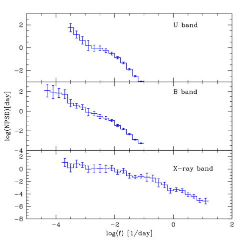
Figure 3: Normalized Power Spectrum Density of NGC 4151. Upper panel: U band (1968 - 2000); middle panel: B band (1910 - 2000); lower panel: X-ray band (1974 - 2000). Marked errors are direct observational errors, as described in Appendix A.

Figure 4: Upper panel: error contours (thick line - 68% confidence level, thin line - 90% confidence level) for the fit of the power law with an index $\alpha$ and a break at $\log f_{0}$ to the NPSD of NGC 4151 in the B band (1910-2000; dashed line) and X-ray band (continuous line) determined from Monte Carlo simulations (see Appendix A). Cross marks the location of the best fit. Intermediate and lower panels show the plots of the marginal probability for both parameters in the X-ray band (continuous line) and in the optical band (dashed line).

4.3 Power spectrum

4.3.1 Optical band

We analyze first the Crimean data alone, covering the years from 1968 till 2000, in all three color bands.

The power spectrum in the U band (see Fig. 3, top panel) has roughly a power law shape with a steep slope ($\sim 2$) but the presence of some structure is clearly visible. A flattening is seen at a timescale of $\sim 300$ d which seems to separate two variability components. No flattening is seen at the longest timescales but the data set used to determine this power spectrum covers only $\sim 10$ years. In the V band, the spectrum (not shown) shows practically no substructure. Given all this, we infer that the interesting timescales are rather long, and therefore concentrate on the results derived from the complete set of data in B band, covering the entire 90 years. The result is shown in Fig. 3, middle panel. In similarity to the U band power spectrum, the B band data show a hint of the presence of two components, separated at the timescale on the order of $\sim 300$ days. The data also reveals the flattening of the low frequency component (roughly at timescale of $\sim 10$ years) although the measurement errors are large.

In order to determine whether the flattening of the power spectrum is real and not simply caused by the finite extension of the data, we performed Monte Carlo simulations assuming that the power spectrum of the entire 90 years of the data in B band is represented by a broken power law model

$$f\propto\left\{\begin{array}[]{ccc}const{}{}{}&{\rm if}~{}~{}~{}\log f<f_{0}\\ f^{-\alpha}&{\rm if}~{}~{}~{}\log f>f_{0}\end{array}\right.$$ (9)

The best fit values of the model parameters are given in Table 2, together with 1 $\sigma$ errors for each parameter. Full two-dimensional contour errors are shown in Fig. 4. Despite the fact that the data used for this cover such an exceptionally long period, the errors are still considerable: the NPSD is consistent with a single power law. It is steeper than 1.5 and the flattening happens at timescales longer than 15 years. We note here that the outlined procedure for computation of the confidence levels is based on likelihood function derived from simulations. Conceptually it is different from the $\chi^{2}$ method employed in Appendix A. The two methods converge only in an asymptotic limit of infinite number of observations. Here we adopt the former method as the more conservative one, yielding much broader confidence limits.

Table 2: The NPSD parameters determined from Monte Carlo simulations for a single break model of 1910-2000 B light curve and two models of the X-ray light curve, one with a single and another with a double break

Band	slope					$\chi^{2}$
Btot	$1.8^{+0.3}_{-0.1}$					5.14/15 dof
X-ray	$1.3^{+0.5}_{-0.1}$					20.16/23 dof
Band	slope	$\log f_{0}[d^{-1}]$	slope			$\chi^{2}$
Btot	0	$-4.3^{+0.8}_{-\infty}$	$1.8^{+\infty}_{-0.3}$			5.14/14 dof
X-ray	0	$-2.1^{+0.5}_{-1.2}$	$1.5^{+0.5}_{-0.2}$			12.39/22 dof
Band	slope	$\log f_{1}[d^{-1}]$	slope	$\log f_{2}[d^{-1}]$	slope	$\chi^{2}$
X	0	$-3.1^{+1.1}_{-\infty}$	1	$-0.7^{+0.6}_{-0.7}$	2	20.31/22 dof

Quoted errors are determined from $\chi^{2}_{dist}$ statistics (see Appendix A) and correspond to 1 $\sigma$ error for one parameter of interest.

We reploted the resulting NPSD in the form of $Power\times Frequency$ diagram (see Fig. 5) in order to better illustrate the dominant time scales. The component corresponding to the timescale of years appears to dominate, but the Figure also shows the presence of a separate, month-timescale component, as well as a possible high frequency roll-over to the last component at about $\log f$(days)$=-2$. It would agree with the characteristic timescale determined by Collier & Peterson (2001).

Lyuty & Doroshenko (1999), analyzing the data from the period 1968 - 2000, argued that there were two cycles of activity in NGC 4151 which differed considerably regarding the level of variability: first one from 1968 till 1988 (cycle $\cal A$) and other from 1989 till the present time (cycle $\cal B$). Since the duration of the outburst $\cal B$ - the dominant feature in the optical light curve (see Fig. 1) - corresponds to the characteristic frequency seen in our analysis, we repeated this analysis for the data set in the B band without the cycle $\cal B$. The NPSD computed without the cycle $\cal B$ still showed a flattening at $\log f$(days)$\sim-3.6$ but above it the NPSD was even better represented by a single power law with a slope $\sim 2$.

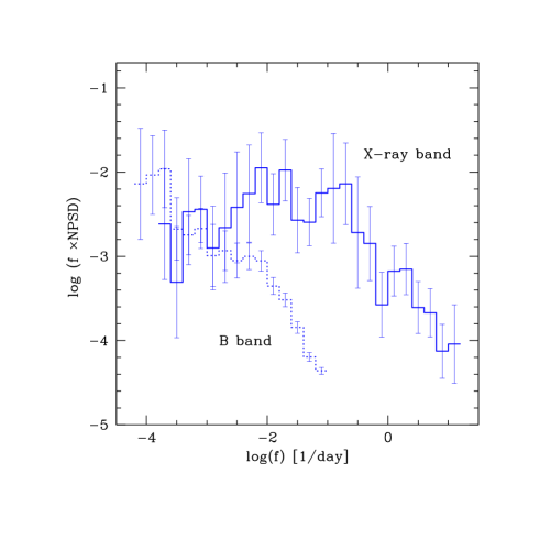
Figure 5: A plot of NPSD multiplied by the frequency, illustrating the frequency regime where most of the power is present: dotted line - B band (1910 - 2000), continuous line - 2 - 10 keV band. Lower panel shows the error contours for the fit of the NPSD with two broken power laws of slopes 0, 1 and 2, and the break frequencies given by $\log f_{1}$ and $\log f_{2}$. Cross marks the best fit position.

4.3.2 X-ray band

X-ray PSD is distinctively different from the optical NPSD (see Fig. 3). Most of the power is now on much shorter timescales. The spectrum generally shows a flattening on time scales of about 100 days, but more structure can be identified. The spectrum might be crudely represented as a broken power law, with slope 1 at intermediate frequencies and about 2 at higher frequencies. The normalization at high frequencies is similar to that obtained by Hayashida et al. (1998). The position of the flattening determined by Papadakis & McHardy (1995) is now in the middle of the intermediate part.

The characteristic features of the shape are again apparent on $Power\times Frequency$ plot (see Fig. 5). Most of the X-ray power is concentrated between $\sim 6$ days and $\sim 150$ days, with a turnover both at higher and lower frequencies. There may also be a decrease in the variability level at the intermediate timescales of $\sim 30$ days. There may also be some additional power at the lowest frequencies but at the lower level than in the optical band.

Since the effect of the specific window function is even stronger for X-ray data than for the optical data, we again performed Monte Carlo simulations, as described in Appendix A. We considered two models for the shape of the NPSD.

The first model was a broken power law identical to the adopted model for the optical power spectrum (see Eq. 9), with the frequency break and the slope above it being the free parameters of the model. The slope obtained from simulations (see Table 2) is slightly flatter than the optical one, but the difference is within 1 $\sigma$ error. However, the best fit break frequency of the NPSD in the X-ray band corresponds to a timescale of around $\sim 100$ days. Formal contour errors slightly overlap (see Fig. 4), particularly at the 90% confidence level but the probability maxima are well separated. The marginal probability plots made by integrating the probability distribution along one of the parameter axis (see the intermediate panel of Fig. 4) show that the distributions of the slopes in the optical and X-ray NPSD are only slightly different, namely they are shifted by $\sim 0.4$ decades, while the distributions of the characteristic variability timescale are essentially different. The value on the order of 100 days is favored for X-ray data but for the optical data the maximum coincides with the longest timescale under study ($\sim 100$ years). It strongly supports the view that the X-ray and optical variability properties at long timescales are significantly different.

The second model was the shape frequently adopted for the galactic sources, a power law distribution with two breaks but fixed slopes of 0, 1 and 2 at the lowest, intermediate and the highest frequencies. Such a model is also a good representation of the observed power spectrum, although formally, the best fit model has a lower acceptance probability than in the previous case. The break frequencies in the best fit model correspond to the timescales of $\sim 6$ days and $\sim 1000$ days. The low frequency break is at lower frequencies than expected from Fig. 5 since apparently the extra power at the lowest frequencies shifts it towards longer timescales.

The spectrum may perhaps be better represented by a number of Lorentzian components, as suggested e.g. by Pottschmidt et al. (2002) for galactic sources but the quality of our light curves was not high enough to attempt more sophisticated fits.

4.4 Structure function

The analysis via the structure function was applied to the Crimean data covering the years from 1968 till to 2000 in UBVR bands, to the combined photographic plus photoelectric data in B band covering the years from 1910 till to 2000, to the AGN Watch data, and also to the X-ray data collected from the literature.

4.4.1 Optical band

Figure 6: The structure function for NGC 4151: upper panel - X-ray band, second panel - U band, third panel - B band (Crimean data - filled circles; AGN Watch - open circles; photographic data - triangles), lowest panel - V band. Errors given here are statistical errors (see Appendix B). Dashed line shows the level of SF due to the measurement error in the data.

Fig. 6 shows SFs for the optical flux in various bands, where the Crimean data is plotted with filled circles. One can see that the shape of the SF which would have been inferred from the Crimean V magnitude data alone can be very well described as a single power law form, with the slope $b\approx 0.7$ for time scale of variability from 1 to 3200 days. Such value of $b$ shows that the dominating process is a single shot noise process. But in the U and B bands, the shape of the SF is more complex, and a clear break in the SF is seen at about 30 - 50 days, with much steeper slope at short timescales and a flatter one in long timescales. The results of Merkulova et al. (2001) show that the steep slope continues down to the timescales of minutes. It can again indicate that in these two time intervals two different processes operate. We therefore measured separately the slope in time interval from 1 to 40 days and in time interval from 80 to 3200 days (see Table 3). Again, in the V band, a single slope of 0.7 provides a good representation of the variability in all timescales shorter than 3200 days (8.8 years) but at shorter wavelengths the two slopes are significantly different. This difference is most visible in U band. The traces of similar structure are only barely seen in V band.

We treated separately the SF of AGN Watch data. Continuum fluxes at $\lambda$ 4600 Å were converted to fluxes in B band and plotted as open circles in the third panel of Fig. 6). The corresponding points match well the Crimean data above the timescales of $\sim 10$ days but they steepen significantly below. This effect is probably due to the presence of a strong linear trend in the optical data during the period covered by AGN Watch monitoring (see Fig. 1). Such a linear trend translates into $SF\propto\tau^{2}$, as can be shown analytically from Eq. 4. This kind of discrepancy underlies the importance of using as long time series of observations as possible in order to avoid artifacts.

One of the important characteristics of the structure function is the point which marks the beginning of plateau at the long time lags. This time scale gives the maximum time scale T_max of correlated signals or, equivalently, the minimum time scale of uncorrelated behavior. From Fig. 6 we can see that the SF reaches plateau at $\log\tau\approx 3.2-3.6$, i.e. about 1600 - 4500 days. We can estimate it most accurately in the B band, due to the longest time coverage in this band. Since the photographic data is of relatively low accuracy, and the number of data points is small in comparison with photoelectric measurements, we compute separately the SF only for historical data. This structure function is shown in the third panel of Fig. 6 with open triangles. We see that the slopes of structure functions derived from both data sets are similar within the errors. Although the length of historical data set is about 25200 days ($\log\tau=4.4$), the plateau begins earlier, at about $\log\tau=3.2$ (corresponding to the time interval 1600 days). So the existence of the plateau is not an artifact of an insufficiently long data train, but its presence is supported by long observations.

The flattening observed in SF at 1600 - 4500 days (4 - 12 years) corresponds well to the flattening hinted by the optical NPSD, at $\sim 10$ years. The change of the slope at some temporal frequency is also seen in both cases, although it does not happen precisely at the same timescales. SF suggests a break at $\sim 30$ while that apparent in the NPSD is at $\sim 500$ days.

Although the SF is less sensitive to the window function problem than the NPSD technique, we performed some Monte Carlo simulations to estimate better the uncertainties involved in the analysis. We adopted a shot noise model of the light curve, with the model parameters

$$dT,\alpha,\beta,T_{min},T_{max};~{}~{}~{}~{}~{}b=2+\alpha+2\beta,$$ (10)

being the mean time separation of the flare, power law index of flare number distribution, power law index of flare duration distribution, minimum and maximum duration of a flare, correspondingly (see Appendix B).

The best fit model parameters representing the Crimean data in the U, B and V bands are given in Table 4), and the best fit models are shown in Fig. 7. There is a good overall agreement between the SF for the best fit model and the SF derived from the data (see lower panel of Fig. 7 for comparison of the observed and modeled SF in V band). The SFs in all three colors are basically similar to each other although hints of systematic differences may be seen at the intermediate timescales between 1 and 60 days, reflecting the minor difference in the best fit parameters. Those differences are marginally significant. In the lower panel of Fig. 7 we show the dispersion of the SF for the family of Monte Carlo curves in the V band; the indicated error is about 0.2 in logarithmic scale at intermediate timescales and becomes larger at long and short timescales.

We also used all the data collected in the B band in order to exploit fully the data length. The result is shown in Fig. 8. In this Figure we plot the normalized structure function for better comparison between various curves, and we also subtract the value $2\sigma_{err}^{2}$, i.e. twice the variance of the measurement uncertainties. On the old photographic data we adopt a measurement error of 8.5%. We see that the SF is not significantly different from the one obtained from the Crimean data alone. However, the apparent flattening of the SF at the longest timescales is still better visible due to the access of the longest timescales.

Figure 7: Upper panel: the structure function in three color bands for the Crimean data (U - continuous line, B - thick dashed line, V - thin dashed line), with the contribution from observational errors subtracted. Lower panel: comparison of the SF for the data (dashed line) and for the best fit model (thick line) in the V band. The error on the simulated SF in the lower panel is determined from the dispersion in Monte Carlo simulations (see Appendix B). Dotted lines show the level of SF due to the measurement error in the data.

Figure 8: Normalized SF for observational data. Upper panel: results for X-ray band with long timescale trends determined from daily averages, and short timescale trends from the ASCA data alone, together with the SF for the cycle $\cal A$ averaged over UBV band. Second panel: comparison of SF averaged over UBV bands for the cycles $\cal A$ and $\cal B$. Third panel: comparison of the result from all combined photographic (ptg) and photoelectric (phe) data in B band with photoelectric Crimean B band data alone. Lowest panel: comparison of the X-ray SF with V band SF based on Crimean data (see Fig. 7) and best fit V band model; the envelope of the V curve marks the error estimate from Monte Carlo simulations.

An interesting question is whether the variability properties during flares are different, and to address this, we repeat our analysis for the two cycles $\cal A$ and $\cal B$ separately. All slopes of the SF are presented in Table 3. An inspection of Table 3 reveals that the properties of the light curves ($SF$ slopes) are significantly different in the two cycles. During the cycle $\cal B$ the slope difference between the short and long timescales is moderate, although a feature around $\sim 50$ days is present. The plateau for long time intervals begins at $\log\tau$=3.2 - 3.4. During the cycle $\cal A$, the difference of the slopes is apparent in all color bands, with the long timescale slope being very flat (Fig. 9; see also Fig 8, second panel), suggesting that long timescale trends are relatively weak. Monte Carlo simulations with short lasting shots (20 days and less) reproduced well the observed light curve properties. This is caused by the fact that in the cycle $\cal A$ we do not see a single large outburst but instead, a number of weaker eruptions superimposed on a weak longer trend. The localization of $T_{max}$, which is the time scale when SF reaches plateau, is less clear in the cycle $\cal A$ than in the cycle $\cal B$, or in the composite data. During the cycle $\cal A$ there are no significant differences in the SF shape for all three UBV colors.

The systematic difference between the cycles is also reflected in our Monte Carlo simulations (see Table 4). We see most clearly a shift (reduction) in the maximum duration of the flares in the best fit model for the cycle $\cal A$ alone in comparison to the model for the whole Crimean data: this reduction is from 800 days to 20 days.

Figure 9: Optical light curve properties during the cycle $\cal A$. Upper panel: the observed light curve in U band and a representative light curve from Monte Carlo simulations, normalized to the mean flux and offset for clarity. Middle panel: observed SF in three color bands. Lower panel: mean and dispersion of the SF from Monte Carlo simulations for best fit model parameters, together with the observed SF in the U band.

Table 3: Structure function slopes b in various color bands, data sets, and timescales.

Band	$b$	$\sigma(b)$	$r$	$b$	$\sigma(b)$	$r$
Cycle $\cal A$ (25.03.1968 - 03.07.1988)
	(1 - 40) days			(80 - 3200) days
U	1.24	0.08	0.95	0.15	0.04	0.61
B	1.15	0.10	0.94	0.18	0.04	0.66
V	1.07	0.10	0.93	0.17	0.04	0.64
mean UBV	1.04	0.08	0.95	0.16	0.03	0.64
Cycle $\cal B$ (11.02.1989 - 13.03.2000)
	(1 - 40) days			(80 - 1500) days
U	1.24	0.05	0.98	0.58	0.04	0.94
B	1.12	0.03	0.99	0.64	0.04	0.96
V	0.86	0.04	0.98	0.67	0.04	0.96
mean UBV	1.02	0.04	0.99	0.63	0.04	0.96
Cycles $\cal A+B$ (25.03.1968 - 13.03.2000)
	(1 - 50) days			(80 - 3200) days
U	1.21	0.08	0.96	0. 60	0.03	0.97
B	1.06	0.06	0.97	0. 64	0.03	0.98
V	0.95	0.05	0.97	0. 66	0.02	0.98
Photographic observations + Cycles $\cal A+B$ (5.03.1910 - 13.03.2000)
	(1 - 40) days			(80 - 3200) days
B	0.99	0.07	0.95	0. 60	0.03	0.98
X-rays (20.10.1974 - 05.01.2000)
	80 min - 10 days			(10 - 4700) days
2-10 keV	1.24	0.04	0.98	0. 23	0.02	0.90

Spectral bands are marked in column (1), time interval for correlated variability are specified above columns (2 – 4) and above columns (5 – 7), slopes $b$ and errors of slope, $\sigma(b)$, are shown in column (2), (3) and (5), (6), and correlation coefficients $r$ for the corresponding linear regressions are in column (4) and (7). Errors of the slopes are determined from fitting the power law to SF points in a specified timescale range.

Table 4: The SF model parameters determined from Monte Carlo simulations.

Cycle	$\cal A$	$\cal{A+B}$
Band	U	U	B	V
dT [days]	0.10	0.20	0.25	0.25
$\beta$	0.45	0.25	0.25	0.17
$\alpha$	-1.47	-1.80	-1.70	-1.60
$T_{min}$ [days]	0.01	0.01	0.01	0.01
$T_{max}$ [days]	20	800	800	800
$\log(\tau)_{min}$	-0.05	0.03	-0.05	0.03
$\log(\tau)_{max}$	1.3	3.0	3.0	3.0
$b$	$1.22$	$0.70$	$0.79$	$0.74$
error $b$ (1$\sigma$)	$\pm 0.17$	$\pm 0.07$	$\pm 0.06$	$\pm 0.06$

The quoted values $dT,\alpha,\beta,T_{min}$ and $T_{max}$ are best fit model parameters for flare separation, power law indices in the number of flares and flare duration distributions, and the minimum and the maximum flare duration. The slope $b$ of the SF was next determined in the time interval between $\log(\tau)_{min}$ and $\log(\tau)_{max}$.

4.4.2 X-ray band

The shape of the SF in the X-ray band can be approximately represented by a single power law with a slope $\sim 0.3$ (see Fig. 6). A flattening at the timescales above $\sim 1000$ days is not excluded but it is not strongly required. Errors in this part of the plot are large. Minor changes of the slope are also seen at $\log\tau$ around -1.8 and 0, and a complex structure is visible at timescales of 10 days.

Because the scatter was so large, we reanalyzed the X-ray data as follows. We first created daily averages from all X-ray observations and computed the long timescale part of the SF. Next we computed the short timescale SF from the ASCA long monitoring alone, up to $\log\tau=0.8$ (i.e. timescale corresponding to a half of the total duration of the ASCA 2000 monitoring). We renormalized the SF dividing it by the variance, (see Eq. 8). Both NSFs matched each other well at the transition timescale. The results are shown in Fig. 8. The new plot appears smoother, but the overall shape did not change.

X-ray SF shows clearly the change of the slope around the timescale of a few days and a trace of flattening at the longest timescales. There is therefore a good correspondence between the SF and the NPSD in the X-ray band. There is, however, a systematic difference between the SF in the X-ray band and in the optical band, hinted in our NPSD analysis. The difference is seen most clearly when all optical data are included (see the lowest panel of Fig. 8 for a comparison with V band). However, the difference is much smaller when only the photoelectric measurements from cycle $\cal A$ are taken (see the second panel of Fig. 8). In this case a significant difference is seen only at intermediate timescales from a fraction of a day to 10 days. The presence of the two characteristic timescales in X-ray band - $\sim 500$ days and $\sim 5$ days - should be confirmed by continued monitoring of this source.

4.5 Autocorrelation function

We supplement the analysis by calculating the autocorrelation function for the full data set in the U band and in the X-ray band. The difference between the two plots is remarkable. We see from Fig. 10 that X-ray flux shows very good correlation only at extremely short timescales below 10 days. At timescales of order of 10-1000 days, corresponding to a hump in a X-ray NPSD (see Fig. 5), a broad shoulder replaces the sharp peak and falls down slowly. A significant minimum in the correlation is seen at a timescale of $\sim 215$ days, which, when multiplied by 2, corresponds well to the first minimum in NPSD. It is consistent with the SF not being completely flat at such a long timescales (see Table 3). The correlation reaches zero at 400 days, giving timescales of 800 days, in agreement with the presence of considerable power in NPSD down to timescales of $\sim 1000$ days.

U band autocorrelation function does not show a similar structure and falls down steadily, crossing 0 at a time lag of 1650 days and indicating the characteristic timescale of about 3300 days. This is again in rough agreement with the determination from SF ($\sim 3200$ days) and NPSD ($\sim 5000$ days).

Figure 10: Autocorrelation function in U band (continuous line) and in the X-ray band (dashed line).

5 Discussion

5.1 Character of optical and X-ray variability

Our results indicate that there are two variability mechanisms operating in the Seyfert galaxy NGC 4151, and we infer this by comparing the results of our analysis of the optical and X-ray data.

The NPSD plots for the optical band suggest the flattening at the timescales of $\sim 10$ years and Monte Carlo simulations show that this value is actually a lower limit for the characteristic timescale. The SF plots for the optical band suggest a flattening at $\sim 4-10$ years and the Monte Carlo simulations show that models with shot duration shorter than 800 days cannot explain the data.

On the other hand, the NPSD plots for the X-ray band suggest that most of the power is present in the intermediate timescale range, between 5 and 1000 days. Monte Carlo simulations support this view, giving the best fit flattening timescale at 130 days and a 1 $\sigma$ error upper limit of 5 years. SF plots in the X-ray band show that the power rises mostly at 1 - 10 day timescale range. The distribution is rather flat at longer timescales, with a hint of flattening above 1000 - 2000 days.

In summary, although errors are large, we conclude that the optical variability occurs predominantly on timescales longer than $\sim 10$ years while the X-ray variability is mostly confined to the timescale range 5 ${\rm days}-3$ years. Therefore, two different variability mechanisms are apparently at work. Our results therefore support the early claim of Belokon, Babadzhanjantz, & Lyutyi (1978) based on much more limited data.

The difference in the dominating timescales in the optical and X-ray band does not exclude some interaction between the two bands. Long time scale behavior of the variability of X-ray flux appears to be somewhat correlated with the optical flux, suggesting an influence of the structure of the optical emitter on the X-ray emitter. Also, the fast variability, similar to the X-ray variability, is present in the optical data which possibly reflects the effect of the X-ray irradiation of the cool material.

The shortest characteristic timescale seen in our X-ray data is in agreement with the timescale $13^{+11}_{-5}$ days determined by Collier and Peterson (2001). We do not see clearly any change of the NPSD slope if we try to extend our computations towards shorter timescales but the SF shows a change of the slope just above this range. Collier and Peterson (2001) did not find the long timescale component because their data for NGC 4151 covered only 99 days. Their conclusion about the overall similarity between the optical/UV variability and X-ray variability on short timescales agrees with our results, although our results are not particularly accurate in that range.

Our inference that the long timescales play the dominant role of the optical band cannot be an artifact of the complex analysis since it is actually apparent from Fig. 1. The actual value of the characteristic timescale is strongly influenced by the recent outburst (cycle $\cal B$) lasting from 1989 till 2000, although hints for similar timescales are present in the older data as well, when they are superimposed on low amplitude longer trend.

The lack of trends longer than $\sim 3$ years in the X-ray data obtained from NPSD is less secure and a clear absence of longer timescales is also not immediately apparent from the SF analysis. Large errors associated with the early measurements make this determination rather difficult. A few more years of further monitoring will resolve this issue definitively. However, the dominant role of much shorter timescales in the X-ray band seems to be well established.

5.2 Correlation of optical and X-ray luminosity

Long data sets provided also an opportunity to better study the correlation between the U band and the 2 - 10 keV X-ray emission. The correlation between the whole data sets is surprisingly poor. Short timescale study of UV and X-ray variability of Edelson et al.(1996) showed a very strong coupling during 10 days of monitoring. Noticeable correlation was found by Perotti et al. (1990) between the hard X-ray 35 keV flux and the optical flux.

Oknyanskij (1994) discussed the issue of the dependence of broad band correlations on the luminosity state of the nucleus and he found that in the low state in 1983 - 1986, correlations are more significant than in the high state in 1975 - 1978. The same conclusion was drawn by Perola & Piro (1994).

X-ray and U band measurements in our data sets are frequently significantly separated in time and the old X-ray data are not very accurate. Therefore, we repeated our analysis for a subset of data points including only the relatively new and accurate measurements (observations starting from 1990) and taking only those pairs for which the separation of the measurement time is smaller than 1 day. Our data sets contain 37 such pairs. The result is shown in Fig. 11. The distribution observed in the plot is consistent with the coefficient of correlation $r=0.780$, and is highly inconsistent with the null hypothesis $H_{0}$ assuming no correlation, i.e. $r=0$. We tested it following the procedure of Borczyk,Schwarzenberg-Czerny & Szkody (2003). For $n=35$ degrees of freedom, our value of $r$ tested against $H_{0}$ yields Student $t=7.36$ corresponding to the significance level $1-2.6\cdot 10^{-8}$.

The result strongly confirms the trend seen by Oknyanskij (1994) and Perola & Piro (1994): the correlation is stronger when the source is fainter, and the X-ray flux shows significant systematic ’deficit’ when the source is bright. It shows that the smaller X-ray rms variability (see Table 1) does not result from the presence of a constant X-ray component. In opposite, we rather have a small constant U component (offset), a linear trend for moderate flux and a flattening for high flux, but with significant dispersion.

Figure 11: The correlation between the optical flux in U band and the X-ray flux for the data points collected starting from 1990, with U and X measurement separation smaller than 1 day.

5.3 Comparison with NGC 5548

Although the power spectra in the X-ray band are available now for a number of AGN, the variability in the optical band was quantitatively studied only for the Seyfert galaxy NGC 5548. Therefore, we can only compare the results for the two Seyfert galaxies: NGC 4151 and NGC 5548.

Below, we compare the structure functions in U, B, V, $\mathrm{R_{J}}$ bands of NGC 4151 with the results for NGC 5548 obtained by Doroshenko et al. (2001). Our result is that the SF of NGC 4151 in U and B bands has a break (see Table 3 and Figures 6, 9), whereas SF of NGC 5548 has a single slope in all bands. The values of the slope, $b$, are 0.72 $\pm$ 0.02 for U band and 0.69 $\pm$ 0.02 for B band roughly similar to our results for the long timescale behavior in Cycles $\cal A+B$. However, the timescale where the SF flattens may be somewhat different in the two objects: in NGC 4151 it is about $\log\tau\approx 3.2-3.6$ [day] while in NGC 5548 it is somewhat shorter, just below $\log\tau=3.0$ [day]. Note, however, that the slopes for NGC 5548 were determined without correcting for the level of the observational error.

We can also compare the normalized power spectrum density of NGC 4151 in the optical band (Fig. 5) with NGC 5548 given by Czerny et al. (1999) in their Fig. 7. We can see an apparent maximum in $Power\times Frequency$ representation in both objects, at $\log f\simeq-3.7$ [1/day] for NGC 4151 and at $\log f\simeq-3$ for NGC 5548. However, Monte Carlo simulations show that for NGC 4151 we actually see a lower limit of the dominant timescale and the same can be true for NGC 5548 with data set covering shorter period.

We also compare the normalized power spectrum density of NGC 4151 in the X-ray (2 - 10 keV) band (Fig. 5) with NGC 5548 given by Uttley et al. (2002). The overall shape of PSD in both objects is similar. The PSD of NGC 5548 is well represented by a single power law ($\alpha=1.6$) up to log $f$ = -3. For NGC 4151 the fit is better for a solution with a break ($\alpha=1.5$, log $f$ = -2.1) but a single power law is also acceptable.

The masses of the central black holes estimated from reverberation studies are $\log M=7.83$ for NGC 5548 (Peterson & Wandel 1999) and $\log M=7.08$ for NGC 4151 (Wandel, Peterson, & Malkan 1999). Mass determination from accretion disk fitting gives log $M$ = 7.4 for NGC 5548 and log $M$ = 7.0 - 7.3 for NGC 4151 (Czerny et al. 2001). The high frequency tail of our NGC 4151 power spectrum is shifted down by a factor of 1.5 in comparison with the NGC 5548 power spectrum of Uttley et al. (2002). Scaling used by Hayashida et al. (1998) in such a case implies that the black hole mass in NGC 4151 is higher, in contrast to the above results. This suggests that indeed the black hole masses in NGC 4151 and in NGC 5548 are comparable, but again, the errors are large, probably higher than quoted in the above papers.

5.4 Comparison with Cyg X-1

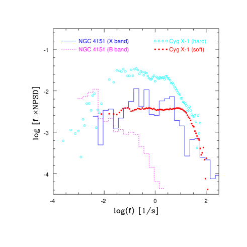
Figure 12: The NPSD for Cyg X-1 in the soft state, June 1996, (filled squares, from Gilfanov et al. 2000) and in the hard state February 3, 1997, (open circles), together with the NPSD for NGC 4151 in the optical band (dotted histogram) and in the X-ray band (continuous histogram), both shifted horizontally by 6.3 to account for a mass difference between the two sources.

The comparison of observational characteristics of galactic black hole candidates (GBH) and AGN is not straightforward. Observed photon spectra generally consist of two principal spectral components: soft bump usually interpreted as the accretion disk emission, and a power law interpreted as a result of Comptonization by a hot optically thin plasma. In AGN these components are well separated: the first one dominates the optical/UV emission, while the second one dominates the X-ray band. In galactic sources both are seen in X-ray band but their dominant role depends on the luminosity state of the source. Therefore, the power spectrum of a GBH in the hard, power-law dominated state should be compared with the X-ray power spectrum of an AGN while the power spectrum of a GBH in the soft disk-dominated state should be compared with the optical power spectrum of an AGN. While the former comparison has been attempted often in the past, the latter has not been addressed extensively.

X-ray power spectra of AGN are generally quite similar to power spectra of galactic objects in their hard state (see e.g. Czerny et al. 2001 and the references therein). The power peak in $f\times NPSD$ diagram is broad, covering about 2 decades, and its position on the frequency axis depends linearly on the mass of the black hole and can well be used for the mass determination (Hayashida et al. 1998; Czerny et al. 2001). A comparison of the X-ray power spectra of Cyg X-1 and NGC 4151 (Fig. 12) generally support this picture, and suggest that the mechanisms responsible for the emission and variability of the power law spectral component are indeed identical for AGN and GBH.

However, a comparison of the optical power spectrum of an AGN with power spectra of galactic sources in soft state does not show any striking similarity. In galactic sources the power is evenly distributed across the broad range of frequencies. In AGN, the longest timescales dominate. Our results for NGC 4151 confirm such a view (see Fig. 12). Timescales dominating the optical/UV variability in AGN (years) correspond to the timescales of hundreds/thousands of seconds in galactic sources. Strong outbursts with such timescales are only seen in the microquasar GRS1915+105 (see Belloni et al. 1997, Janiuk, Czerny, & Siemiginowska 2000). However, this source shows strong jet outflow and therefore it is not a simple analogue of a radio quiet Seyfert galaxy.

5.5 Decomposition of optical light curve into fast and slow variability components

The presence of the two separate types of variability - a slow component and a fast component - was already suggested by Belokon et al. (1978). Our results from the analysis of the PSD and SF in U and B bands based on much better data coverage confirm this result. Therefore, the data are not well represented by a sum of a constant component and a rapidly variable component, as suggested by Ulrich (2000).

In order to visualize the presence of the two separate types of variability – a slow component and a fast component– we complement the computations of the optical NPSD and the SF with a simple illustration. We calculate the smooth long timescale light curve at each data point by averaging all available data points separated from a given instance by less than adopted smoothing timescale, $\Delta T$. A representative set of such light curves for a range of $\Delta T$ is shown in Fig. 13.

Adopting $\Delta T=500$, we display the short timescale variations by subtracting the smoothed light curve from the original one (see Fig. 13, panel (a)). The result is shown in Fig. 13, panel (b). We see that the amplitude of variations display significant trends. This dependence of the amplitude on the flux was discussed by Doroshenko et al. (2001).

Such trends almost disappear if we plot the normalized light curve, i.e. if the value of the flux difference is divided by the value of the flux of the smoothed light curve (see Fig. 13, panel (c)). This figure provides an illustration of the same fact that was stressed by Uttley & McHardy (2001): only the normalized power spectrum is independent from the luminosity state of the source.

We can now compare these trends with variability of Cyg X-1 in its soft (disk-dominated) spectral state. In Fig. 13 (panel (d)) we show a sequence from the light curve of Cyg X-1 in February 3, 1997 (30 yr for NGC 4151 are equivalent to 300 s of Cyg X-1). We see that this light curve is clearly different from the original U-band light curve of NGC 4151 (see Fig. 2) but there is some similarity of Cyg X-1 light curve to that shown in panel (c) where all the long trends from NGC 4151 light curve have been removed. This supports our earlier conclusion that the fast optical variability component in AGN may well be connected with the X-ray reprocessing, and the X-ray variability itself is similar in AGN and GBH so the nature of fast variability might be the same in both types of objects.

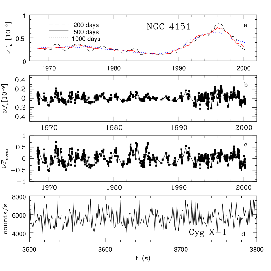
Figure 13: Panel (a): the smoothed light curve of NGC 4151 in U band, where smoothing timescales equal 200, 500 and 1000 days were used. Panel (b): the light curve of NGC 4151 in U band, with the long timescale trend of 500 days subtracted. Panel (c): the normalized light curve of NGC 4151 in U band, with the long timescale trend of 500 days subtracted. Panel (d): X-ray light curve of Cyg X-1 when the source was in the soft state (May 30, 1996). Errors in the Crimean data are $\sim 2.2$ %, errors in Cyg X-1 light curve are $\sim$ 25 cts s^-1.

5.6 Intrinsic variability versus obscuration

A number of authors suggested that the variable obscuration is, at least partially, responsible for the observed variability of AGN (e.g. Collin et al. 1996, Boller et al. 1997, Brandt et al. 1999, Abrassart & Czerny 2000, Risaliti, Elvis, & Nicastro 2002).

The absorbing column density in Ginga/EXOSAT data seems to be lower when the source is brighter (Yaqoob & Warwick 1991). However, if we look at the most recent and accurate observations, no obvious correlation is seen. In December 1993 when the AGN Watch monitoring was done the source was bright in U band ($\sim 75$ mJy; Kaspi et al. 1996, Crimean data) and the intrinsic X-ray column was $3.5\times 10^{22}$ cm^-2 (Edelson et al. 1996). In the beginning of March 2000 the source was faint in the U band ($\sim 21.5$ mJy; Crimean data) and the intrinsic X-ray column determined from the Chandra data was $3.7\times 10^{22}$ cm^-2 (Ogle et al. 2000).

On the other hand, the observed delays between the optical continuum and the emission lines (e.g. Kaspi et al. 1996) and between the optical emission and the infrared emission (e.g. Oknyanskij et al. 1999) show that the variability on the timescales of days is certainly intrinsic to the source, at least partially.

IUE monitoring during 18 years, which covered both the very low state around 1988 and the luminosity peak in the middle of outburst $\cal B$ around 1995 showed a factor over 12 increase in the flux although the UV line CIV1550 showed lower amplitude, by a factor of 5 (see Fig. 11 of Ulrich 2000). It might suggest that the continuum variations are additionally enhanced by some variations in the absorbing medium, perhaps due to variable ionization.

This shows that although the variable obscuration cannot be totally excluded, it cannot be the only factor responsible for the observed variability and most of variations are instead intrinsic to the source.

5.7 Interpretation of the variability

The strong variability of AGN in optical, UV and X-ray band is a well known but not well understood phenomenon (see Mushotzky, Done, & Pounds 1993; Ulrich, Maraschi, & Urry 1997). The observed properties of the X-ray time series indicate some stochastic process (McHardy & Czerny 1987; Czerny & Lehto 1997), which physically can be interpreted as magnetic flares above the cold disk or shocks developing in the hot accreting material. Optical variations are partially caused by reprocessing (although modeling is not simple; see e.g. Rokaki, Collin-Souffrin, & Magnan 1993; Kazanas & Nayakshin 2001; Życki & Różańska 2001; Wang, Wang, & Zhou 2001) and partially by another process operating on longer timescale, possibly the radiation pressure instability (e.g. Czerny et al. 1999).

The variability of the flux from the cold disk can be related to the Keplerian timescale, $t_{K}$, thermal timescale, $t_{th}$ or viscous timescale $t_{visc}$ of the accretion flow. The first value is universal (and depends only on the mass of the central object), and the other two can be computed for a Shakura-Sunyaev disk model. The variations due to the changes of properties of the hot plasma may also be related to $t_{K}$ and $t_{th}$, although the lack of theory for the dynamics of the hot phase makes this parameterization less firm.

To compute these time scales, we fix the mass of the black hole at $3.7\times 10^{7}M_{\odot}$, based on variability studies, and take the average luminosity to the Eddington luminosity ratio 0.02 resulting from the black hole mass value and the estimate of the total bolometric luminosity (see Czerny et al. 2001). For those parameters, we obtain the radial dependences of those timescales:

$$t_{K}=0.18m_{3.7}r_{10}^{3/2}~{}~{}~{}{\rm[d]},$$ (11)

$$t_{th}=1.8\alpha_{0.1}^{-1}m_{3.7}r_{10}^{3/2}~{}~{}~{}{\rm[d]},$$ (12)

$$t_{visc}=4000\alpha_{0.1}^{-1}m_{3.7}r_{10}^{7/2}\dot{m}_{0.02}^{-2}~{}~{}~{}{\rm[d]},$$ (13)

where $r$ is expressed in units of 10 Schwarzschild radii, $m$ in units of $3.7\times 10^{7}M_{\odot}$, and a standard viscosity parameter $\alpha$ in units of 0.1. The mass of the black hole enters the formulae linearly, and the accretion rate affects only the third quantity. In these computations we adopted $\dot{M}_{Edd}=1.69\times 10^{18}\times(M/M_{\odot})$ g s^-1, and $L_{Edd}=1.27\times 10^{38}\times(M/M_{\odot})$ erg s^-1, corresponding to the Newtonian accretion efficiency of 1/12.

We can now compare those timescales with the characteristic points present in the NPSD and SF both in the optical and in the X-ray band. The derived timescales are related to the Fourier frequencies: $f=(2\pi t)^{-1}$. The factor $2\pi$ is important if we want to compare the predicted timescales with the characteristic frequencies in the shape of the NPSD. Therefore, observed characteristic frequencies (1/5, 1/1000 and a lower limit of 1/4000 d^-1) translate into 0.8 d, 160 d, and more than 640 d, respectively. Here we used the timescales resulting from two-break fit (see Table 2), motivated by the analogy with the galactic sources.

The shortest X-ray timescale corresponds to the thermal timescale at the marginally stable orbit of the non-rotating black hole if the viscosity parameter is $\sim 0.03$, as obtained from spectral fits to the data for NGC 5548 (Kuraszkiewicz, Loska, & Czerny 1997). The value of the longest X-ray timescale is by a factor of 200 longer which suggests that the X-ray production region extends in that case up to $\sim 100R_{Schw}$, if timescale scaling as $r^{3/2}$ holds.

The timescale dominating the optical variability seems to be too long for pure thermal variations related to the radiation pressure instability. The thermal timescale of 640 d corresponds to a distance of $\sim 220$ $R_{Schw}$ (assuming $\alpha$ as above), much larger than the extension of the instability zone ($\sim 70$ $R_{Schw}$, calculated using the code of Róȧńska et al. 1999) for the adopted system parameters. Viscous timescales (see Eq. 13) on the other hand, are much longer than the period covered by the optical data. However, recent computations performed by Szuszkiewicz (1999) indicated much faster evolution than estimated from Eq. 13 - an outburst lasted $\sim 11$ years for adopted model parameters: $10^{8}M_{\odot}$ black hole, $\alpha=0.1$ and accretion rate $\dot{m}=0.06$.

Therefore, the observed variability in the optical band neither obviously proves nor contradicts the supposition that the optical variability at long timescales is caused by the radiation pressure instability of the optically thick disk. Further optical monitoring as well as theoretical progress are needed to resolve this issue. However, the lack of strong long timescale (hundreds of seconds) variability and the lack of radiation pressure dominated zone in Cyg X-1 (see e.g. Gierliński et al. 1999; Janiuk, Czerny, & Siemiginowska 2002), when compared with the presence of long timescale variations and the disk unstable zone in NGC 4151, favors the radiation pressure scenario. Analysis of the optical variability of NGC 5548 supported this view as well (Czerny et al. 1999).

6 Conclusions

Our analysis of the 90 years of the optical data and 27 years of the X-ray data for NGC 4151 using the NPSD and the SF techniques, gives the following results:

• variability properties in the optical and X-ray band are significantly different

• X-ray variations are predominantly in the frequency range 1/5 - 1/1000 $d^{-1}$

• optical variations are dominated by a component with a frequency on the order of (or possible smaller than) $\sim 1/5000$ d^-1 (or $\sim 10$ years), but the short timescale variability may be related to X-ray variability

• the presence of long timescale variability in NGC 4151 and the absence of analogous variability (on timescales of hundreds of seconds) in Cyg X-1 favors the radiation pressure mechanism

• the radial extension of the X-ray production region is similar in NGC 4151 and Cyg X-1 so the possible presence of radiation pressure dominated region in NGC 4151 and its absence in Cyg X-1 does not affect the X-ray production

Appendix A: Determination of the error on the power spectrum

Two methods can be used to estimate the errors on the power spectrum determined from observations. The first method is to assign directly the errors on the plotted histogram, and the second one is to do so through the Monte Carlo simulations. In this paper, we use both methods.

A.1 The direct method

The direct measurement error is estimated as follows. Discrete power spectrum computed at Fast Fourier Transform (FFT) frequency grid has a $\chi^{2}(2)$ distribution. Its variance matches the expected power. Whether the same is true for unevenly sampled data remains yet to be proven (e.g. Timmer & König 1995). Below, we adopt the same procedure, formal objections notwithstanding. Since we use logarithmic values (see Papadakis & Lawrence 1993), we estimate the error on the logarithmic value as follows. If the true value of the power is distributed around the measured value uniformly between 0 and twice the value, one sigma negative error would correspond to a value equal to 0.16 of the measured value. Therefore, the error of the logarithmic value on the negative side is equal to 0.43. We assume now that the errors are symmetric and adopt this value as a single measurement error of a single power spectrum in a single bin.

The power spectrum is computed in the frequency range determined by the data. It is subsequently binned into logarithmic bins of the width of 0.2. Measurements grupped into a single bin usually show significant dispersion, sometimes even higher than the single measurement error assigned above. Therefore we compute the error of a power spectrum in a bin by combining single measurement errors with the dispersion around the mean value $\bar{x}$

$$\sigma_{b}(f_{k})=({\sum_{i}{[x_{i}(f_{k})-\overline{x(f_{k})}]^{2}\over n_{k}^{2}}}+{0.43^{2}\over n_{k}^{2}})^{1/2}.$$ (14)

When separate sequences are computed overlapping in the frequency range we add the spectra in the common frequency bins assuming that the weight of the spectrum is inversely proportional to the measurement error of the contributing spectrum. The error of the resulting spectrum is again computed by combining the errors of the single measurements $\sigma_{b}^{i}$ (determined as described above) with the dispersion error

$$\sigma_{b}(f_{k})=({\sum_{i}{[x_{i}(f_{k})-\overline{x(f_{k})}]^{2}\over n_{k}^{2}}}+{\sum_{i}{(\sigma_{b}^{i})^{2}\over n_{k}^{2}})^{1/2}}.$$ (15)

This method is very simple and does not depend on the model of the power spectrum. However, it does not incorporate well the systematic errors caused by the window function.

A.2 Monte Carlo simulations of light curves

This method allows to estimate also the systematic effects of the window function as well as to draw the error contours for the adopted parameterization of the shape of the power spectrum.

In our approach we follow the method used by Uttley et al. (2002) and based on the method of Timmer & König (1995). It is equivalent to the method used by us in our previous paper (Czerny et al. 1999) which consisted of filtering the white noise with the filter corresponding to the adopted power spectrum distribution.

In our specific case we proceed as follows:

$\bullet$ We assume a shape of the NPSD in a form of either a broken power law with the slope 0 below the frequency break (parameters: frequency break and the slope above it) or in the form of a power law with two breaks and the slopes 0, 1 and 2 (parameters: two frequency breaks).

$\bullet$ We generate a random realization of this distribution by assuming the random uniform distribution of the power spectrum around the adopted value and the random distribution of Fourier phases. We generate an artificial equally spaced light curve that is somewhat longer than the duration of the data set through the FFT method. Next the light curve is folded with the observational window function thus reducing the long light curve to the number of points and spacing as in the observational data set.

$\bullet$ Next, we follow exactly the procedure applied to the observational data, i.e. we form yearly averages and other data subsets (see Sect. 3.1). We compute the power spectrum $NPSD_{i}(f)$ as we did for the observational data. We repeat the entire procedure $i=100-500$ times in order to create good statistics. The method is computationally intensive, so we cannot significantly increase this number for such a long and densely sampled data sets as used in our paper. From this distribution, we determine the average simulated power spectrum $\overline{NPSD(f)}$, and the dispersion $\sigma(\overline{NPSD(f)})$. We can assign a $\chi^{2}_{dist}(i)$ value to each of the simulated light curves: with the partial results forming the $\chi^{2}$ statistics around it

$$\chi^{2}_{dist}(i)=\sum_{k=1}^{kmax}{[NPSD^{i}(f_{k})-\overline{NPSD(f_{k})}]^{2}\over\sigma(\overline{NPSD(f_{k})})^{2}}.$$ (16)

The normalization of the power spectrum is adjusted to minimize the $\chi^{2}_{dist}(i)$ value.

$\bullet$ We also compute the same $\chi^{2}_{dist}(obs)$ value for the mean simulated power spectrum and the power spectrum determined from observations:

$$\chi^{2}_{dist}(obs)=\sum_{k=1}^{kmax}{[NPSD^{obs}(f_{k})-\overline{NPSD(f_{k})}]^{2}\over\sigma(\overline{NPSD(f_{k})})^{2}},$$ (17)

$\bullet$ The quality of the fit for a given power spectrum parameters is determined from the comparison of the value $\chi^{2}_{dist}(obs)$ with the distribution given by Eq. 16: the percentage of the light curves with the $\chi^{2}_{dist}(i)$ smaller than $\chi^{2}_{dist}(obs)$ gives the probability $P$ of the model rejection.

$\bullet$ Repeating the analysis for the range of the power spectrum parameters we find the best fit value (the highest acceptance probability) and we check if it is an acceptable model.

$\bullet$ Next, we determine the error contours for the two parameters of interest. For that purpose, we assume that the probability of any sets of values is proportional to the acceptance probability obtained above. We normalize the probability through performing the two-dimensional integral. We obtain the contour errors corresponding to the rejection probability of 68% ($\sim 1\sigma$ error) and 90% by integrating this renormalized probability over the surface through subsequent probability contours until the value of the integral is equal to 0.68 or 0.9, correspondingly. Since the computations were performed on a regular grid, in practice we find for example the contour level $P_{0.68}$ on the parameters of interest $x$ and $y$ iteratively from the expression

$$0.68={\sum_{i,k}^{if~{}P>P_{0.68}}P(x_{i},y_{k})\over\sum_{i,k}P(x_{i},y_{k})}.$$ (18)

Such contours are slightly smaller than contours plotted directly from the acceptance probability.

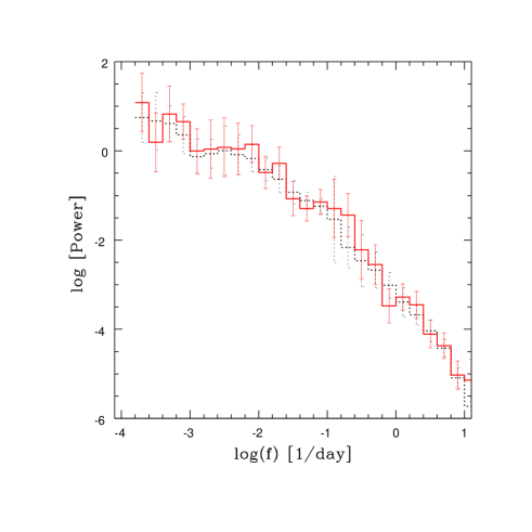
Figure 14: Observed NPSD in the X-ray band (continuous histogram) with errors determined directly from the data plotted against the best fit model (dotted histogram) of a single break power law with $\log f_{0}=-2.1$, $\alpha=1.5$. The $\chi^{2}_{dist}(obs)$ for this model is 13.39 for 22 dof (25 frequency points, 3 model parameters including normalization).

The comparison of the observed NPSD with the best fit model in X-ray band is shown in Fig. 14. The two distributions agree well within the indicated errors.

6.0.1 Comparison with standard $chi^{2}$ statistics

We also performed an exercise of applying the theory lying behind the proper $\chi^{2}$ distribution. We used the best fit value of $\chi^{2}_{dist}(obs)$ from the Table 2 and determined the error contour by adding the standard value of 4.61 (Avni 1976) for 90% error, two parameters of interest (see Fig. 15). Such a contour is much more compact than the contour determined directly from the simulations, as described above. This is surprising since the histogram of $\chi^{2}_{dist}(i)$ approximates quite well the theoretical $\chi^{2}$ histogram (see Fig. 16) for the appropriate number of degrees of freedom (22 in the case of X-ray data). Error contours determined from simulations correspond to adding a value of order of $\sim 8-28$ to the best fit $\chi^{2}_{dist}(obs)$. This shows that the Monte Carlo simulations are indeed extremely important, as argued by Uttley et al. (2002).

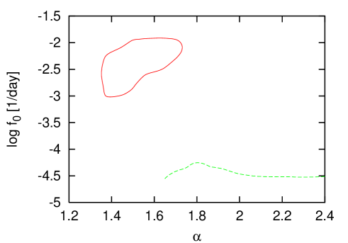
Figure 15: Error contour at 90% confidence level for the broken power law model of X-ray and optical NPSD determined as $\chi^{2}_{min}+4.61$; to be compared with thin lines in Fig. 4, upper panel.

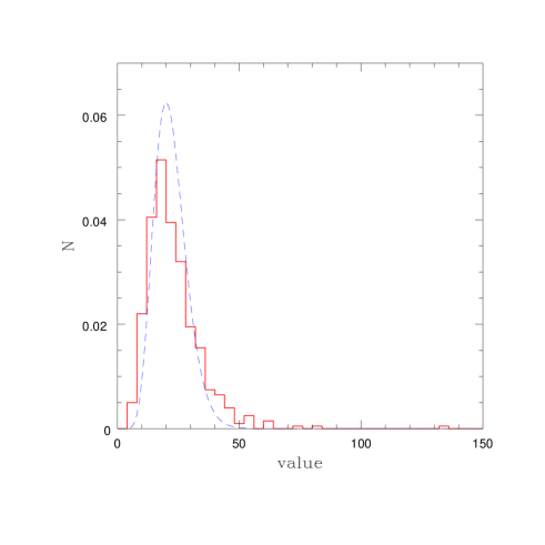
Figure 16: The distribution of the $\chi^{2}_{dist}(i)$ values (histogram) for 500 Monte Carlo curves in comparison with the $\chi^{2}$ theoretical plot for 22 dof. Parameters: X-ray data, model of a single break power law with the best fit parameters: $\log f_{0}=-2.1$, $\alpha=1.5$.

Appendix B: Structure function - error determination

We again use two methods in order to determine the errors. The first method is to assign directly the error of the structure function obtained observationally. The second method includes the Monte Carlo simulations. Both methods are used in the present paper.

B.1 The direct method

The structure function is computed in the timescale range determined by the data. We use logarithmic time bins with a width of 0.16. We determine the SF for bins with the number of pairs available greater than 7 pairs. The errors are assumed to come both from the flux measurement error and from the limited statistics of pairs. The flux measurement error is small, particularly for the photoelectric optical data (0.01, 0.015 and 0.02 - 0.025 mag for V, B and U band, correspondingly). The error on the data determined from the old photographic plates is below 20% and the X-ray data have errors of order of 10%. Therefore, statistical errors dominate.

The statistical uncertainty in the SF$(\tau_{k})$ is equal to the ratio of the dispersion in the SF at a given bin to the number of pairs, i.e.

$$\sigma^{2\quad(st)}_{SF}(\tau_{k})=\sum_{ij}\frac{(x_{i}-x_{j}-(\overline{x_{i}-x_{j}}))^{2}}{(n_{k}/2)^{2}}\ ,$$ (19)

where $\overline{x_{i}-x_{j}}$ is the mean pair difference and $n_{k}$ is the number of pairs in bin k. This error is plotted in Fig. 6.

In our error analysis we included two additional effects, which should render the error determination more robust.

For completeness, we took into account the errors associated with the flux measurements. This can be easy assessed through Monte Carlo simulations. Assuming that the errors in fluxes are normally distributed, we can modify each flux by random Gaussian deviates based on the quoted error for each data point. In a single Monte Carlo realization each data point is modified, and the SF is computed. Computing a large number of independent realizations (500 - 1000) we obtain the mean SF and the rms deviation of the mean SF. We call this rms deviation to result from flux randomization $\sigma^{2\quad(fr)}_{SF}(\tau_{k})$ (see Peterson, Wanders and Horne 1998). The third source of errors is associated with the observational sampling of the light curves. The specific times of observations are in a sense ’randomly distributed’ and the SF can be less sensitive to the choice of individual data points than the power spectrum. We can estimate these uncertainties through considering subsets of the original “parent” data set. This method is known as the bootstrap method. It can be used to evaluate the significance of the SF itself, its rms and other parameters such as slope ”b” of SF. The method works as follows:

We have a set of observations (t1,x1), (t2,x2),…, (tn,xn). We can take from this set n pairs of randomly selected points without regard to whether or not they have been previously selected. Thus we select a subset of the original data points, in which some data pairs repeat more than once and some of the original pairs are ignored. Next the multiple pairs are removed so the size of the selected sample is reduced. For this data set we again calculate the SF and we repeat this process many times (500 - 1000). Multiple realizations lead to a mean and standard deviation for the structure function based on a randomly chosen subset of the original data points. We mark this rms value describing the effect of random subset selection as $\sigma^{2\quad rss}_{SF}(\tau_{k})$.

Our computations show that bootstrapping gives the most conservative values of uncertainties in comparison with the other two described above. This is probably due to the fact that the considered subsets have smaller number of points than the real light curve.

The total uncertainty of the SF can be obtained if we assume that the errors add in quadrature.

$$\sigma^{2}_{SF}(\tau_{k})=\sigma^{2\quad(st)}_{SF}(\tau_{k})+\sigma^{2\quad fr}_{SF}(\tau_{k})+\sigma^{2\quad rss}_{SF}(\tau_{k})\ .$$ (20)

These error bars are used in Figs. 8 and  9. This procedure allows us also to estimate the best-fit value and uncertainties of such parameter as a slope $b$ of linear part of the SF.

We note here that all those uncertainties are model independent.

B.2 Monte Carlo simulations of light curves

In order to estimate the errors of the SF without a significant loss of information appearing in the bootstrap method we also perform the Monte Carlo simulations of the light curve itself based on the specific SF model.

The SF with the linear part having the slope $b$ can be obtained within the frame of the Poissonian model also called “shot noise” model. It means that in a physical system the variations are due to the stochastic superposition of independent flares of a given basic shape randomly distributed in time, but of various durations and amplitudes. Under certain conditions, imposed on the flare, the amplitudes and durations of such process may result in the first-order structure function $SF(\tau)$ being a power law of $\tau$ with an index $b$ which takes on values from 0 to 2 (e.g. Terebizh et al. 1989; Sergeev 1999, Cid Fernandes, Sodr’e, & Vieira da Silva 2000).

Sergeev (1999) showed that if the number $n$ of flares of duration $T_{f}$ is given by a power law distribution, i.e.

$$n(T_{f})\sim T_{f}^{\alpha}$$ (21)

and if the flare amplitude $A(T_{f})$ also depends on the flare duration as a power law,

$$A(T_{f})\sim T_{f}^{\beta},$$ (22)

then the dependence of the structure function on the interval $\tau$ asymptotically converges to a power law shape

$$SF(\tau)\sim\tau^{b},~{}~{}~{}~{}~{}b=\alpha+2\beta+2.$$ (23)

In the considerations of Sergeev (1999), the extension of the power law dependencies of the flare parameters given by Equations 21 and 22 were limited by a natural physical constraints: the flare duration was allowed to vary only between $T_{f}^{min}$ and $T_{f}^{max}$. The adopted shape of the flares was Gaussian, but it was shown that the profiles of flares are of no importance. Flares can have any profile: square, triangle or Gaussian (e.g. Sergeev 1999, Cid Fernandes et al. 2000).

We performed Monte Carlo simulations using the software of Sergeev with 5 input free parameters:

1. dT(flare)= the mean time interval between two flares

2. $\alpha$ = index in the dependence of flare numbers on duration,

3. $\beta$ = index in the dependence of the flare amplitude on duration,

4. $T_{min}$ = minimal duration of flares

5. $T_{max}$ = maximal duration of flares.

Using Sergeev’s program for simulation of light curves, we modeled such light curves using various values of $\alpha$ and $\beta$. It is important to stress, however, that it is impossible to obtain separately the values of the parameters $\alpha$ and $\beta$. Therefore, we took into account the relation $b=2+\alpha+2\beta$, where $b$ is a slope of the SF determined from observations.

Changing all 5 parameters we simulated a number of light curves (N$\sim$500 - 1000) in each energy band and we computed the SF for each simulated light curve in the same manner as we did for the observed light curve. From each bin of all calculated SFs we subtracted $2D_{err}$ with $D_{err}$ being the mean variance of the measurement uncertainties. The model SF (corresponding to the given model and sampling pattern of the observed light curve) is then given by the mean of the N simulated SFs, $\overline{SF(\tau)_{sim}}$. The model error is given by the rms spread of the simulated model population around the mean value at each time interval $\tau$, $\sigma(\tau)_{sim}$.

The quality of the model representation of the observational light curves is estimated with help of statistics $\chi^{2}_{test}$, which we calculate as follows:

$$\chi^{2}_{test}=\sum_{T_{f}=T_{min}}^{T_{f}=T_{max}}\frac{[\overline{SF(\tau)_{sim}}-SF(\tau)_{obs}]^{2}}{\sigma^{2}(\tau)_{sim}}$$ (24)

We assumed that the best parameters of model are those yielding the minimum value of $\chi^{2}_{test}$ and the values of these parameters are listed in Table 4.

This paper has been processed by the authors using the Blackwell Scientific Publications LaTeX  style file.

References

- [] Abrassart A., Czerny B., 2000, A& A, 356, 475
- [] Avni Y., 1976, ApJ, 210, 642
- [] Belloni T., Mendez M., King A.R., van der Klis M., van Paradijs J., 1997, ApJ, 479, L145
- [] Belokon E.T., Babadzanjantz M.K., Lyutyi V.M., 1978, A&ASS, 31, 383
- [] Boller Th., Brandt W.N., Fabian A.C., Fink H.H., 1997, MNRAS, 289, 393
- [] Borczyk W., Schwarzenberg-Czerny A., Szkody, P., 2003, A&A (submitted)
- [] Brandt J.C., et al., 2001, AJ, 121, 2999
- [] Brandt W.N., Boller Th., Fabian A.C., Ruszkowski M., 1999, MNRAS, 303, L53
- [] Cannon R.D., Penston M.V., Brett R.A., 1971, MNRAS, 152, 79
- [] Cid Fernandes, R., Sodr’e Jr, L., Vieira da Silva, L., 2000, ApJ, 544, 123
- [] Collin-Souffrin S., Czerny B., Dumont A.-M., Życki P.T., 1996, A&A, 314, 393
- [] Collier S., Peterson B.M., 2001, ApJ, 555, 775.
- [] Czerny B., Lehto J.H., 1997, MNRAS, 285, 365
- [] Czerny B., Nikołajuk M., Piasecki M., Kuraszkiewicz J., 2001, MNRAS, 325, 865
- [] Czerny B., Schwarzenberg-Czerny A., Loska Z., 1999, MNRAS, 303, 148
- [] Doroshenko V.T., et al. 2001, AstL, 27, 65
- [] Edelson R. et al. 1996, ApJ, 470, 364
- [] Evans I. N., Tsvetanov Z., Kriss G. A., Ford H. C., Caganoff S., Koratkar A. P., 1993, ApJ, 417, 82
- [] Fan J.-H., Su C.-Y., 1999, ChA&A, 23, 22
- [] Fiore F., Massaro E., Perola G.C., Piro L., 1989, ApJ, 347, 171
- [] Fitch W.S., Pacholczyk A.G., Weymann R.J., 1967, ApJ, 150, 67
- [] Gierliński M., Zdziarski A., Poutanen J., Coppi P.S., Ebisawa K., Johnson W.N., 1999, MNRAS, 309, 496
- [] Gilfanov M., Churazov E., Revnivtsev M., 2000, MNRAS, 316, 923
- [] Hayashida K., Miyamoto S., Kitamoto S., Negoro H., Inoue H., 1998, ApJ, 500, 642
- [] Janiuk A., Czerny B., Siemiginowska A., 2000, ApJ, 542, L33
- [] Janiuk A., Czerny B., Siemiginowska A. 2002, ApJ, 576, 908
- [] Johnson W.N., McNaron-Brown K., Kurfess J. D., Zdziarski A. A., Magdziarz P., Gehrels N., 1997, ApJ, 482, 173
- [] Kaspi S., et al. , 1996, ApJ, 470, 336
- [] Kataoka J., et al., 2001, ApJ, 560, 659
- [] Kazanas D., Nayakshin S., 2001, ApJ, 550, 655
- [] Kolmogorov A.N., 1941a, Dokl.Acad.Nauk.SSSR, v.30, p.229
- [] Kolmogorov A.N., 1941b, Dokl.Acad.Nauk.SSSR, v.32, p.19
- [] Kriss G.A., Davidsen, A.F., Blair, W.P., Bowers, C.W. Dixon, W.V. et al. 1992, ApJ, 392, 485
- [] Kuraszkiewicz J., Loska Z., Czerny B., 1997, Acta Astr., 47, 263
- [] Leighly K., 1999, ApJSS, 125, 297
- [] Longo G., Vio R., Paura P., Provenzale A., Rifato A., 1996, A& A, 312, 424
- [] Lyuty V.M., Doroshenko V.T., 1999, Astron. Lett., 25, 341
- [] Lyutyj V.M., Oknyanskij V.L., Chuvaev K.K. 1984, Sov. Astron. Let., 10, 335
- [] Lyutyj V.M., Oknyanskij, V.L. 1987 Astron.Zhurnal, 64, 465
- [] Lyutyi V.M.,Taranova, O.G., Shenavrin, V.I. 1998 Astron. Lett., 24, 199
- [] Manners J., Almaini O., Lawrence A., 2001, MNRAS, 330, 390
- [] Markowitz, A., Edelson, R., 2001, ApJ, 547, 684
- [] McHardy I.M., Czerny B., 1987, Nat., 325, 696
- [] Merkulova N.I., Metik L.P., Pronik I.I., 2001, A&A, 374, 770
- [] Mushotzky R.F., Done C., Pounds K.A., 1993, ARA&A, 31, 717
- [] Ogle P.M., Marshall H.L., Lee J.C., Canizares C. R., 2000, ApJ, 545, L81
- [] Oknyanskiy V.L., 1978, Perem. Zvezdy, 21, 71
- [] Oknyanskiy V.L., 1983, Astron.Circuliar, 1300, 1
- [] Oknyanskij V.L., 1994, Astrophysics and Space Science, 222, 157
- [] Oknyanskij V.L., Lyuty V.M., Taranova O.G., Shenavrin V.I., 1999, Astronomy Letters, 25, 483
- [] Pacholczyk A.G., 1971, ApJ, 163, 449
- [] Pacholczyk A.G., et al., 1983, Astroph. Letters, 1983, 23, 225
- [] Paltani S., Courvoisier T.J.-P., Walter R., 1998, A&A, 340, 47
- [] Papadakis I., McHardy I.M., 1995, MNRAS, 273, 923
- [] Papadakis I., Lawrence A., 1993, MNRAS, 261, 612
- [] Penston M.V., Pérez E. 1984, MNRAS, 211, 84
- [] Penston M.V., Penston, M. J., Neugebauer G., Tritton K. P., Becklin, E. E., Visvanathan, N., 1971, MNRAS, 153, 29
- [] Perez G. et al. 1998, ApJ, 500, 685
- [] Perotti F. et al., 1990, ApJ, 356, 467
- [] Peterson B.M., Wandel A., 1999, ApJ, 521, L95
- [] Peterson B.M., Wanders I., Horne K., 1998, PASP, 110, 660
- [] Pottschmidt K., et al., 2002, A& A (astro-ph/0202258)
- [] Press W.H., Rybicki G.B. 1997, in Astronomical Time Series, ed. D. Maoz, A. Sternberg, & E. M. Leibowitz Dordrecht, Kluwer, p. 61
- [] Pronik S. G., Sergeev V.I., Sergeeva E. A., 2001, ApJ, 554, 245
- [] Reina C., Tarenghi M., 1973, A&A, 26, 257
- [] Risaliti G., Elvis M., Nicastro F., 2002, ApJ, 571, 234
- [] Rokaki E., Collin-Souffrin S., Magnan C., 1993, A&A, 272, 8
- [] Różańska A., Czerny B., Życki P.T., Pojmański G., 1999, MNRAS, 305, 481
- [] Sergeev S.G., 1999, Candidate’s dissertation, Krymsk. Astrofiz. Obs., Crimea
- [] Sergeev S.G., Pronik V.I., Sergeeva E.A., Malkov Yu.F., 1999,ApJSS, 121, 159
- [] Shakura N.I., Sunyaev R.A., 1973, A&A, 24, 337
- [] Siemiginowska A., Czerny B., 1989, MNRAS, 239, 289
- [] Simonetti J.H., Cordes J.M., Heeschen D.S., 1985, ApJ 1985, 296, 46
- [] Szuszkiewicz, E., 1999, Mem.S.A.It, 70, 95
- [] Terebizh V.Yu., Terebizh A.V. & Biryukov V.V., 1989, Astrofizika, 31, 75
- [] Timmer J., König M., 1995, A&A, 300, 707
- [] Ulrich M.-H., 2000, A&ARv, 10, 135
- [] Ulrich M.-H., Maraschi L., Urry M.C., 1997, ARA&A, 35, 445
- [] Uttley P., McHardy I.M., 2001, MNRAS, 323, L26
- [] Uttley P., McHardy I.M., Papadakis I.E., 2002, MNRAS, 332, 231
- [] Wandel A., Peterson B.M., Malkan M.A., 1999, ApJ, 526, 579
- [] Wang J.-X., Wang T.-G., Zhou Y.-Y., 2001, ApJ, 549, 891
- [] Ward M.J., Geballe T., Smith M., Wade R., Williams P., 1987, ApJ, 316, 138
- [] Weaver K.A., Yaqoob T., Holt S.S., Mushotzky R.F., Matsuoka M., Yamauchi M., 1994, ApJ, 436, L27
- [] Wu Ch.-Ch., Weedman D.W. 1978, ApJ, 223, 798
- [] Yaqoob T., et al, 1993, MNRAS, 262, 435
- [] Yaqoob T., Warwick R.S., 1991, MNRAS, 248, 773
- [] Zdziarski A.A., Johnson W.N., Magdziarz P., 1996, MNRAS, 283, 193
- [] Życki P.T., Różańska A., 2001, MNRAS, 325, 197